Article

Pipeline Corrosion Prediction Using the Grey Model and Artificial Bee Colony Algorithm

School of Mechanical Engineering and Automation, University of Science and Technology Liaoning, Anshan 114051, China
*
Author to whom correspondence should be addressed.
Axioms 2022, 11(6), 289; https://doi.org/10.3390/axioms11060289
Submission received: 1 May 2022 / Revised: 6 June 2022 / Accepted: 8 June 2022 / Published: 14 June 2022
(This article belongs to the Special Issue Differential Equations and Genetic Algorithms)

Abstract

:
Pipeline corrosion prediction (PCP) is an important technology for pipeline maintenance and management. How to accurately predict pipeline corrosion is a challenging task. To address the drawback of the poor prediction accuracy of the grey model (GM(1,1)), this paper proposes a method named ETGM(1,1)-RABC. The proposed method consists of two parts. First, the exponentially transformed grey model (ETGM(1,1)) is an improvement of the GM(1,1), in which exponential transformation (ET) is used to preprocess the raw data. Next, dynamic coefficients, instead of background fixed coefficients, are optimized by the reformative artificial bee colony (RABC) algorithm, which is a variation of the artificial bee colony (ABC) algorithm. Experiments are performed on actual pipe corrosion data, and four different methods are included in the comparative study, including GM(1,1), ETGM(1,1), and three ETGM(1,1)-ABC variants. The results show that the proposed method proves to be superior for the PCP in terms of Taylor diagram and absolute error.

1. Introduction

The pipeline is highly susceptible to leakage owing to the corrosive medium it conveys [1]. Pipeline corrosion prediction (PCP) technology, therefore, becomes the focus of pipeline protection efforts and is a prerequisite for determining pipeline maintenance cycles and measures.
A lot of work has been done on the PCP. At present, the main methods of the PCP are neural networks [2], grey models (GM(1,1)) [3], and hybrid models. Neural networks are utilized for the PCP. Pedapati et al. [4] used neural networks to develop an intelligent model that predicted results closer to the true value. Wen et al. [5] proposed a modeling approach using neural networks to assess the corrosion condition of natural gas pipelines. The results showed that the proposed model could reliably predict the corrosion trend of natural gas pipelines. Shaik et al. [6] established the relationship between corrosion factors and the corrosion status of a pipeline through neural networks in the case of a large number of data samples, which could accurately predict the life of a pipeline. The grey model (GM(1,1)) is another method to predict pipeline corrosion. In practical application, the model prediction accuracy is often not high owing to its own shortcomings. For this reason, researchers have continuously proposed various improvement approaches. Liao et al. [7] proposed the optimized grey model (OGM(1,1)) that could effectively estimate the corrosion rate of pipelines with multiple factors considered. Gao et al. [8] developed an improved grey model (IGM(1,1)) to predict submarine pipeline corrosion. Zheng et al. [9] developed a GM-RBF neural network corrosion rate prediction model based on the error compensation principle to accurately predict the remaining life of subsea oil and gas pipelines subject to corrosion. Deng et al. [10] combined grey correlation analysis and fuzzy neural network as a new corrosion prediction method, which had high prediction accuracy and application value. Jiang et al. [11] combined the GM(1,1) and BP neural network to build G-B-I and G-B-II prediction models, which had significantly lower prediction errors as well as superior predictive power. Hybrid models are also widely used in the PCP. Peng et al. [12] proposed a hybrid intelligent method to predict the corrosion rate of multiphase flow pipelines, and the results showed that the method had good performance in the prediction of the corrosion rate of multiphase flow pipelines. Li et al. [13] proposed a new data-driven model based on hybrid techniques to simulate corrosion degradation in subsea operations. The model enabled the effective prediction of corrosion rates. Peng et al. [14] presented a comprehensive review of pipeline corrosion assessment from the perspective of data analysis and proposed a corrosion growth model aimed at predicting future corrosion states to achieve effective prediction of corrosion rates. Abyani et al. [15] proposed a new method for assessing the reliability of pipeline corrosion using finite element simulation, which achieves an effective prediction of corrosion rates. Deif et al. [16] uses passive RFID sensors to collect field data and then integrates them into a building information modeling (BIM) system to enable effective prediction of corrosion rates.
GM(1,1) is widely used because it does not require a large number of samples and has a low computational effort. However, GM(1,1) has its own drawbacks, such as unsmoothed original series and large prediction errors generated by the construction of background values. To overcome these drawbacks, this paper introduces exponential transformation and dynamic coefficients into the GM(1,1) to preprocess the raw data and reconstruct the background values, respectively. Then artificial bee colony (ABC) algorithm is used to optimize the dynamic coefficients to improve the prediction accuracy. The artificial bee colony (ABC) algorithm is one of the swarm intelligence (SI) algorithms [17]. SI algorithms have been used in real-world applications to solve complex problems [18]. A wide variety of the optimization algorithms have been proposed to solve the parameter optimization problem, such as particle swarm optimization (PSO) [19], genetic algorithm (GA) [20], differential evolution (DE) algorithm [21], bacterial foraging optimization (BFO) algorithm [22], and ant colony algorithm (ACO) [23]. The specific objective of this study was to use a new method for the PCP. The contributions of this paper are as follows:
(1)
Exponentially transformed and dynamic coefficients are added to the traditional GM(1,1).
(2)
An improved version of the ABC algorithm, called the reformative artificial bee colony (RABC) algorithm, is proposed and its performance is verified by benchmark functions.
(3)
The exponentially transformed grey model (ETGM(1,1)) combined with RABC, called ETGM(1,1)-RABC, is proposed for the PCP.
(4)
The superiority of ETGM(1,1)-RABC is verified through experiments.

2. Related Theory

This section introduces the related theory for the PCP, including the GM(1,1) and ABC algorithm.

2.1. GM(1,1)

The GM(1,1) uses the accumulation of the original sequences to generate new sequences so that the raw chaotic data show regularity and good prediction results can be obtained even with only a relatively small amount of data. The GM(1,1) consists of three steps: cumulative generation, modeling solution, and cumulative reduction, which are described in detail as follows [24]. The flowchart of the GM(1,1) is shown in Figure 1.
(1)
Cumulative generation. Let X(0) = (x(0) (1), x(0) (2),…, x(0) (n)) be the original non-negative sequence; then let X(1) = (x(1) (1), x(1) (2),…, x(1) (n)) be the first-order cumulative sequence of X(0); here, x(1) (k) can be expressed as
x 1 ( k )   =   i   =   1 k x 0 i
where k = 1, 2,…, n, and n is the raw data length.
Let Z(1) = (z(1) (2), z(1) (3),…, z(1) (n)) be the immediate mean sequence X(1); here, z(1) (k) can be expressed as
z 1 k   =   1 2 x 1 k   +   x 1 k     1
(2)
Modeling solution. Let x(0) (k) + az (1) (k) = b be the grey differential equation for the GM(1,1), then the whitening differential equation can be expressed as
d x 1 t d t   +   a x 1 t   =   b
where a is the development factor; b is the amount of grey action; a and b are both parameters to be solved; and the values of a and b can be estimated by the least-squares method, which can be expressed as follows
a , b T   =   B T B     1 B T Y
where
B   =   z 1 2 1 z 1 3 1 z 1 n 1 Y   =   x 0 2 x 0 3 x 0 n
Then, the solution for the whitening differential equation is expressed as follows
x 1 t   =   b a   +   x 1 1     b a e a t     1
The cumulative predicted values are then obtained as follows
x ^ ( 1 ) k   +   1   =   b a   +   x 0 1     b a e a k
where k = 1, 2,…, n − 1.
(3)
Accumulation reduction. Thus, the corresponding predicted values are obtained as follows
x ^ ( 0 ) k   +   1   =   x ^ ( 1 ) k   +   1     x ^ ( 1 ) k

2.2. Basic ABC Algorithm

The basic ABC algorithm is divided into four stages: initial stage, employed bee phase, onlooker bee phase, and scout bee stage [25].
In the initial stage, The ABC algorithm generates the initial population using the following equation.
X i j   =   X min j   +   r a n d ( 0 , 1 ) ( X max j     X min j )
where i = 1,…, SN, j = 1,…, D. SN denotes the population size, D denotes the dimension of the problem, and rand(0, 1) is a random number between 0 and 1. X max j and X min j denotes the upper and lower bounds of the jth dimension of the individual, respectively. The fitness function of a solution can be expressed as
f i t i   =   1 1   +   f ( X i ) f ( X i ) 0 1   +   f ( X i ) f ( X i ) < 0
where f (Xi) is the objective function value of the ith food source.
In the employed bee phase, the employed bees use Equation (10) to perform a random search of the neighborhood to find the food source and pass the food source information to the onlooker bee waiting in the hive.
V i j   =   X i j   +   φ i j X i j     X k j
where k ∈ (1,…, SN) and kI, where k is chosen randomly, which means that there is only one randomly chosen solution in generating the new candidate solution; j ∈ (1,…, D), where j is also chosen randomly, which means that only one dimension has changed between the new candidate solution and the old one. φ i j is a random number uniformly distributed on [–1, 1].
In the onlooker bee phase, based on the food source information passed back to the hive by the employed bees, the onlooker bees use roulette to select the food source according to the probability calculated in Equation (11) below, and the food source is still updated randomly using Equation (10).
P i   =   f i t i Σ i   =   1 S N f i t i
where fiti is the fitness value of the ith food source.
In the scout bee stage, a food source whose quality has not been getting better will be discarded. The onlooker bee searching for this food source will turn into the scout bee. In the ABC algorithm, the food source corresponds to the candidate solution of the optimization problem, and the quality of the food source represents the good or bad candidate solution.

3. Proposed Method

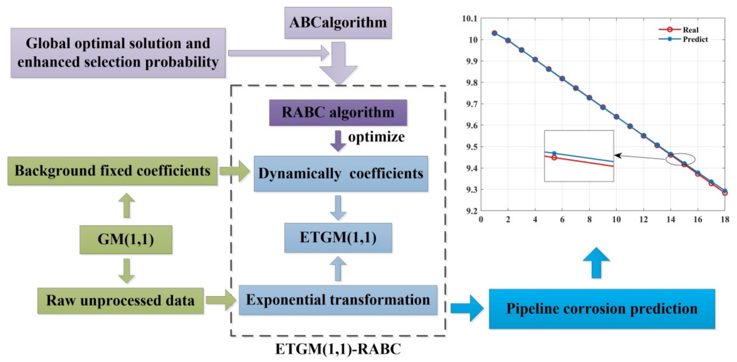
The ETGM(1,1) in this paper is an improvement of the GM(1,1). There are two improvements to the GM(1,1); one is to change the background fixed coefficients of the grey model into dynamic coefficients, and the other is to preprocess the original data using exponential transformation. The dynamic coefficients are optimized by an RABC algorithm that introduces a global optimal solution and enhancement for selection probability. The schematic of the proposed method is portrayed in Figure 2.

3.1. Exponential Transformation (ET) for the Raw Data

The prediction accuracy of the GM(1,1) will be greatly reduced when dealing with the raw data with insufficient smoothness. A common method is to preprocess the raw data using a data transformation to improve its smoothness [26]. In this paper, the ET is used to preprocess the raw data, and the specific process is as follows.
An ET of the raw data can be expressed as
y 0 i   =   c x 0 k , i   =   k   =   1 , 2 , , n
where c is the base number. The modeling solution for the above exponentially transformed data is to obtain the new cumulative predicted values that are expressed as follows
y ^ 1 k   +   1   =   b a   +   y 0 1     b a e a k
The predicted values of the new cumulative predicted values are expressed as
y ^ 0 k   +   1   =   y ^ 1 k   +   1     y ^ 1 k
Because y(0) (k) = cx(0) (k), the predicted value of the raw data can be given by
x ^ 0 k   =   ln y ^ 0 k ln c

3.2. Introducing Dynamic Coefficients

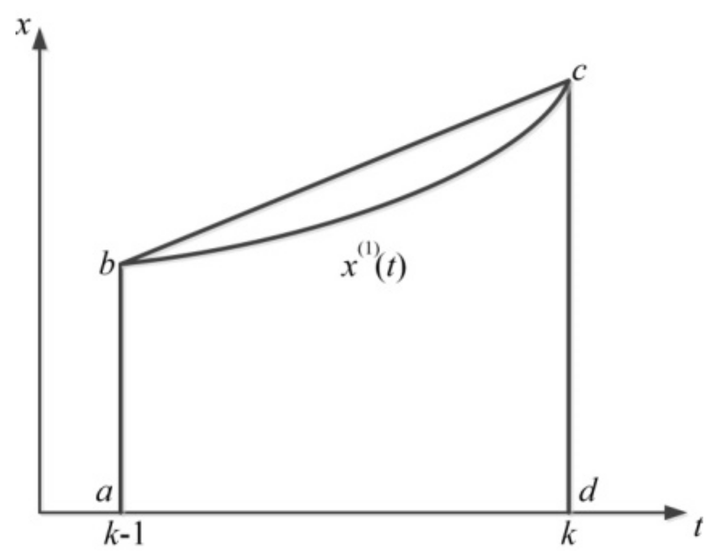
GM(1,1) is flawed in constructing the background values. The true background value should be the integral of x(1) (t) over the interval [k − 1, k], whereas the background value obtained by GM(1,1) is the trapezoidal area, as shown in Figure 3. If the raw data changes more drastically, the background value construction of the GM(1,1) will bring large errors and lead to a decrease in prediction accuracy [27]. This paper uses dynamic coefficients α (i) instead of fixed coefficients to minimize the background value error by dynamically adjusting the coefficients for each interval. The new equation for constructing the background values is as follows
z ^ 1 k   =   α i x 1 k   +   1     α i x 1 k     1
where α (i) is the dynamic coefficient, 0 ≤ α (i) ≤ 1, i = 1, 2,…, n − 1, k = 2, 3,…, n.
The ABC algorithm is used to solve the dynamic coefficients because the ABC algorithm has a unique advantage in solving non-linear, multi-dimensional complex optimization problems. In the next section, the RABC algorithm will be presented and its performance will be verified by benchmark functions.

3.3. RABC Algorithm

This is example 1 of an equation. The RABC algorithm is an upgraded version of the ABC algorithm. One of the upgrades is the search equation for the food source. The search equation in the RABC algorithm is added to the global optimal food source so that the bees search around better quality food sources. Using the optimal food source as a reference improves the searchability of the algorithm to some extent. The search equation in the RABC algorithm can be given by
V i j   =   X i , b e s t j   +   φ i j X i , b e s t j     X i j
where X i , b e s t j is the globally optimal food source.
The selection probability of bees is determined by the proportion of fitness of the current food source among all food sources. Less difference between the better food source and the optimal food source leads to a lower probability of selection of the optimal food source. The chance to search for some bad food source results in slowing down the speed of finding the optimal food source owing to the random selectivity in the ABC algorithm. In this paper, we propose to use the current optimal fitness as a reference to improve the speed of the colony in finding the optimal food source. Thus, the selection probability can be given by
P i   =   0.8 f i t i f i t max   +   0.2
where fitmax is the fitness value for the optimal solution.
Using Equation (17) to update the food source location ensures that the bees are not disturbed by the locally optimal bees, but also that the bees move to a better food source led by the globally optimal bees. Equation (18) enhances the probability of exploitation of high-quality food sources.

3.4. Verification for RABC Algorithm

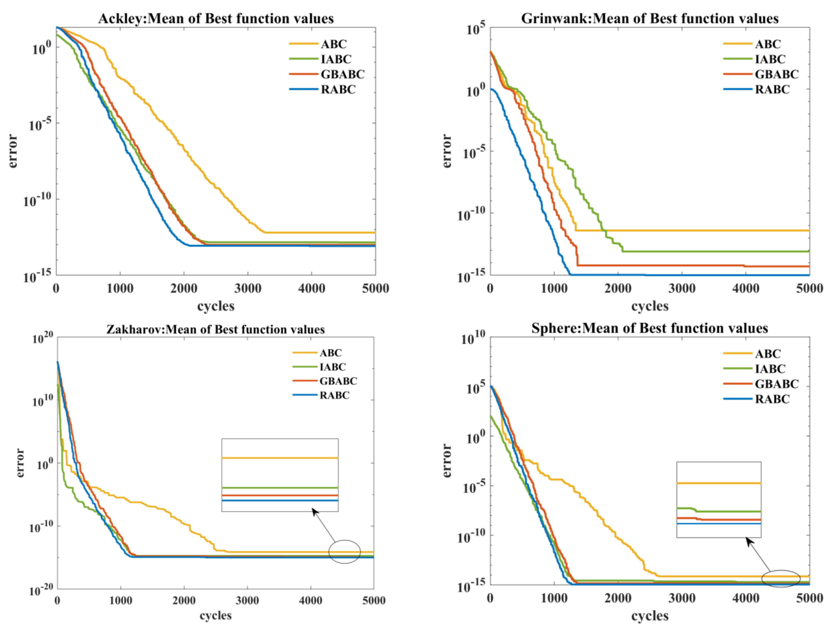
To verify the performance of the RABC algorithm, the ABC algorithm, IABC algorithm [28], and the GBABC algorithm [29] are used as a comparison based on four benchmark functions. The benchmark functions are given in Table 1. The parameters of the three algorithms are set as follows: D = 50, SN = 100, limit = 50, and Maxcycle = 5000, and each algorithm is run independently 30 times. The results are shown in Table 2 and Figure 3. The parameters in each algorithm are set to be the same or optimal for fairness.
Table 2 shows the results of the ABC, BC, GBABC, and RABC algorithms for four benchmark functions. From Table 2, we can see that, except for the std value of F4, the mean and std values of the IABC algorithm are smaller than those of the ABC algorithm. It is worth noting that the RABC algorithm has a better mean and std than the ABC, IABC, and GBABC algorithms for the four benchmark functions. Figure 4 shows the convergence obtained by the four algorithms. From Figure 4, the convergence speed of the RABC, IABC, and GBABC algorithms is superior to that of the ABC algorithm. Further, the convergence speed of the RABC algorithm is slightly better than that of the IABC and GBABC algorithms. The above results indicate that some improvements enhance the ABC algorithm.
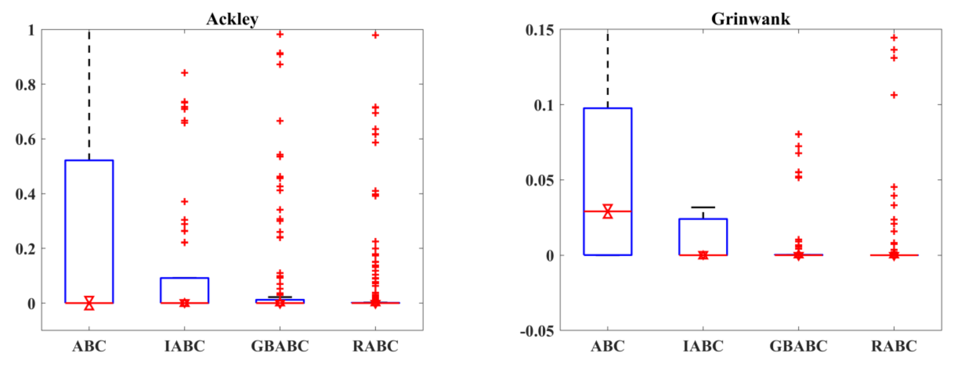
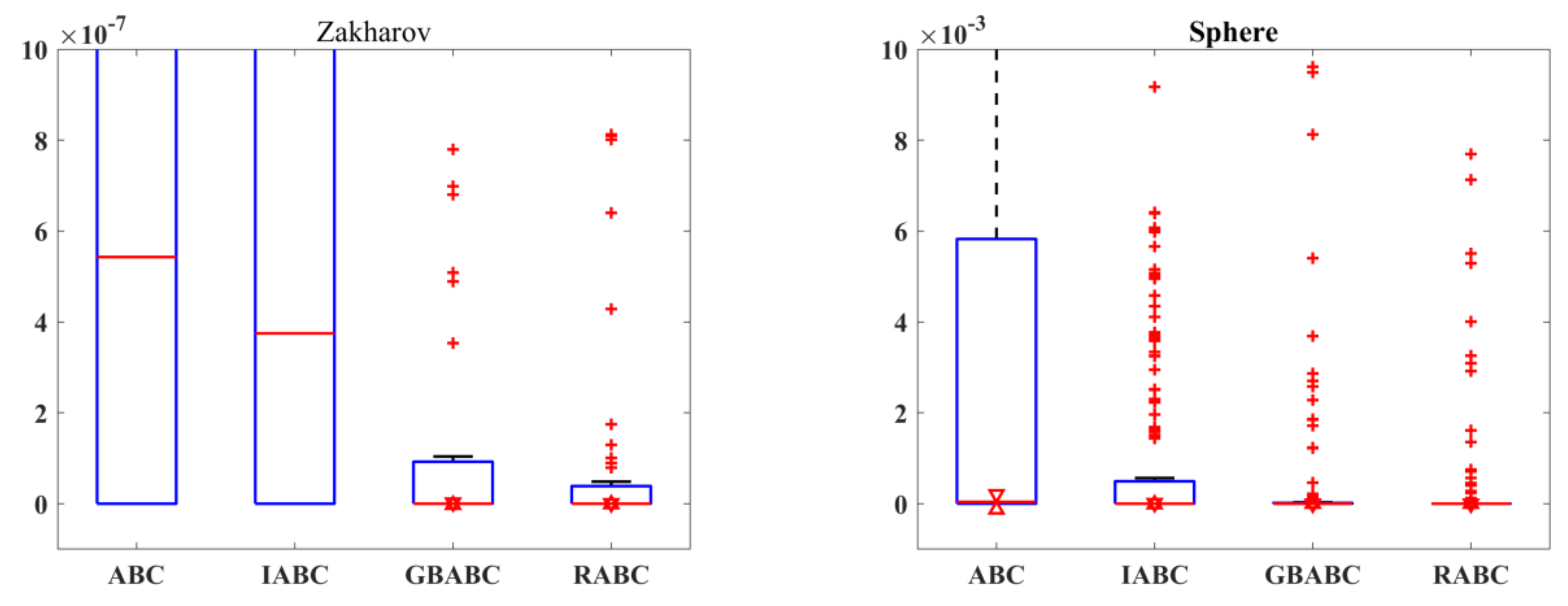
Figure 5 shows a boxplot of iterative data for four algorithms. The top and bottom edges of the boxplot indicate the 75th percentile and 25th percentile, respectively. From Figure 5, it can be further seen that the top and bottom edges of the boxplot from the RABC almost overlap, which further illustrates the fast convergence of the RABC.

4. PCP Based on ETGM(1,1)-RABC

In this section, the details of the proposed method to solve the PCP are described.

4.1. Pipeline Data

The proposed method is validated using data from a mine tailings pipeline that conveys solid–liquid mixtures. The actual wall thickness of the mine tailings pipeline is shown in Table 3. The data in Table 3 are divided into two parts. The data for the first 12 months are used for the modeling solution of the ETGM(1,1)-RABC. The data for the second 6 months are used to evaluate the accuracy of the ETGM(1,1)-RABC.

4.2. Objective Function

The objective function for the proposed method is the weighted sum of squared errors, which can be given by
min k   =   2 n φ k x ^ 0 k     x 0 k 2
where x(0) (k) is the raw data for modeling; x ^ 0 k is the predicted value; and φ (k) is the weighting coefficient, and its value is the ratio of each squared error to the sum of squared errors.

4.3. Evaluation Tool

The Taylor diagram was applied as an evaluation tool for different methods. The Taylor diagram is a graph that represents the standard deviation (STD), root mean square error (RMSE), and correlation coefficient (COR). It is more intuitive than a single graph with horizontal and vertical coordinates such as COR and RMSE. It can display the STD, RMSE, and COR of multiple variables on a two-dimensional graph, which can reflect the simulation ability of multiple models in a clear and comprehensive way [30].

4.4. Predicted Results

To validate the proposed method, GM(1,1), ETGM(1,1), ETGM(1,1)-ABC, and ETGM(1,1)-IABC are used as comparisons with ETGM(1,1)-RABC. Comparisons between GM(1,1) and ETGM(1,1) are presented, followed by comparisons of ETGM(1,1)-ABC, ETGM(1,1)-IABC, and ETGM(1,1)-RABC.

4.4.1. Comparison of GM(1,1) and ETGM(1,1)

To highlight the improvement in GM(1,1), only the comparison between GM(1,1) and ETGM(1,1) is presented here. According to the data of the mine tailing pipeline 13–18 months, the prediction results obtained by GM(1,1) and ETGM(1,1) are presented in Table 4 and Figure 6, Figure 7 and Figure 8, respectively.
Two aspects can be seen in Figure 6. On the one hand, the actual wall thickness processed by ET is smoother. On the other hand, the prediction curve obtained by ETGM(1,1) is closer to the actual wall thickness than that obtained by GM(1,1). Table 4 further illustrates that ETGM(1,1) is superior to GM(1,1). Table 4 shows that the absolute error of ETGM(1,1) is much smaller than that of GM(1,1) in months 13–16, while the absolute error of ETGM(1,1) is slightly larger than that of GM(1,1) in months 17 and 18. Figure 7 also illustrates the same situation as Table 4 on absolute error.
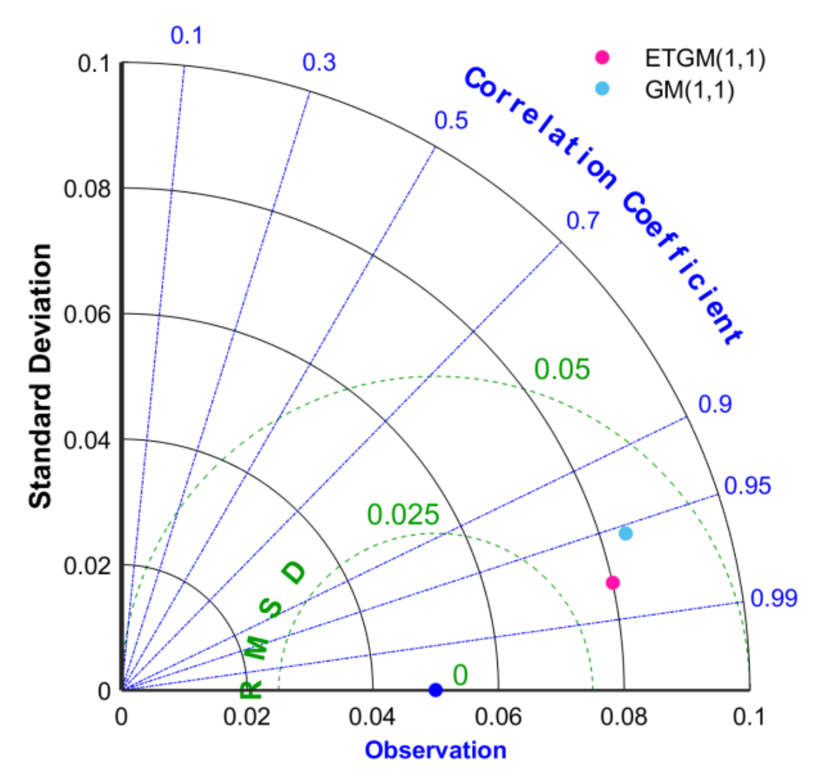
Figure 8 gives a comparison of GM(1,1) and ETGM(1,1) in view of the Taylor diagram. Figure 7 shows that the prediction accuracy of ETGM(1,1) is better than that of GM(1,1). This means that ET improves the prediction accuracy of GM(1,1).

4.4.2. Comparison of ETGM(1,1)-ABC Variants

The comparison of ETGM(1,1)-ABC, ETGM(1,1)-IABC, ETGM(1,1)-GBABC, and ETGM(1,1)-RABC is performed to highlight the role of the optimized dynamic coefficients. In this case, solving the dynamic coefficients is treated as a parametric optimization problem solved by the ABC algorithm variants, which include ABC, IABC, GBABC, and RABC. For the sake of fairness, the parameters, such as D = 1, SN = 20, limit = 20, and Maxcycle = 50, are set to be the same for all three algorithms. To ensure that the prediction result is optimal, each algorithm is run 10 times and the result with the minimum error is used as the final prediction result.
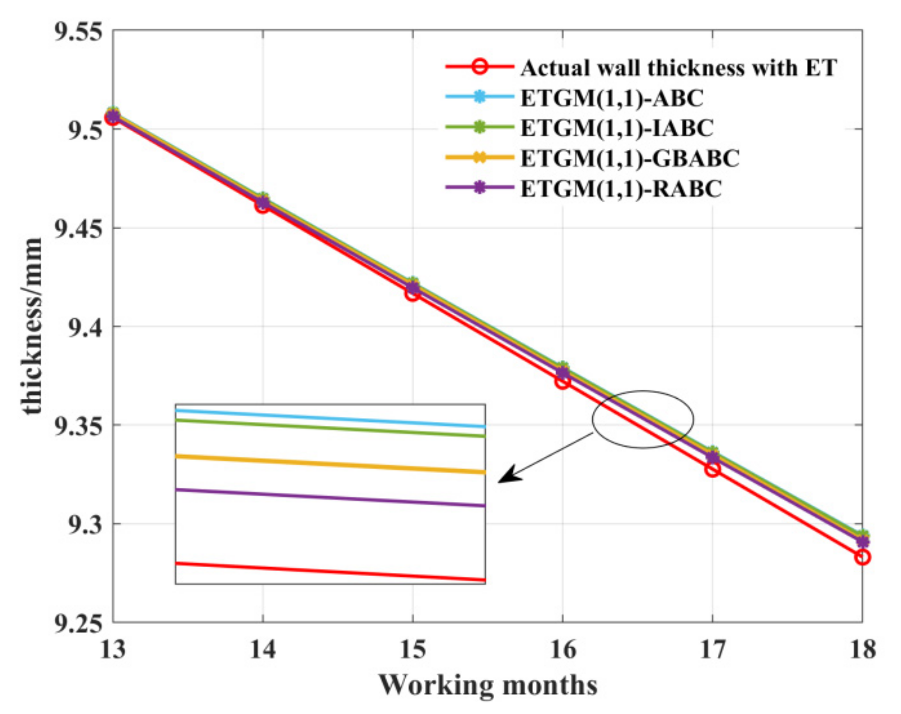
The prediction results obtained by ETGM(1,1)-ABC, ETGM(1,1)-IABC, ETGM(1,1)-GBABC, and ETGM(1,1)-RABC are shown in Figure 9 and Figure 10. Table 5 shows the prediction accuracy of the four methods.
In general, the proposed method can obtain good prediction results. From Figure 9, it can be clearly observed that ETGM(1,1)-RABC, ETGM(1,1)-GBABC, ETGM(1,1) -IABC, and ETGM(1,1)-ABC ranked first, second, third, and fourth, respectively, in terms of proximity to the actual curve. From Table 5 and Figure 10, ETGM(1,1)-RABC still ranks first in minimum absolute error.
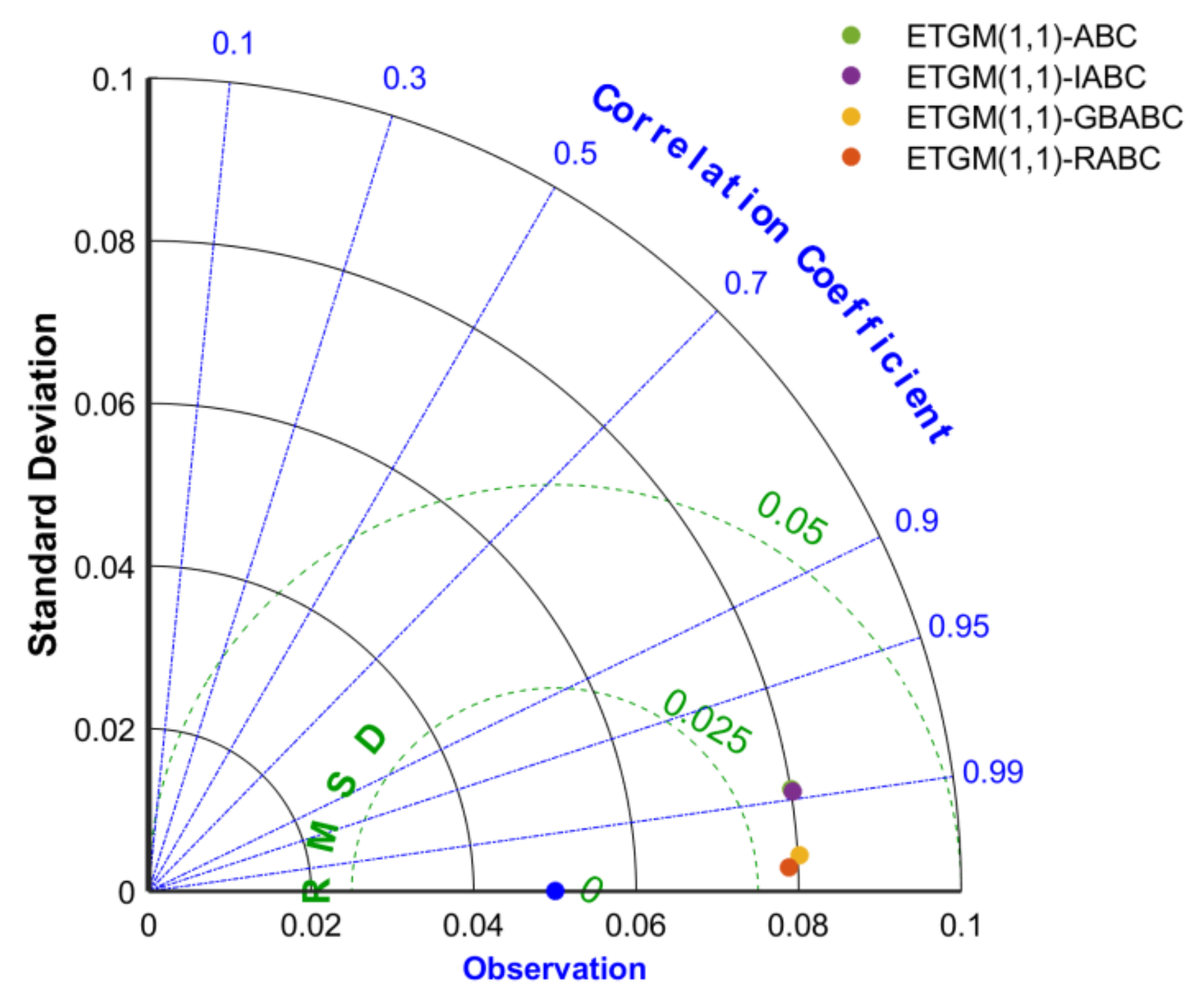
Comparing Figure 7 with Figure 11, we can observe that that the ABC and ABC variants further enhance the prediction accuracy of ETGM(1,1) for PCP. However, ETGM(1,1)-RABC still remains very competitive.

5. Conclusions

The purpose of the current study was to improve the prediction accuracy of the GM(1,1) for PCP. Based on the GM(1,1), we proposed the ETGM(1,1)-RABC method that incorporated dynamic coefficients, reformative artificial bee colony (RABC) algorithm, and exponential transform (ET); compared ETGM(1,1)-RABC with ETGM(1,1)-ABC, ETGM(1,1)-IABC, and ETGM(1,1)-GBABC; and concluded that our method was superior to the other three methods. This work demonstrates the effectiveness of our improvements to GM(1,1) for PCP. Future work will investigate the effect of other heuristic optimization algorithms on the dynamic coefficients.

Author Contributions

Methodology, H.W. and S.L.; validation, H.D., Q.C. and P.L.; writing—original draft preparation, H.D., Q.C. and P.L.; writing—review and editing, H.W. and S.L.; supervision, X.M.; funding acquisition, H.W. All authors have read and agreed to the published version of the manuscript.

Funding

This study was fully supported by Liaoning Provincial Department of Education Basic Research Projects for Higher Education Institutions, China (No. LJKZ0301); The Scientific Research Foundation of the Education Department of Liaoning Province, China (No. 2017LNQN22); Young Teachers Foundation of University of Science and Technology Liaoning, China (No. 2017QN04).

Data Availability Statement

Not applicable.

Conflicts of Interest

The authors declare no conflict of interest.

References

  1. Huang, K.; Wu, J.; Quan, K. Review on Evaluation Technology of Oil-Gas Pipelines with Corrosion Defect. Surf. Technol. 2018, 47, 116–122. [Google Scholar]
  2. Obaseki, M. Diagnostic and prognostic analysis of oil and gas pipeline with allowable corrosion rate in Niger Delta Area, Nigeria. J. Appl. Sci. Environ. Manag. 2019, 23, 927–934. [Google Scholar] [CrossRef]
  3. Li, G.D.; Wang, C.H.; Yamaguchi, D.; Nagai, M.; Masuda, S. A study on the corrosion process of gas pipeline applying grey dynamic model. Int. J. Reliab. Saf. 2010, 4, 1–15. [Google Scholar] [CrossRef]
  4. Shaik, N.B.; Pedapati, S.R.; Othman, A.R.; Bingi, K.; Abd Dzubir, F.A. An intelligent model to predict the life condition of crude oil pipelines using artificial neural networks. Neural Comput. Appl. 2021, 33, 14771–14792. [Google Scholar] [CrossRef]
  5. Wen, K.; He, L.; Liu, J.; Gong, J. An optimization of artificial neural network modeling methodology for the reliability assessment of corroding natural gas pipelines. J. Loss Prev. Process Ind. 2019, 60, 1–8. [Google Scholar] [CrossRef]
  6. Shaik, N.B.; Pedapati, S.R.; Taqvi, S.A.A.; Othman, A.R.; Abd Dzubir, F.A. A feed-forward back propagation neural network approach to predict the life condition of crude oil pipeline. Processes 2020, 8, 661. [Google Scholar] [CrossRef]
  7. Liao, D.; Zhang, L.; Tao, G. Study on corrosion rate of buried gas steel pipeline in Nanjing based on the GM (1, N) optimization model. IOP Conf. Ser. Mater. Sci. Eng. 2019, 490, 022025. [Google Scholar] [CrossRef]
  8. Gao, J.; Hao, B. Prediction of Submarine Pipeline Corrosion Based on the Improved Grey Prediction Model. J. Phys. Conf. Ser. 2021, 1894, 012106. [Google Scholar] [CrossRef]
  9. Zhengshan, L.U.O.; Hongwei, Y. GM-RBF model based error compensation for prediction of submarine pipeline corrosion. China Saf. Sci. J. 2018, 28, 96. [Google Scholar]
  10. Deng, Z.; Ding, H.; Miao, K.; Zhang, X.; Xu, T.; Li, G. Grey Relational Analysis and Fuzzy Neural Network Method for Predicting Corrosion Rate of Marine Pipeline. Int. J. High. Educ. Teach. Theory 2021, 2, 210. [Google Scholar]
  11. Jiang, Y.; Wang, L.; Liu, Y.T.; Zhang, Y. Combined Grey Prediction and Neural Network Model for Oil and Gas Pipeline Wall Thinning. J. Phys. Conf. Ser. 2021, 2033, 012210. [Google Scholar] [CrossRef]
  12. Peng, S.; Zhang, Z.; Liu, E.; Liu, W.; Qiao, W. A new hybrid algorithm model for prediction of internal corrosion rate of multiphase pipeline. J. Nat. Gas Sci. Eng. 2021, 85, 103716. [Google Scholar] [CrossRef]
  13. Li, X.; Zhang, L.; Khan, F.; Han, Z. A data-driven corrosion prediction model to support digitization of subsea operations. Process Saf. Environ. Prot. 2021, 153, 413–421. [Google Scholar] [CrossRef]
  14. Peng, X.; Anyaoha, U.; Liu, Z.; Tsukada, K. Analysis of magnetic-flux leakage (MFL) data for pipeline corrosion assessment. IEEE Trans. Magn. 2020, 56, 1–15. [Google Scholar] [CrossRef]
  15. Abyani, M.; Bahaari, M.R. A new approach for finite element based reliability evaluation of offshore corroded pipelines. Int. J. Press. Vessel. Pip. 2021, 193, 104449. [Google Scholar] [CrossRef]
  16. Deif, S.; Daneshmand, M. Multiresonant chipless RFID array system for coating defect detection and corrosion prediction. IEEE Trans. Ind. Electron. 2019, 67, 8868–8877. [Google Scholar] [CrossRef]
  17. Gao, H.; Shi, Y.; Pun, C.M.; Kwong, S. An improved artificial bee colony algorithm with its application. IEEE Trans. Ind. Inform. 2018, 15, 1853–1865. [Google Scholar] [CrossRef]
  18. Brezočnik, L.; Fister, I.; Podgorelec, V. Swarm intelligence algorithms for feature selection: A review. Appl. Sci. 2018, 8, 1521. [Google Scholar] [CrossRef] [Green Version]
  19. Li, C.; Gao, H.; Qiu, J.; Yang, Y.; Qu, X.; Wang, Y.; Bi, Z. Grey model optimized by particle swarm optimization for data analysis and application of multi-sensors. Sensors 2018, 18, 2503. [Google Scholar] [CrossRef] [Green Version]
  20. Squires, M.; Tao, X.; Elangovan, S.; Gururajan, R.; Zhou, X.; Acharya, U.R. A novel genetic algorithm based system for the scheduling of medical treatments. Expert Syst. Appl. 2022, 195, 116464. [Google Scholar] [CrossRef]
  21. Deng, W.; Shang, S.; Cai, X.; Zhao, H.; Song, Y.; Xu, J. An improved differential evolution algorithm and its application in optimization problem. Soft Comput. 2021, 25, 5277–5298. [Google Scholar] [CrossRef]
  22. Guo, C.; Tang, H.; Niu, B. Evolutionary state-based novel multi-objective periodic bacterial foraging optimization algorithm for data clustering. Expert Syst. 2022, 39, e12812. [Google Scholar] [CrossRef]
  23. Rivera, G.; Coello, C.A.C.; Cruz-Reyes, L.; Fernandez, E.R.; Gómez Santillán, C.G.; Rangel-Valdez, N. Preference incorporation into many-objective optimization: An Ant colony algorithm based on interval outranking. Swarm Evol. Comput. 2022, 69, 101024. [Google Scholar] [CrossRef]
  24. Xiao, X.; Guo, H.; Mao, S. The modeling mechanism, extension and optimization of grey GM (1, 1) model. Appl. Math. Model. 2014, 38, 1896–1910. [Google Scholar] [CrossRef]
  25. Zhang, D.L.; Ying-Gan, T.; Xin-Ping, G. Optimum design of fractional order PID controller for an AVR system using an improved artificial bee colony algorithm. Acta Autom. Sin. 2014, 40, 973–979. [Google Scholar] [CrossRef]
  26. Bian, G.X.; Xu, Y.M. Improvement of GM (1, 1) model based on data transformation. J. Geomat. 2019, 44, 122–124. [Google Scholar]
  27. Cheng, M.; Li, J.; Liu, Y.; Liu, B. Forecasting clean energy consumption in China by 2025: Using improved grey model GM (1, N). Sustainability 2020, 12, 698. [Google Scholar] [CrossRef] [Green Version]
  28. XieXun, Q.I.N.; WenBin, L.I.U.; LiangChao, C. Pipeline corrosion prediction based on an improved artificial bee colony algorithm and a grey model. J. Beijing Univ. Chem. Technol. 2021, 48, 74. [Google Scholar]
  29. Zhou, X.; Wu, Z.; Wang, H. Gaussian bare-bones artificial bee colony algorithm. Soft Comput. 2016, 20, 907–924. [Google Scholar] [CrossRef]
  30. Taylor, K.E. Summarizing multiple aspects of model performance in a single diagram. J. Geophys. Res. Atmos. 2001, 106, 7183–7192. [Google Scholar] [CrossRef]
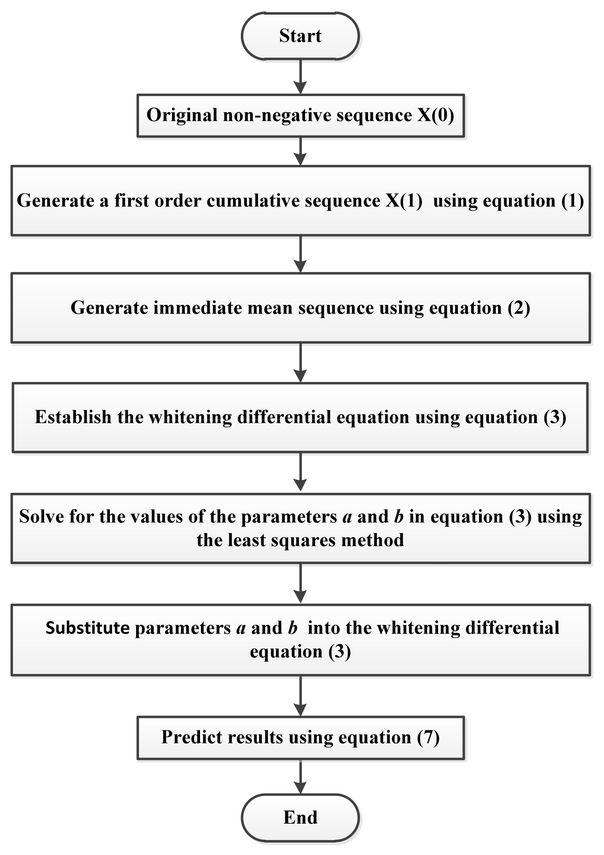
Figure 1. Flowchart of the GM(1,1).
Axioms 11 00289 g001
Figure 2. The schematic of the proposed method.
Axioms 11 00289 g002
Figure 3. Error in the background values.
Axioms 11 00289 g003
Figure 4. Convergence obtained by the ABC, IABC, GBABC, and RABC algorithms.
Axioms 11 00289 g004
Figure 5. Box plot obtained by the ABC, IABC, GBABC, and RABC algorithms.
Axioms 11 00289 g005aAxioms 11 00289 g005b
Figure 6. Prediction curve for wall thickness.
Axioms 11 00289 g006
Figure 7. Absolute error curves.
Axioms 11 00289 g007
Figure 8. Accuracy comparison of GM(1,1) and ETGM(1,1) using the Taylor diagram.
Axioms 11 00289 g008
Figure 9. Prediction curve for wall thickness.
Axioms 11 00289 g009
Figure 10. Absolute error curve.
Axioms 11 00289 g010
Figure 11. Accuracy comparison of four methods using the Taylor diagram.
Axioms 11 00289 g011
Table 1. Benchmark functions.
FunctionNameDefinition DomainOptimal Value
F1Ackley(−15, 30)0
F2Griewank(−600, 600)0
F3Zakharov(−5, 10)0
F4Sphere(−100, 100)0
Table 2. Mean and std obtained by the ABC, IABC, GBABC, and RABC algorithms.
Function ABCIABCGBABCRABC
F1Mean
Std
6.33345e-13
4.89751e-14
1.42997 e-13
1.00486 e-14
9.85936e-14
8.65746e-15
8.26357e-14
4.29453e-15
F2Mean
Std
4.01418e-12
3.77788e-12
8.13825e-14
8.65482e-15
5.10703e-15
5.80934e-15
1.16573 e-15
2.35514 e-16
F3Mean
Std
8.04328e-15
7.47394e-15
1.8455 e-15
1.5451 e-16
1.14164e-15
5.13749e-17
1.07917e-15
8.23919e-17
F4Mean
Std
7.29812e-15
8.75926e-17
1.96226 e-15
1.98675 e-16
1.34151e-15
1.24779e-17
1.10285e-15
1.03897e-17
Table 3. Actual wall thickness for the mine tailings pipeline.
Working MonthsActual Wall Thickness/mmWorking MonthsActual Wall Thickness/mm
110.03109.64
210.01119.58
39.95129.53
49.92139.51
59.85149.49
69.82159.45
79.76169.38
89.71179.31
99.69189.27
Table 4. The predicted results obtained by ETGM(1,1) and GM(1,1).
Working MonthsActual Wall Thickness/mmETGM(1,1)GM(1,1)
Predicted Value/mmAbsolute Error/mmPredicted Value/mmAbsolute Error/mm
139.51 (9.506)9.50850.00259.49110.0189
149.49 (9.461)9.46520.00429.44570.0443
159.45 (9.417)9.42220.00529.40050.0495
169.38 (9.372)9.37940.00749.35560.0244
179.31 (9.328)9.33670.00879.31080.0008
189.27 (9.283)9.29430.01139.26630.0037
Table 5. The predicted results obtained by four methods.
Working Months 131415161718
Actual Wall Thickness with ET 9.5069.4619.4179.3729.3289.283
ETGM(1,1)-ABCPredicted value/mm9.50859.46489.42239.37909.33699.2939
Absolute error/mm0.00250.00380.00530.00700.00890.0109
ETGM(1,1)-IABCPredicted value/mm9.50849.46479.42229.37899.33679.2938
Absolute error/mm0.00240.00370.00520.00690.00870.0108
ETGM(1,1)-GBABCPredicted value/mm9.50759.46369.42089.38429.33489.2915
Absolute error/mm0.00150.00260.00380.00520.00680.0085
ETGM(1,1)-RABCPredicted value/mm9.50669.46269.41989.37629.33389.2907
Absolute error/mm0.00060.00160.00280.00420.00580.0077
Publisher’s Note: MDPI stays neutral with regard to jurisdictional claims in published maps and institutional affiliations.