Article

Volatility Co-Movement between Bitcoin and Stablecoins: BEKK–GARCH and Copula–DCC–GARCH Approaches

1
Department of Accounting, Ming Chuan University, 250 Zhong Shan N. Rd., Sec. 5, Taipei 111, Taiwan
2
Department of Accounting, Feng Chia University, Taichung City 407102, Taiwan
*
Author to whom correspondence should be addressed.
Axioms 2022, 11(6), 259; https://doi.org/10.3390/axioms11060259
Submission received: 26 March 2022 / Revised: 16 May 2022 / Accepted: 22 May 2022 / Published: 29 May 2022
(This article belongs to the Special Issue Applied Mathematics in Finance and Economics)

Abstract

:
This paper aims to investigate and measure Bitcoin and the five largest stablecoin market volatilities by incorporating various range-based volatility estimators to the BEKK- GARCH and Copula-DCC-GARCH models. Specifically, we further measure Bitcoins’ volatility related to five major stablecoins and examine the connectedness between Bitcoin and the stablecoins. Our empirical findings document that the connectedness between Bitcoin and stablecoin market volatility behaviors exhibits the presence of stable interconnection. This study is of particular importance since it is crucial for market participation in the ongoing crypto assets to be informed about both the volatility patterns of major cryptocurrencies and the relative volatility of Bitcoin against the stablecoin markets. Eventually, we find that there is no systematic evidence for the various parity deviations of the stablecoins that are profoundly impacted by Bitcoin volatility. Thus, Bitcoin and the largest stablecoin Tether could stabilize together. However, Bitcoin shall not be generalized to other stablecoins in terms of stability results.
MSC:
91B84; 62G32; 91G80; 62H20

1. Introduction

In the past year, USD-pegged stablecoins streaming on public blockchains have been more attractive and seen explosive growth. Moreover, the growing pieces of literature on the price and volatility dynamics of cryptocurrency markets have attracted widespread attention to the fluctuation in Bitcoin as well as stablecoin prices. The crypto assets may also support a more inclusive financial system through the growth of decentralized finance (Defi). Stablecoins play a crucial role in the decentralized financial system in that their value is typically pegged to fiat currencies, (e.g., USD and CNY), or two precious metals, (e.g., gold and silver) and stablecoins, and their growth could fluctuate innovations in the digital asset economy. Stablecoins are designed as an alternative to conventional cryptocurrencies. Regarding more inclusive payment and financial systems, stablecoins have the potential role to fluctuate growth and innovation in payment systems, allowing for faster, cheaper payments. Additionally, the stablecoins are always decentralized and bridge fiat currencies with traditional digital currencies due to their pegging mechanism. Unlike conventional cryptocurrencies, stablecoins have value-preserving properties and could hedge risk for other volatile assets during the market crash, such as the stablecoin gain as major cryptocurrencies (Bitcoin and Ether) fall after Russia attacks Ukraine. According to Reuters, stablecoins, which are digital tokens pegged to risk-free currencies such as the US dollar, held profits on time during a sell-off in risky assets such as stocks and Bitcoin after Russia’s full-scale invasion of Ukraine. (https://www.reuters.com/technology/stablecoins-gain-bitcoin-ether-fall-after-russia-invades-ukraine, accessed on 24 February 2022).
According to a Wall Street Journal report (See https://www.wsj.com/livecoverage/russia-ukraine-latest-news/card/ukrainians-buy-dollar-pegged-stablecoin-amid-russian-attack-vGCCIQbH4CQx3Tl4V5D1, accessed on 25 February 2022), Ukrainians buy dollar-pegged stablecoin amid the Russian invasions. Post the Russia–Ukraine war, particularly, the market demand for pegged-stablecoins for low-volatility crypto asset instruments has rapidly accelerated the development of stablecoins. Sidorenko [1] also points out that the crypto asset market trend is moving towards the direction of converting fund flow to several representative low volatile cryptocurrencies. The decentralized stablecoins are also designed to be the fiat-collateralized digital-tokens maintaining a fiat currency reserve to exchange market or safe-haven assets, see also Wang et al. [2]; Xie et al. [3]. As their name indicates, collateralized stablecoins are introduced to offer price stability against the relatively high volatile cryptocurrencies to hedge the risk of financial market crashes, such as the COVID-19 pandemic, and the Russia-Ukraine war. Thus, two questions naturally arise:
(1)
How can stablecoins stabilize cryptocurrencies? What potential role will stablecoins perform in the violent price fluctuations in conventional cryptocurrencies?
(2)
How do they play the roles of the gold- or USD-pegged stablecoins as safe-havens, diversifiers, or hedges against conventional cryptocurrencies during the financial crisis?
To highlight the development of the Fintech ecosystem, the study makes two major contributions. Firstly, the usage of additional information is linked to closing and additionally low and high prices in its estimation of the BEKK and Copula–DCC GARCH models. These models are commonly used to capture the volatility co-movement across the cryptocurrencies and improve the empirical estimation of the covariance matrix of volatilities. Secondly, the other contribution is to provide fresh, insightful arguments to this increasing attention in research regarding their embedded exchange rate stabilization mechanisms, and then demonstrate conditional correlations and volatility spillovers between Bitcoin and the top five stablecoin markets.
To the best of our knowledge, this is the pioneering literature to investigate the Bitcoin range-based volatility linkages across the five major stablecoin markets and discuss whether the volatility of stablecoins is driven by the volatility jump of Bitcoin. From a practical perspective, this issue is more important because closing prices are widely available with a corresponding daily close, high, and low price for current financial markets.
The rest of the paper is organized as follows. Section 2 reviews the related literature and Section 3 introduces the methods and econometric model. Section 4 performs the competing econometric models and analyzes the estimation results, and Section 5 concludes.

2. Literature Review

Broadly speaking, Ito et al. [4] document that stablecoins are designed to be a stabilization mechanism backed by either fiat currencies or precious metals under a fixed exchange rate regime among cryptoassets. To reduce the excessive volatility of cryptocurrencies, an effective mechanism is to peg their value to fiat currencies. Lyons and Viswanath-Natraj [5] observed that parity deviations of the major stablecoin Tether are deeply impacted by Bitcoin volatility. As previous studies empirically investigated, Griffin and Shams [6] reported that the timing of Tether purchases following market downturns lead to Bitcoin’s dramatic price rise. Furthermore, other works of stablecoins have shown their safe haven features, (e.g., Wang et al. [2]) and their price stabilization mechanisms in the light of pegged exchange rate regimes for fiat currencies, (e.g., Lyons et al. [5]). On the contrary, is the stablecoin potentially employed to boost Bitcoin prices? Wei [7] investigated the largest stablecoin, Tether, but he had not found any evidence that Tether’s manipulation led to the 2017 Bitcoin rally. In addition, Kristoufek [8] also found no evidence of stablecoins flourishing at the prices of other cryptocurrencies. Amid the rapid growth of the new digital financial market ecosystem, the priority for a central bank digital currency (CBDC) is to preserve ready public access to government-issued, risk-free currency in the digital financial ecosystem. Thus, CBDCs could coexist with stablecoins. Theoretically, Tether based on blockchain is a peer-to-peer payment and transaction cryptocurrency. However, it is the most secure stablecoin with a value pegged to the US dollar. In simple terms, a US Tether token is one US dollar at all times. Similarly, Lyons and Viswanath-Natraj [9] show no systematic evidence that Tether issuances are impacted by the prices of major non-stable cryptocurrencies, (e.g., Bitcoin and Ethereum). Given the highly volatile nature of cryptocurrencies, stablecoins are developed as the stabilization mechanism to maintain a stable market value as they are pegged to another safe-haven asset (Wang et al. [7]; Xie et al. [3]). Given the growing interest in cryptocurrencies, a few pieces of literature have investigated whether stablecoins are truly diversifiers or stable. Considering the stability of stablecoins, Hoang et al. [10] document that Bitcoin is a likely source of excessively volatile stablecoins and uncover significant evidence that stablecoins are the driver of the excessive volatility of Bitcoin. Moreover, a new strand of study has been examined by Grobys et al. [11], who found strong evidence that stablecoin volatility spills over to Bitcoin. Considering the rapid development of stablecoins in the Fintech system, it is beneficial to expand the frontiers of knowledge of stablecoins. Perhaps surprisingly, most pieces of literature only investigate the stablecoins’ response to sudden shocks in Bitcoin’s price volatility or the interplay between stablecoins and Bitcoin. The current work looks to contribute to the studies by analyzing the interactions between the stabilities of the top five stablecoins. This study suggests that the stabilization mechanism plays an important role in interpreting the volatility connectedness between stablecoins. Accordingly, we attempt to fill this gap and aim to expand the scope of research of Hoang and Baur [10] and Grobys et al. [11] and examine whether there is the existence of volatility spillovers among Bitcoin and stablecoins. To investigate the possibility of volatility transmission, we apply the VAR–BEKK–GARCH and Copula–DCC–GARCH models for the daily ranged-based and GARCH volatility estimation of six major cryptocurrencies including Bitcoin, Tether, USD Coin, Binance, Terra, and Dai. The BEKK model was proposed by Baba et al. (1990) [12] and Engle and Kroner (1995) [13]. In practice, the VAR–BEKK–GARCH model is empirically applied in this work, also named the flexible multivariate GARCH (MGARCH) specifications. Empirically, we also use the VAR Granger causality models to investigate the range-based volatility interactions among Bitcoin and the largest five stablecoins. These models can be used to simultaneously predicate the volatility spillover effect across the major cryptocurrencies under considerable information related to open, high, low, and closing prices in the BEKK–GARCH and Copula–DCC–GARCH estimations (see, e.g., Fiszeder [14]; Tan et al., [15]; Brandt et al. [16]; Li et al. [17]; Fiszeder et al. [18]; Molnár [19]; Jacob et al. [20], Todorova et al. [21]). Similarly, the multivariate GARCH methodology provides further interpretations of the innovation shock transmission among two or more markets. The BEKK and DCC–GARCH models are widely used because they are the most popular classes of competing models, and the multivariate GARCH models often capture the volatility dynamics of financial time series (see, e.g., Bauwens et al. [22]; Block et al. [23]; Mensi et al., [24]). Our paper uncovers the interactions of volatilities between the leading Bitcoin and stablecoin markets. Furthermore, our paper contributes to increasing interest in research on emerging Fintech ecosystems.

3. Methodology and Econometric Model

We introduce the following measures of the stability of stablecoins:

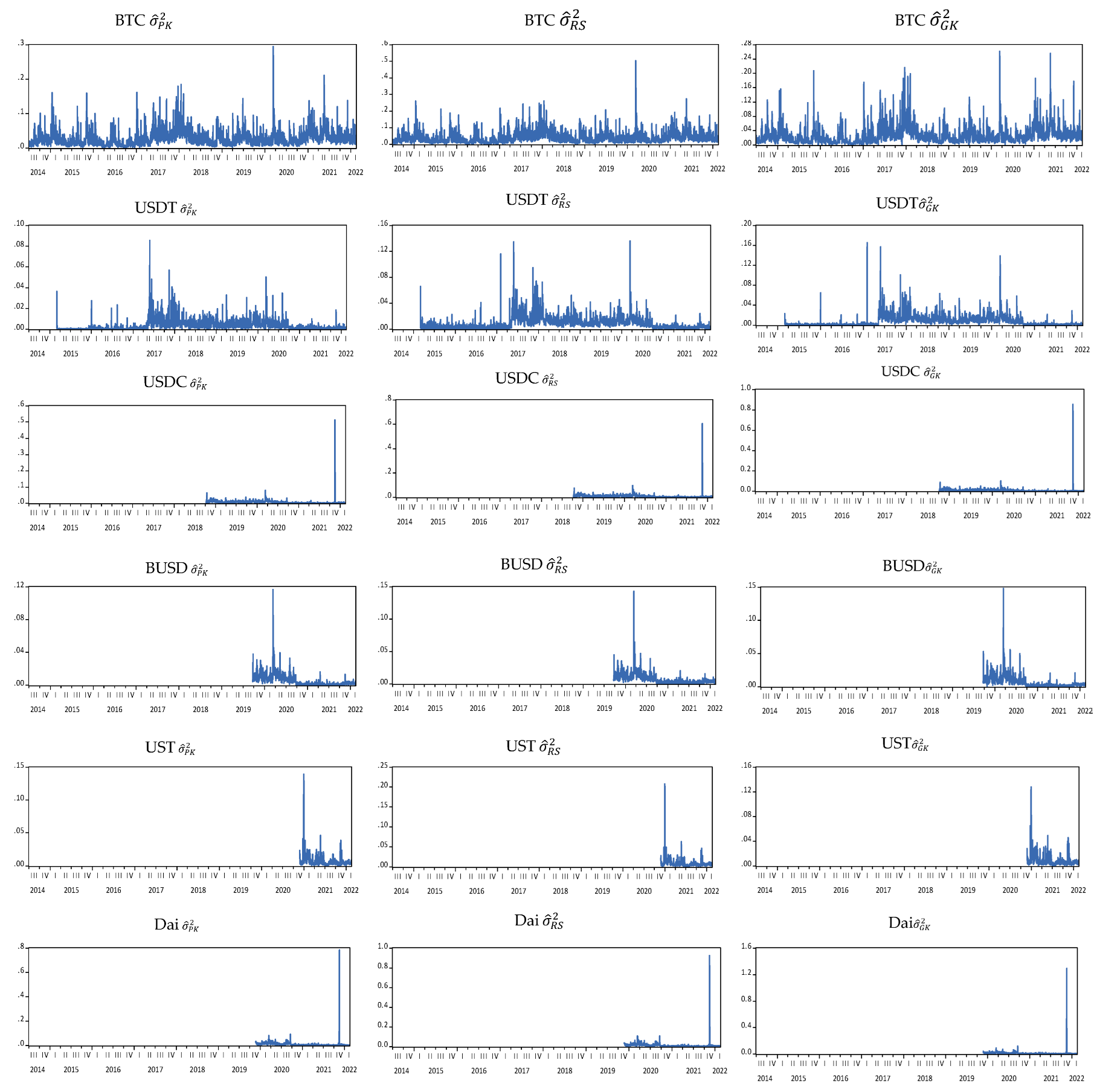
3.1. Range-Based Volatility for Various Variance Estimators

Considering a probability space ( Ω , ,   P ) defined as a right-continuous filtration ( t ) t > 0 , it satisfies the usual conditions of completeness. One can consider a financial market wherein heterogeneous agents bid or ask for cryptocurrencies and represent the price process of the cryptocurrency by ( S = S t , t ≥ 0). The cryptocurrency price under the physical probability measure P, its price whose return dynamics can be expressed as:
d S t S t = μ d t + σ d B t
where μ and σ denote the instantaneous expected rate of return and the continuous volatility, respectively. B t denotes the standard Brownian motion. By Ito’s lemma, the cryptocurrency’s price after taking the natural logarithm is given by:
d l n S t = ( μ 1 2 σ 2 ) d t + σ d B t
Several alternative variance estimators have been proposed to estimate the parameters under this hypothesis about the distribution of a cryptocurrency price.
Assuming C t , O t , H t , L t represent the log of the closing, opening, highest, and lowest price on date t, respectively. σ ^ is the volatility to be estimated. Parkinson [25] develop the first range-based estimator and employed the high and low values to measure the variance which satisfies
σ ^ P K 2 = 0.3607 ( H t L t ) 2
where the factor 0.3607 is equal to 1 4 l n 2 .
Afterward, Garman and Klass [26] expanded the Parkinson’s method by incorporating the opening and closing prices into the equation. Rogers and Satchell [27] release this restriction that includes a nonzero drift term and develops an estimator and hence is theoretically more efficient than the range-based estimator (3). Their volatility estimator is shown below
σ ^ R S 2 = ( H t C t ) ( H t O t ) + ( L t C t ) ( L t O t )
Alternative Range-Based Volatility Measures.
An alternative volatility proxy we consider is the historical volatility estimator of Garman and Klass [26]. This study hence introduces their practical range-based volatility estimators as following
σ ^ G K 2 = 1 2 ( H t L t ) 2 ( 2 l n 2 1 ) ( C t O t ) 2

3.2. The BEKK–GARCH Model with Low, High, and Closing Prices

As the previous literature mentioned, Parkinson (1980) [25] was the first to the development of the range-based in measuring volatility, which is widely used to identify volatility behavior in the financial market. Parkinson found the daily volatility estimator, (i.e., PARK estimator) based on the postulate that the intra-daily prices follow Brownian motion given as Equation (2). This study incorporates the GARCH model of the PARK range to identify shocks via time-varying volatility. In the previous study, the specification is also called GARCH–PARK–R model. Consider the covariance stationary time series { R P K } and PARK estimator is given by:
R P K = 1 4 l n 2 ( H t L t )
where R P K represents the PARK-range of the crypto asset at time t. Furthermore, let R P K ≥ 0 for all t and that P ( R P K , t < δ| R P K , t + 1 , R P K , t + 2 , …) > 0 for any δ > 0 and for all t.
This paper investigates the volatility spillovers among six major cryptocurrencies including Bitcoin, Tether, USD Coin, Binance, Terra, and Dai, which are substituted into the mean equation outlined below. Empirically, the VAR (1)—BEKK–GARCH (1, 1) methodology proposed by Engle and Kroner [13] is applied to examine the volatility linkages among these six variables. The conditional mean of the bivariate VAR (1)-GARCH (1, 1) model can be given as the following specification:
{ R P K , t = μ + Φ R P K , t 1 + ε t ε t = H t 1 / 2   ξ t
where, R P K , t = ( R P K , t B , R P K , t S )′ represents a 2 × 1 vector for each pair of Bitcoin volatility against stablecoins volatilities (Tether, USD Coin, Binance USD, Terra USD, and Dai). Φ represent a (2 × 2) matrix of coefficients of the form Φ = ( ϕ 1 0 0 ϕ 2 ), and ε t = ( ε t B , ε t s )′ is distributed as the vector of the random noises of the conditional mean equations for Bitcoin and stablecoin volatilities, respectively. In addition, H t 1 / 2 refers to a symmetric positive definite (2 × 2) matrix and ξ t = ( ξ t B ,   ξ t s ) is the vector of i.i.d. random noises. R P K , t also indicates the estimators based on Equation (3) to measure these variables. For the sake of exposition, the conditional variances of the VAR (1)—BEKK–GARCH (1, 1), and then the covariance matrix can be given by:
H t = C C + A ( ε t 1 ε t 1 ) A + B H t 1 B
where H t denotes the variance-covariance matrix, A, B represent the square coefficient matrices that are diagonalized to ensure covariance stationarity, and C denotes an upper triangular matrix. Therefore, the representative matrices of parameters are C , A, and B and can be written as follows:
C = ( c 11 0 c 21 c 22 ) ,   A = ( α 11 α 12 α 21 α 22 ) ,   B = ( β 11 β 12 β 21 β 22 )
Afterward, the unrestricted model in bivariate BEKK form is given by
( h 11 , t h 12 , t h 21 , t h 22 , t ) = ( c 11 0 c 21 c 22 ) ( c 11 0 c 21 c 22 ) +   ( α 11 α 12 α 21 α 22 ) ( ε 1 , t 1 2 ε 1 , t 1   ε 2 , t 1 ε 1 , t 1 ε 2 , t 1 ε 2 , t 1 2 ) ( α 11 α 12 α 21 α 22 ) + ( β 11 β 12 β 21 β 22 ) ( h 11 , t 1 h 12 , t 1 h 21 , t 1 h 22 , t 1 ) ( β 11 β 12 β 21 β 22 )
For the sake of simplifying, we follow Katsiampa [28], and then the triangular parameter matrix can be taken the form as
h 11 , t = c 11 2 + α 11 2 ε 1 , t 1 2 + β 11 2 h 11 , t 1 h 22 , t = c 12 2 + c 22 2 + α 12 2 ε 1 , t 1 2 + 2 α 12 α 22 ε 1 , t 1 ε 2 , t 1 + α 22 2   ε 2 , t 1 2 + β 12 2 h 11 , t 1 + 2 β 12 β 22 h 12 , t 1 + β 22 2 h 22 , t 1 h 12 , t = c 12 c 22 + α 11 α 12 ε 1 , t 1 2 + α 11 α 22 ε 1 , t 1 ε 2 , t 1 + β 11 β 22 h 12 , t 1
The matrices A and B also depict the estimators indicating the impacts of the ARCH effect (short-term volatility shocks) and the GARCH effect (long-run volatility shocks), respectively. Let us postulate that the conditional variance for each price changes, h i j , t follows a bivariate GARCH process, and can be expressed as
h i j , t = c i j + α i j   ε i j , t 1 2 + β i j   h i j , t 1
where α i j is the short-term persistence, or ARCH effect, of shocks to changes i, β i j denotes the GARCH effect, and α i j + β i j measures the long-term persistence or volatility clustering.
The joint Gaussian log-likelihood function for T number of observations is postulated to the conditional distribution of these variables. Consequently, estimating the VAR (1)-BEKK–GARCH (1, 1) model, can be performed by the quasi-maximum likelihood (QML) methodology. In general, the Gaussian log-likelihood function for example k = 2 in the bivariate model is given as follows
l o g   L = 1 2 t = 1 T [ k l o g ( 2 π ) + ε t H t 1 ε t + l n | H t | ]

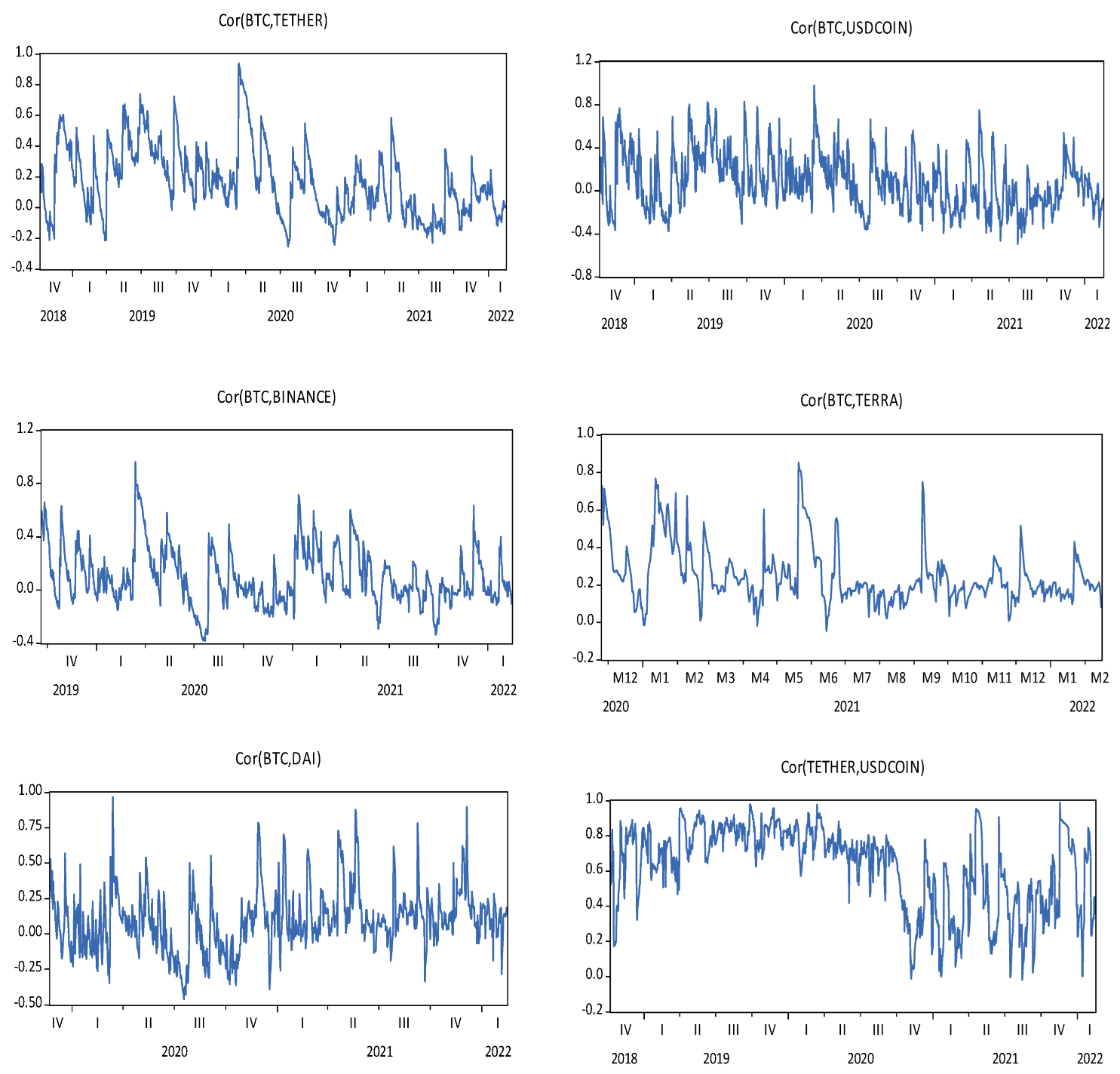
3.3. The Copula–DCC–GARCH Model

To capture the dynamic conditional correction between cryptocurrencies, the dynamic relationship is analyzed with the usage of a Copula–DCC–GARCH model for daily ranged-based volatility. In this paper, employing the residuals { ε t } which are obtained from the VAR model, we estimate the conditional covariance matrix with a Copula–DCC–GARCH model, expressed by Equation (14), which can capture the asymmetric leptokurtic behavior of cryptoassets. Hereafter, the specification of the dynamic conditional correction model is given as follows:
H t = D t R t D t
where
D t = diag ( v t ) ,   v t = ( h 1 , t 1 / 2 h N , t 1 / 2 )
Similarly, the conditional variance estimation for Formula (15) follows the preceding Equation (12) of the bivariate BEKK–GARCH model.
R t = Q t * 1 Q t Q t * 1
Q t * = diag ( Q t 1 / 2 ) ,   where   Q t = ( q 11 , t q N N , t )
As the square matrix of order N exhibits symmetric and positive definite Q t ( q i j , , t ) can be expressed in the form proposed in Equation (18).
Q t = ( 1 a b ) Q ¯ + a u t 1 u t 1 T + b Q t 1  
where Q ^ t denotes the N × N matrix consisting of the unconditional covariance of u i , t , and u i , t / h i , t ~ s k e w t v ; a and b are the estimated parameters and non-negative scalar parameters satisfying a + b < 1. The model parameters were estimated via the quasi-maximum likelihood (QML) approach and the log-likelihood function is also specified as
l o g L = t = 1 T 1 2 ( n ln π + ln ( d e t H t ) + u t H t 1 u t T )
The definition of residuals u i , t joint distribution expands the conventional DCC proposed by Engle [29], through copulas, which can describe the data with more flexibility once copulas are estimated from marginal distribution. Subsequently, the copula models we consider here are student-t copulas which are applied to predict the time-varying correlation matrix of the DCC model (Righi, et al. [30]; Block et al. [23]).

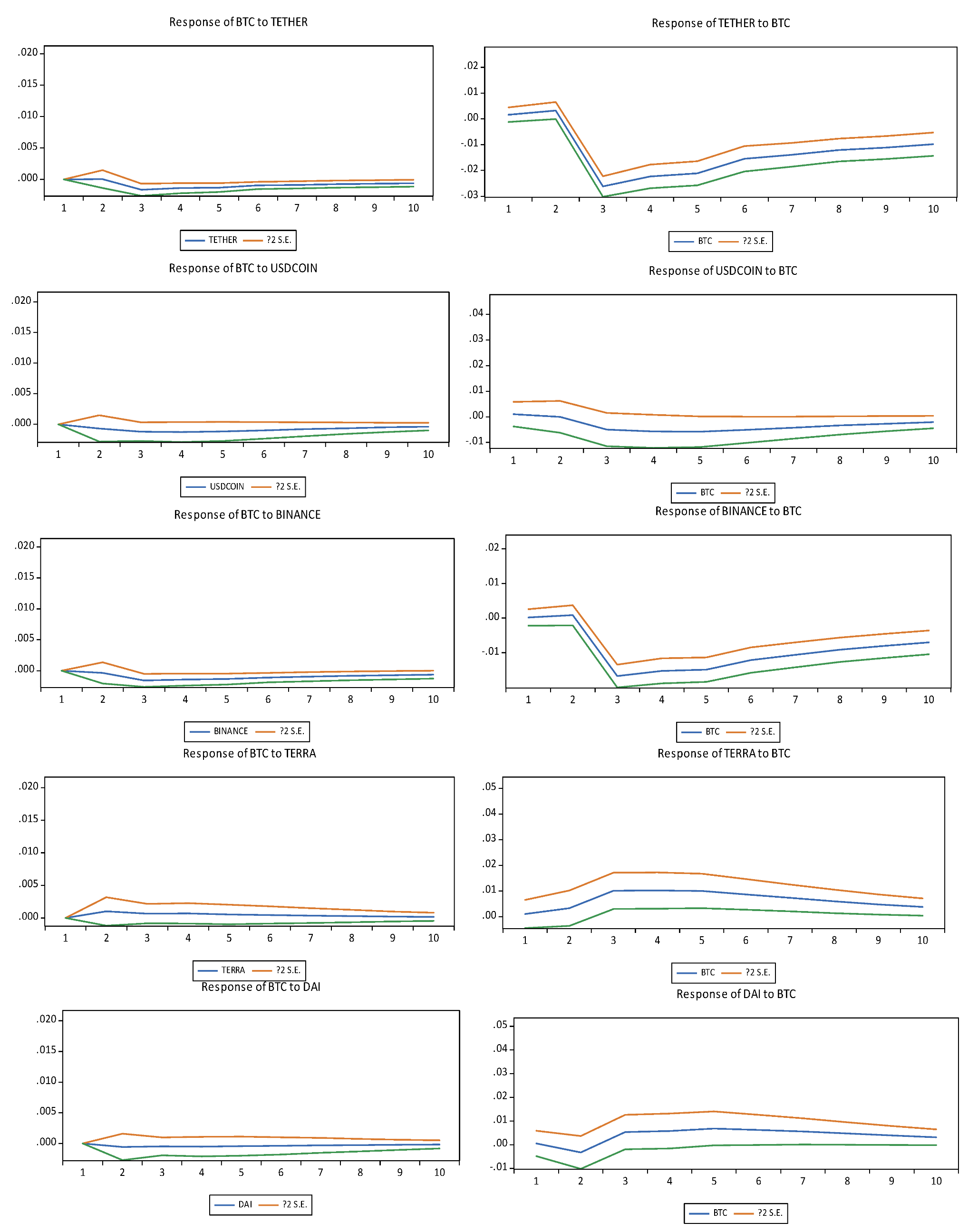
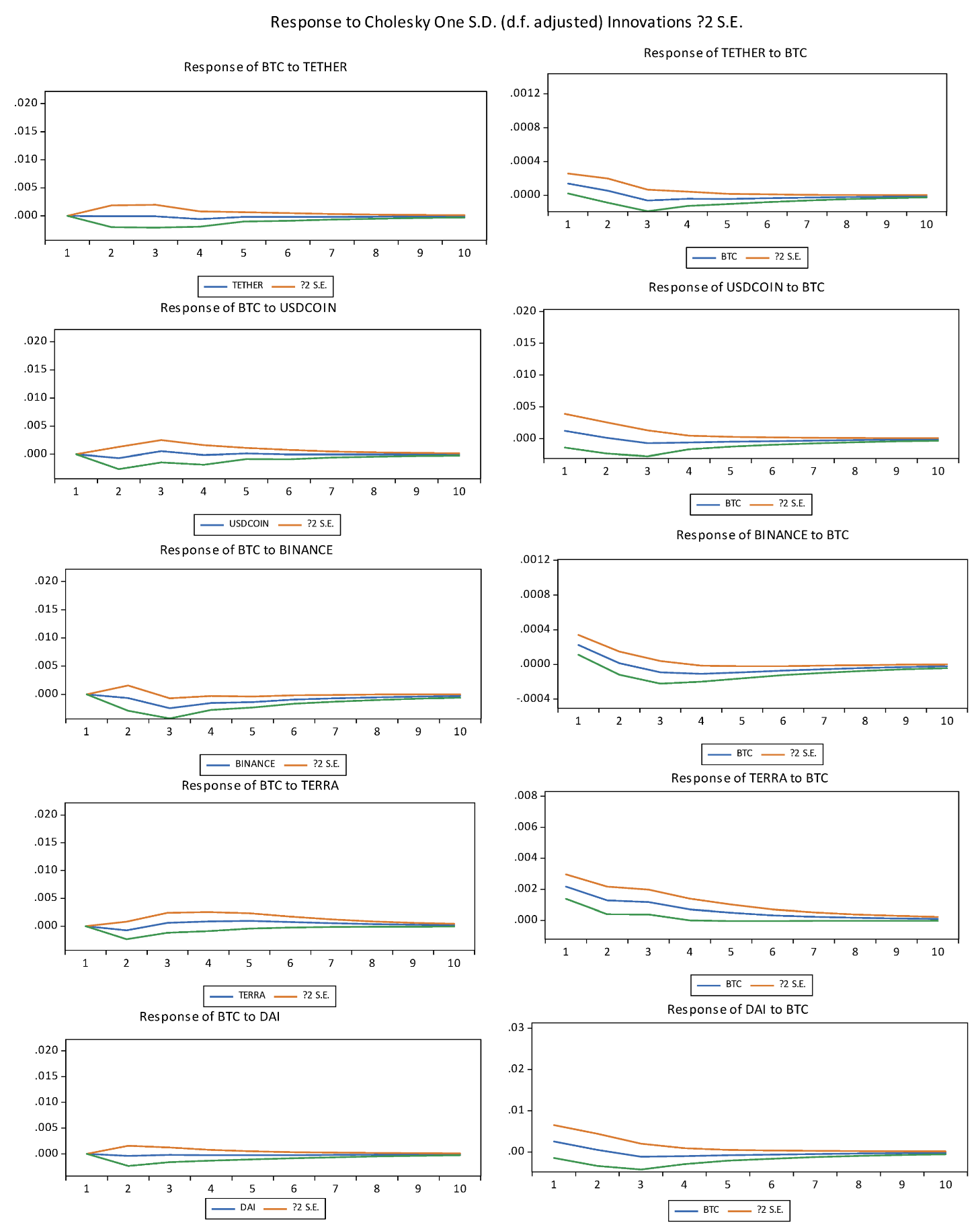
3.4. VAR Granger-Causal Perspective

To examine whether Bitcoin inflates the volatility of stablecoins, one can determine whether it shall be the crucial factor driving volatility in stablecoin markets. To enhance the causal perspective, in this study, the VAR Granger causality test is used in order to examine the stochastic interdependences between the volatility movement of Bitcoin and stablecoins. Following Grobys et al. [11], we employ this approach instantly to the range-based volatilities. Assuming a 6 × 1 vector Yt as Yt = (BTCt, USDTt, USDCt, BUSDt, TUSDt, DAIt)′, we use the vector autoregression (VAR) model as follows:
Yt = c + A1Yt−1 + ⋯ + ApYtp + ut,
where A1, …, Ap represent 6 × 6 parameter matrices, and ut is the residual term distributed as ut ∼ (0, Σu). Where Σu is the corresponding covariance matrix. In addition, c denotes the constant term including a 6 × 1 vector.

4. Empirical Results and Portfolio Implications

4.1. Data Description and Results Analysis

We employ a sample of major cryptocurrencies for Bitcoin (BTC) and the five largest stablecoins on market capitalization included Tether (USDT), USD Coin (USDC), Binance Coin (BUSD), Terra USD (UST), and Dai (DAI) which are retrieved from 1 July 2014 to 15 February 2022. Owing to the data availability, we select this sample period whereby some stablecoins are only available from 23 November 2019. Digital currencies have some distinct features compared to the conventional cryptocurrency and are traded 24/7, the cryptocurrency exchanges occur day and night and are effectively never closed in the global market. The cryptocurrency market data are retrieved from https://www.coinmarketcap.com/price/data (accessed on 25 February 2022) which is the trading platform that is most popular by market participants and provides liquidity for the crypto economy of pricing data for the cryptocurrencies. The cryptocurrency volatilities profile represented in Equations (3)–(5) consists of 8700 observations. As depicted in Table 1, stablecoins market capitalization was at USD 182.5 billion, according to crypto-assets data tracker coinmarketcap.com. Accordingly, the overall market capitalization of stablecoins currently stands at approximately 4% of the total crypto market capitalization. Table 1 also reports the increasing importance of stablecoins in the Fintech ecosystem.

4.2. Results of Range-Based Volatility Approaches

The six panels of Figure 1 depict the time series of the three measures in the range-based volatility of BTC and stablecoins. The top panel exhibits the daily realized volatility of BTC. Perhaps not surprisingly, the measure of the stability of BTC exhibits a highly volatile nature. The second panel plots the daily range-based volatility of Tether implying less volatility; the third panel shows relative stability of the daily range-based volatility of USD Coin; the fourth, and fifth panels depict the historical volatility of Binance USD and Terra USD, respectively. The bottom panel also reports the relative stability of the daily range-based volatility of Dai. Specifically, the range-based volatility with the statistics for the Bitcoin variation corresponds with the analogous findings in the realized volatility of Grobys et al. [11].
As evidenced in the first four moments depicted in Table 2, the visual impressions are conducted by the summary statistics for the mean, variance, skewness, and kurtosis of cryptocurrencies’ volatilities, respectively. Thus, we observe that Bitcoin implies the highest average volatility based on the RS estimator accounting for 3.92%, while the average volatility of stablecoins in the range between 0.36% (PK estimator of USDT) and 1.03% (GK estimator of DAI). Thus, the average volatility of non-stablecoin (BTC) is profoundly larger than the average stablecoin volatilities. This is a crucial stylized empirical fact that we can obtain from each ranged-based volatility series. It also follows that the unconditional distribution of range-based volatility measures (GK, RS estimators) is highly skewed (24.75, 28.40) of stablecoins (USDC), implying evidence of asymmetry. We further suggest that all cryptocurrency volatilities exist widely as heavy-tailed. Indeed, one can measure this statistical phenomenon through the excess kurtosis metric. Table 2 reports that each cryptocurrency’s volatility infers leptokurtic distributions ranging from 15.66 (PK estimator of BTC) to 916.57 (RS estimator of USDC). Finally, we document that the non-stablecoin Bitcoin is much more unstable compared to the stablecoins. Table 2 reports the qualitative features and precise information given in Figure 1. The time series evolution of the calculated cryptocurrency volatilities from their range-based estimators in Equations (3)–(5). In summary, an important stylized empirical fact emerges from Table 2 and Figure 1 and infers that there is a heavy-tail phenomenon in all cryptocurrency volatilities, see also Chen, et al. [31].
To estimate the volatility of various crypto assets, we first employ the range-based volatility approaches, and the results are depicted in Table 2. As stablecoins and digital token markets are in the emerging stage and developing economies, the Fintech savvy in this crypto ecosystem may cause information asymmetry in market participation as their transaction strategy. From the empirical evidence of stablecoins, our finding emphasizes properties common to the argument that the volatility dynamics of large-cap stablecoins can be explained to drive the smaller-cap ones. Thus, stablecoin users can lightly convert the various stablecoins into the other cryptocurrency market.

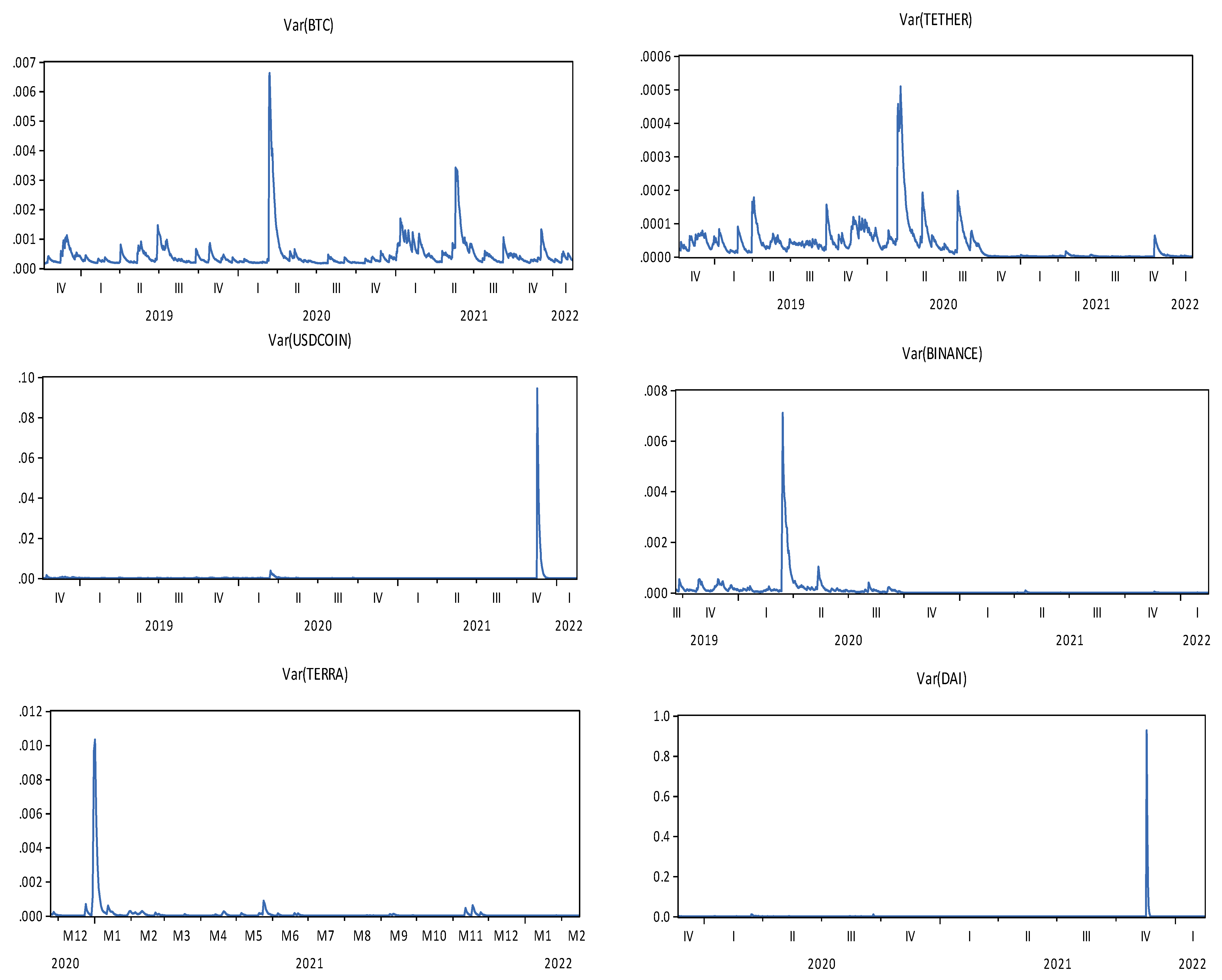
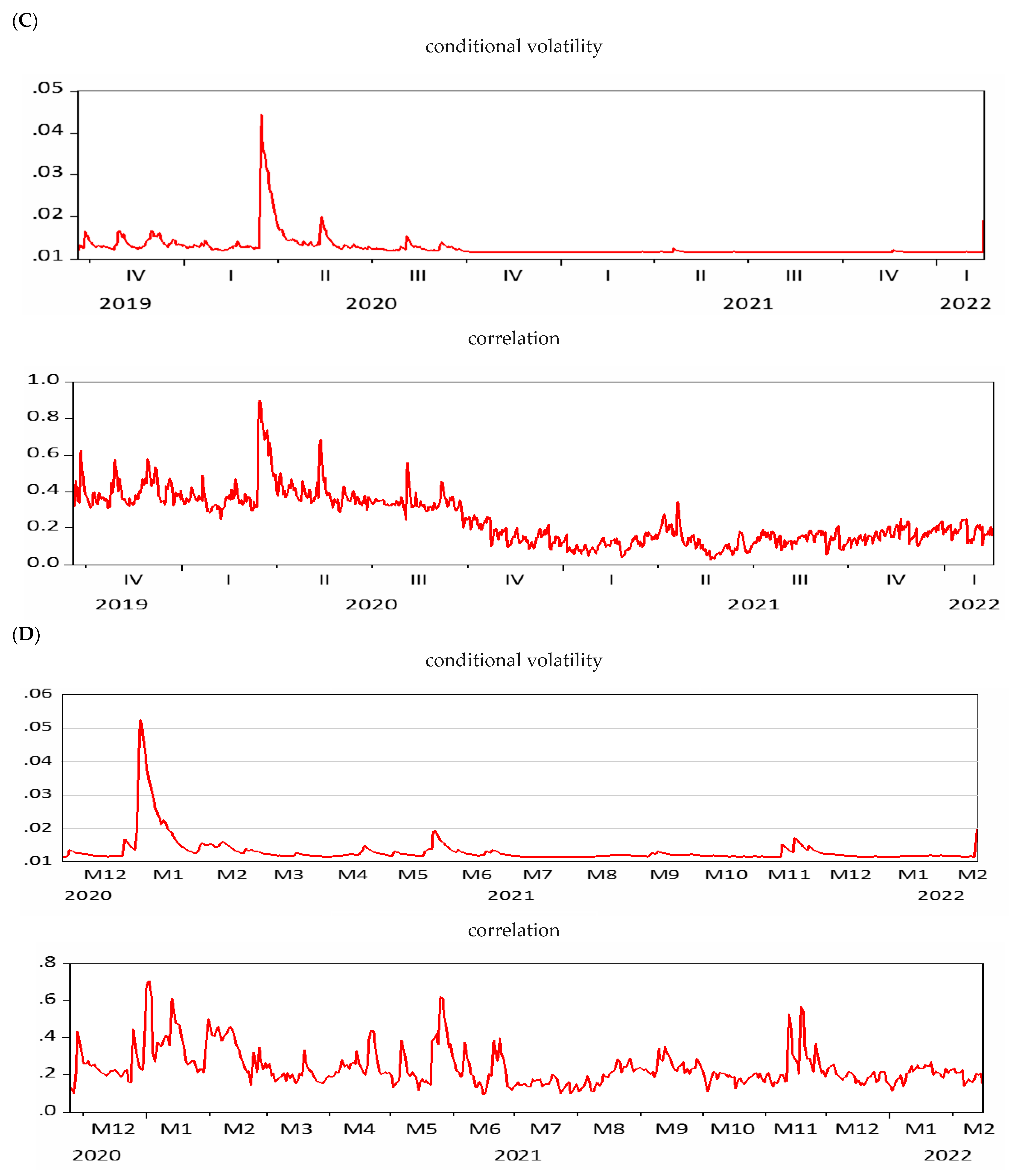
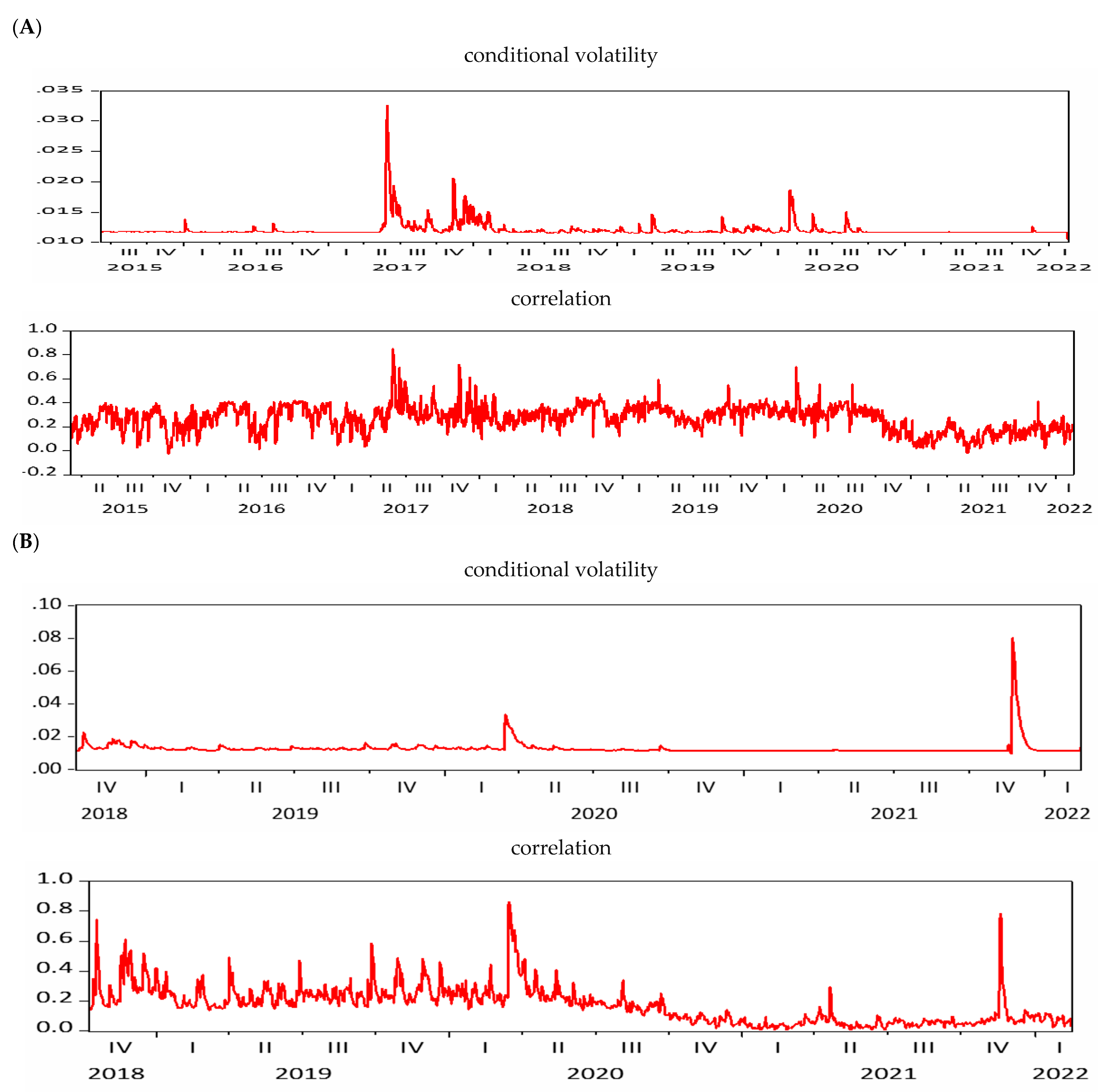
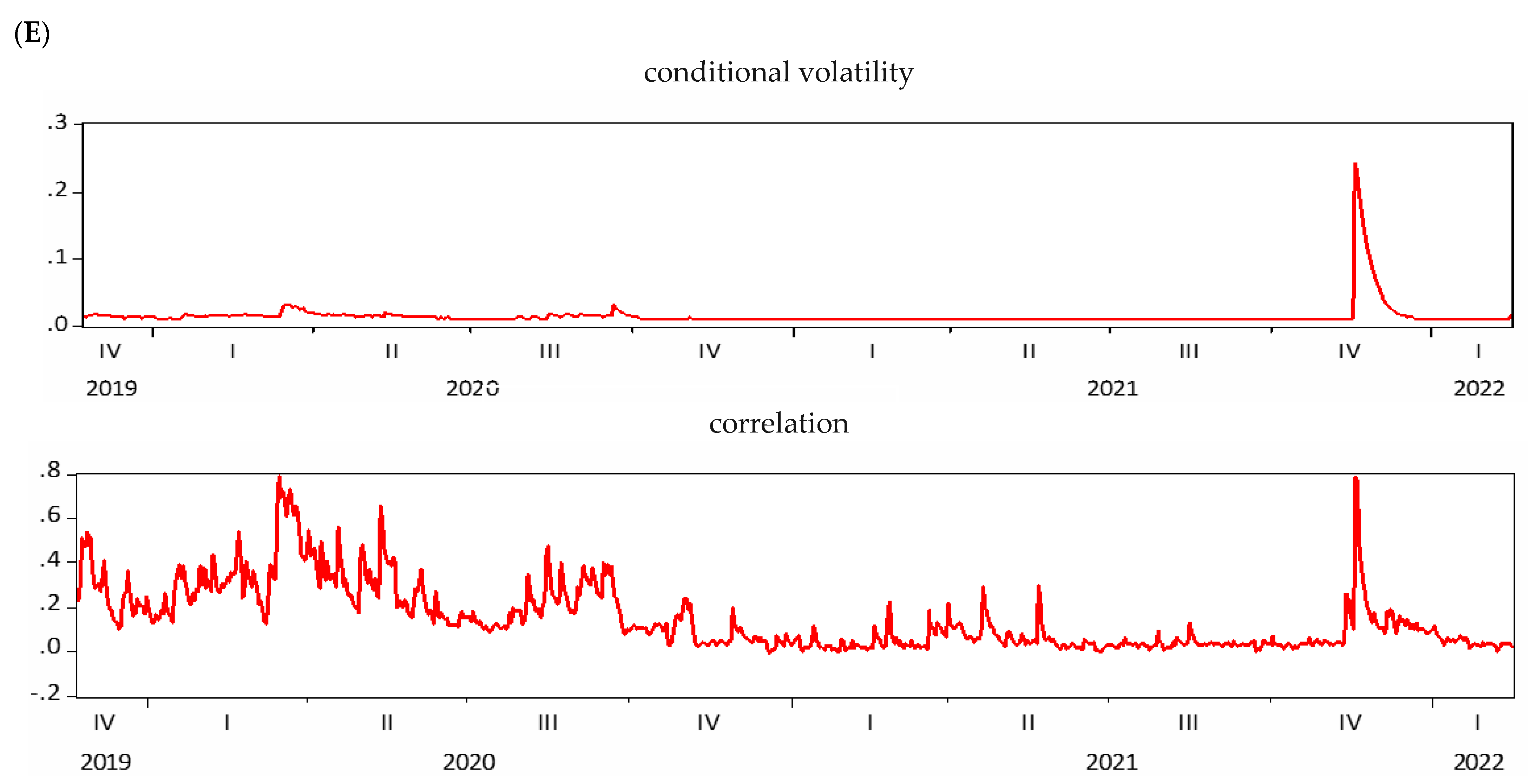
4.3. The BEKK–GARCH Model Results

The BEKK–GARCH model is used on the stationary series to explore both conditional covariance and conditional correlations. Hence, we apply this approach to study the volatility co-movement between Bitcoin and stablecoins. Table 3 reports parameter estimates for the five scenarios via the BEKK–GARCH (1, 1) model.
In this multivariate modeling, ϕ i i = 1, 2, 3, and 5 are statistically insignificant rejecting any relationship in volatility co-movement among the Bitcoin against various stablecoins, except for BTC versus Terra USD ( ϕ 4 ) . Turning out to the findings of the spillover effect in Bitcoin and stablecoin markets, the BEKK–GARCH estimation shows the unidirectional spillovers from the Bitcoin market to the Terra USD market. Overall, the evidence demonstrates that the volatility shocks of the Bitcoin market results and the coefficients are insignificant. Thus, it can be reasonably interpreted that volatility shocks in Bitcoin could not have a significant impact on other stablecoins. The result is in line with the finding of Zięba et al. [32], who argued insignificant shock and volatility spillovers from Bitcoin to other cryptocurrencies.
However, the findings are different from many papers that concentrate on interconnecting that the most important cryptocurrencies (Bitcoin) are manipulated by the stablecoin (Tether), such as Griffin and Shams [6], Hoang and Baur [10] and Grobys [11]. Additionally, as the estimated parameters of ARCH and GARCH coefficients, (i.e., α i j and β i j ), which mainly capture shock dependence and the persistent volatility of the conditional variance equations, and common patterns observed between Bitcoin and stablecoins. Indeed, these coefficients are statistically significant among the various scenarios (in most scenarios). The volatility response to past conditional volatility (ARCH and GARCH terms) is significant for all Bitcoin vs. stablecoin volatility series at the 1% level. Interestingly, a more thorough exploration of the modeling results for stablecoins infer that the serial correlations become insignificant. There is little correlation between the volatility movement of Bitcoin and volatility for the stablecoins. As shown in Figure 2, there are time-varying conditional correlations between Bitcoin against other cryptocurrency’s volatility. Indeed, both BTC Terra and Tether USD are consistently positively associated with correlations varying from +0.01 on the low to nearly +1 on the high. Finally, as depicted in Figure 3, considering the conditional variance in the fitted BEKK–GARCH, the volatilities of stablecoins are considerably more stable than the Bitcoin volatility. Considering the potential of copula functions, we estimate the volatility co-movement between Bitcoin and each stablecoin using a Copula–DCC–GARCH model. As depicted in Table 4, results exhibit that the volatility of prices seems to be more dependent and conditional to past information. As it can be observed, with the exception of joint distribution parameters (dcc a, b) evidenced by the significance of the parameters, imply that the Copula–DCC–GARCH model performs a good fit for cryptocurrencies’ volatility.
To investigate the contemporaneous correlation between Bitcoin and stablecoins, different models are employed compared to the BEKK–GARCH approach. Empirically, in this adoption copula DCC–GARCH model, there are some advantages against other competing models such as GARCH type or BEKK–GARCH models. The reasons for this phenomenon are twofold. First, copulas are briefly described with skewed and leptokurtic distributions as the BTC one (Table 2), which are the real questions to other models. Second, the BEKK–GARCH parameterization exhibits nonlinearity; thus, its parameters are difficult to interpret, for example, see Block et al. [23].
As time-varying volatility has found applications in extensive modeling in financial time series, it especially draws attention to the issues of cryptocurrency markets. Overall, the empirical result when employing the Student-t DCC copula depicts the dynamic dependence between Bitcoin and stablecoins, in response to the structural transformation. The trajectories of the time-varying correlation of each BTC vs. stablecoins pair are plotted in the bottom panel of Figure 4, respectively. To be specific, Figure 4 shows that the dependence between Bitcoin and stablecoins is more volatile, as it varies ranging from a minimum of 0.001 to a maximum of 0.85. Eventually, we report that the dependence parameters are awfully volatile. Regarding each pair of BTC and stablecoins, the relationship BTC–USDT (unconditional correlations: 0.4312) case seems to be more interconnected than that of BTC versus the other cryptocurrency cases.
Figure 1. Results for range-based volatility estimators among Bitcoin and stablecoins markets. Note: The ticker is denoted for Bitcoin (BTC), Tether (USDT), USD Coin (USDC), Binance USD (BUSD), Terra USD (UST), and Dai (DAI).
Axioms 11 00259 g001
Table 2. Descriptive statistics of range-based volatility estimators.
BTCUSDTUSDC
σ ^ P K 2 σ ^ R S 2 σ ^ G K 2 σ ^ P K 2 σ ^ R S 2 σ ^ G K   2 σ ^ P K 2 σ ^ R S 2 σ ^ G K 2
Mean0.0278520.0392450.0266140.0036010.0088800.0078040.0066590.0081990.008770
Median0.0216010.0292240.0200300.0016270.0061150.0037560.0047610.0053160.006336
Maximum0.2939440.5024680.2609570.0854310.1357820.1653810.5133870.8529990.604452
Minimum0.0015090.0022080.000000.000000.000000.000000.000000.000000.00000
Std. Dev.0.0240040.0353890.0244610.0055990.0105790.0110570.0162400.0259620.019211
Skewness2.6295412.8058153.0575254.2887963.8083024.65745825.1882528.4021524.75231
Kurtosis15.6603919.3922618.4852536.5680630.5188346.13120775.5576916.5785756.4662
Jarque-Bera21824.9234860.3132188.31127091.286319.75206145.8306434544283520229149533
Probability0.0000 ***0.0000 ***0.0000 ***0.0000 ***0.0000 ***0.0000 ***0.0000 ***0.0000 ***0.0000 ***
ADF Prob.0.000 ***0.000 ***0.000 ***0.000 ***0.000 ***0.000 ***0.000 ***0.0001 ***0.000 ***
Observations 2787 2541 1227
BUSDUSTDAI
σ ^ P K 2 σ ^ R S 2 σ ^ G K 2 σ ^ P K 2 σ ^ R S 2 σ ^ G K 2 σ ^ P K 2 σ ^ R S 2 σ ^ G K 2
Mean0.0053650.0072540.0066390.0068560.0090210.0081130.0086000.0114590.010367
Median0.0024720.0044550.0032220.0045130.0060330.0053690.0038290.0057280.004364
Maximum0.1165710.1429810.1478350.1393730.2074740.1277930.7840880.9231661.294481
Minimum0.000008.28E-050.0000000.0000000.0007610.0002310.000008.29E-050.000173
Std. Dev.0.0078480.0095220.0096520.0100940.0146270.0101720.0298950.0355590.048217
Skewness5.8311866.1717795.8319637.9079339.5804325.76168322.1123521.3838423.87537
Kurtosis65.2650070.7478165.8385289.76793118.621354.09976560.7605535.2409622.9322
J.-B.147141.2173878.1149773.3145204.5256394.851220.8410656834970560013160374
Probability0.0000 ***0.0000 ***0.0000 ***0.0000 ***0.0000 ***0.0000 ***0.0000 ***0.0000 ***0.0000 ***
ADF Prob. 0.000 ***0.000 ***0.000 ***0.000 ***0.000 ***0.000 ***0.000 ***0.001 ***0.000 ***
Observations 880 448 817
*** represents statistical significance at the 1% level; The volatilities is measured for Bitcoin (BTC), Tether (USDT), USD Coin (USDC), Binance USD (BUSD), Terra USD (UST), and Dai (DAI); Range-based volatility estimators are computed from equation as Equations (3)–(5); J.-B. denotes Jarque–Bera statistic test.

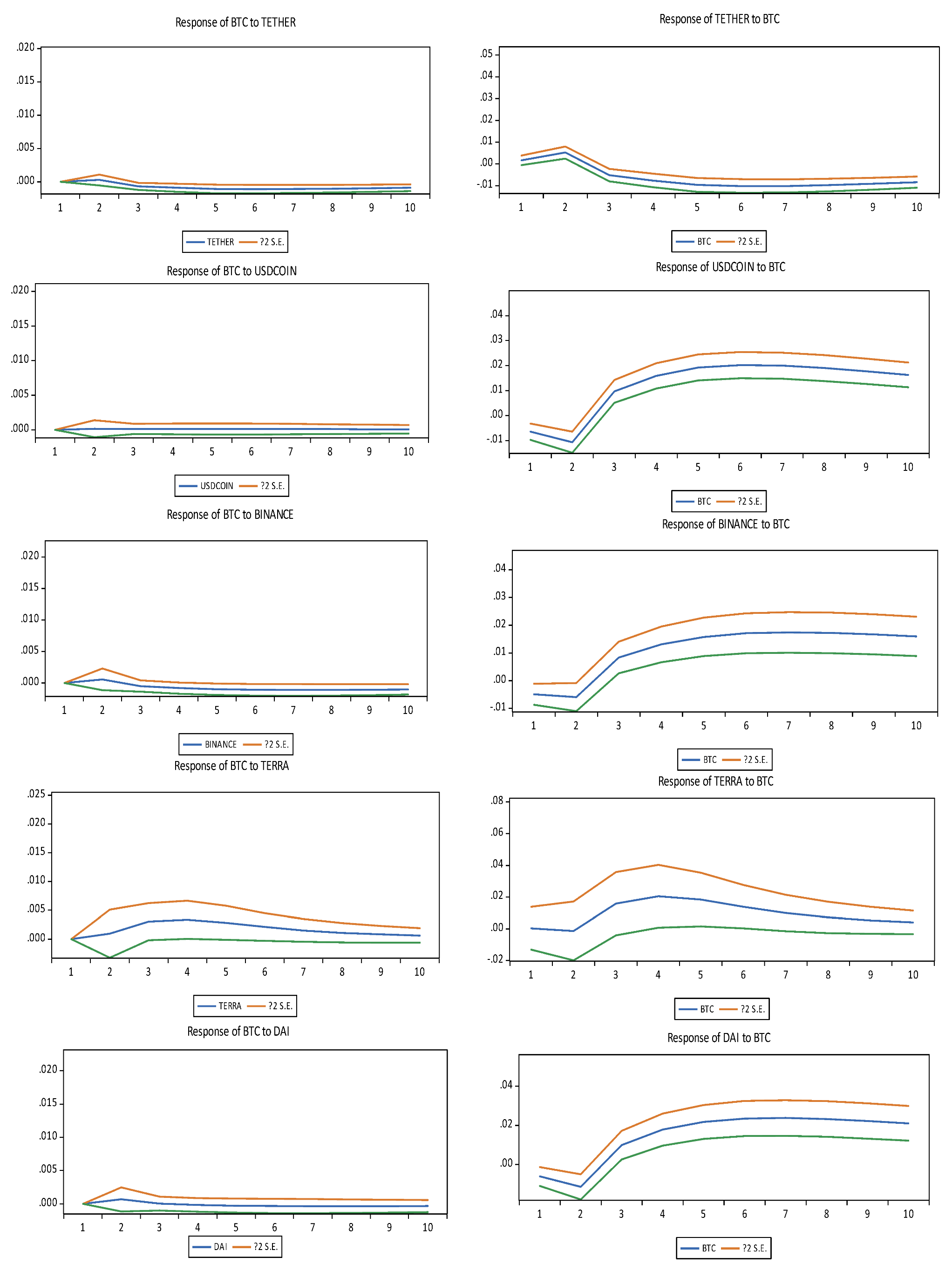
4.4. VAR Granger Causality Test Results

To examine the volatility fluctuations across the Bitcoin and stablecoin markets, we conduct a Granger causality test based on the VAR model to capture the information flow of these cryptocurrencies that are connected to each other. The evidence of various causal relationships is shown in Table 5. Unsurprisingly, there is no directional causality transmission from the BTC market to the five stablecoin markets (Tether, USD Coin, Binance Coin, Terra, and Dai), supporting no volatility spillover from the BTC prices to the stablecoin prices. Unsurprisingly, the Granger causality among the BTC, Tether, USD Coin, Binance Coin, Terra, and Dai markets is less pronounced. There is perhaps mean reversion in equilibrium stablecoin prices under the market correction mechanism even though parity deviations of the major stablecoin are strongly affected by Bitcoin volatility. However, our results suggest that the high volatility of BTC fails to Granger-cause stablecoin price changes at the 5% significance level. In addition, the stablecoin price changes fail to Granger-cause high volatility of BTC at the 10% significance level. As depicted in Table 5, the Granger causality test exhibits that changes in its volatility do not Granger-cause changes on bidirectional linkages that are disclosed between the volatility in the BTC and stablecoin markets. The finding is analogous to Wei (2018) [7], who found that Tether issuances did not Granger-cause Bitcoin returns, and Tether manipulation lead to the 2017 Bitcoin rally. However, our findings contradict Katsiampa et al. [33].
Table 3. The results of the bivariate BEKK-GARCH model parameter estimates.
BTC-USDTBTC-USDCBTC-BUSDBTC-USTBTC-DAI
ParameterCoeff.p-ValueCoeff.p-ValueCoeff.p-ValueCoeff.p-ValueCoeff.p-Value
Conditionalmean
μ0.000730.000 ***0.001460.000 ***0.001040.000 ***0.003260.000 ***0.001680.000 ***
ϕi0.000140.9396−0.000470.0173 **−0.002640.11220.023620.0011 ***−0.000190.5559
u
Conditional variance
c111.98 × 10−50.000 ***1.89 × 10−50.0001 ***1.46 × 10−50.002 ***0.000120.18540.01630.000 ***
c12−1.86 × 10−70.2196−4.48 × 10−70.4467−1.397 × 10−70.52598.15 × 10−60.15150.27520.000 ***
c225.65 × 10−80.000 ***4.767 × 10−70.000 ***7.76 × 10−80.004 ***9.75 × 10−60.08011.12 × 10−60.000 ***
α110.06070.000 ***0.0830.000 ***0.03910.000 ***0.133780.0038 ***0.27380.000 ***
α120.09480.000 ***0.269140.000 ***0.11970.000 ***0.257310.123921.23160.000 ***
α220.14820.000 ***0.871040.000 ***0.36730.000 ***0.494850.0009 ***0.97140.10523
β110.90310.000 ***0.874210.000 ***0.91040.000 ***0.819460.000 ***0.9093970.10066
β120.89490.000 ***0.684560.000 ***0.82420.000 ***0.663680.000 ***0.8749620.06280
β220.88670.000 ***0.536070.000 ***0.74620.000 ***0.537560.000 ***0.59470.000 ***
Durbin-Watson stat. 0.8115 1.3655 1.16120 1.5853 1.5647
Schwarz criterion −22.921 −13.364 −14.113 −13.439 −13.282
Log likelihood 14129.27 8239.93 6250.68 3046.99 5459.43
Q2 (h) 17.052 12.028 187.953 11.478 9.221
(0.5195) (0.444) (0.000 +) (0.0217) (0.684)
Notes: *** and ** report the 1% and 5% at significance levels, respectively; Q 2 ( h ) is Q-stat. on the standardized squared residuals and + reports the rejection of the null hypotheses of no residual autocorrelations up to lag h at the 10% significance level. Parentheses is p-value; In Equation (7), μ = ( μ 1 ,   , μ i ) is a vector matrix of the conditional mean term of Bitcoin and other stablecoins markets, ϕ i i = 1, 2, 3, 4, and 5 indicate the estimated coefficients for BTC-USDT, BTC-USDC, BTC-BUSD, BTC-UST, and BTC-DAI, respectively.
Table 4. The results of the Copula -DCC-GARCH model parameter estimates.
BTC-USDTBTC-USDCBTC-BUSDBTC-USTBTC-DAI
ParameterCoeff.p-Value Coeff.p-ValueCoeff.p-ValueCoeff.p-ValueCoeff.p-Value
a0.00360.0000 ***0.00670.0000 ***0.00540.0000 ***0.00490.0000 ***0.00860.0000 ***
b0.40790.0050 ***0.13530.0000 ***0.29670.0918 *0.25380.0011 ***0.07870.0000 ***
c0.0018820.0000 ***0.0014790.0000 ***0.0005040.0000 ***0.0005690.0001 ***0.0002710.0000 ***
α0.8783330.0000 ***0.6864320.0000 ***0.8773980.0000 ***0.5745200.0000 ***0.8203750.0000 ***
β0.0905300.0000 ***0.2564790.0000 ***0.1068640.0000 ***0.3997820.0021 ***0.2756930.0000 ***
Log likelihood 12861.02 5128.84 4547.35 2138.93 3627.32
Unconditional correlations 0.4312 0.1331 0.3094 0.2664 0.0638
Notes: *** and * denote 1% and 10% at significance levels, respectively; Parameters a, b denotes the estimated Joint (DCC) parameters; The volatility linkages across Bitcoin and five major cryptocurrency markets are examined adopting the copula-GARCH models estimated in two stages. In the first stage, the GARCH model is used to time series of range-based volatility via EViews 11, while in the second stage the estimation of conditional copula models is fitted by Excel.
Figure 2. Conditional correlations between the Bitcoin and stablecoins markets (VAR-BEEK-GARCH model). Notes: Bitcoin–stablecoins correlation via the VAR–BEKK–GARCH model.
Axioms 11 00259 g002
Figure 3. Conditional variance for the Bitcoin and top five stablecoins based on the VAR–BEEK–GARCH model.
Axioms 11 00259 g003

4.5. Robustness Test

For a robustness check, the impulse responses are summarized in Figure 5 and provide whether they diminish over time, and how. The Figure 5 exhibits ten charts. In the first standard chart, the VAR system features the conditional covariances of group 1 (BTC-Tether) cryptocurrencies. We see that in the short-run, dynamics emerge, and Bitcoin does not significantly drive the volatilities of stablecoins, nor is it affected by stablecoins. The result is in line with Kristoufek [34]. For instance, a 0.25-point impulse to the recession probability (R) creates a 0.2 percent sputter in the covariance between the volatilities (price changes) of Bitcoin and Tether after two periods. The responses of the Bitcoin and stablecoins pair are similar in direction but the relatively slight magnitude. The responses to the recession impulse occur with three lags. To ensure the robustness of the model, we detect the impulse response functions (IRFs) of each cryptocurrency over the entire period in the preceding content. Robustness analysis is further introduced and the entire period is divided into two subperiods. Bitcoin surpassing USD 60,000 in its first record high on 13 March 2021 is regarded as the breakpoint in volatility regimes. On the basis of the breakpoints for each cryptocurrency, the sample period is divided into two subperiods, which correspond to the before/after breakpoint (13 March 2021), respectively. Figure 6 depicts breakpoints in the IRFs of six cryptocurrencies over subperiod 1 from 6 March 2015 to 13 March 2021 (corresponding to the sample period 2 post-13 March 2021 depicted in Figure 7). Figure 6 and Figure 7 report the accumulated IRFs from estimating VAR (2) processes, (i.e., two lags) where %∆Bitcoin and %∆ stablecoins are treated endogenously. The response of %∆Bitcoin is exhibited in response to a two standard deviation exogenous shock to %∆ stablecoins. The solid line displays the IRFs while the dotted lines denote the upper and lower bound given two standard deviation. In summary, further robustness analysis is divided into two main groups and the IRFs of each cryptocurrency are examined to find consistent results over the two subperiods compared to the entire period in the preceding content.
Figure 4. Conditional volatility and correlation between Bitcoin and stablecoins (Copula–DCC–GARCH model). (A) Bitcoin vs. Tether. (B) Bitcoin vs. USD Coin. (C) Bitcoin vs. Binance USD. (D) Bitcoin vs. Terra USD. (E) Bitcoin vs. Dai. Notes: As plotted in Figure 4 the upper, and bottom panels denote conditional volatility and correlation series, respectively.
Axioms 11 00259 g004aAxioms 11 00259 g004bAxioms 11 00259 g004c
Table 5. VAR Granger causality tests for BTC and stablecoins.
Dependent Variable: BTC
ExcludedChi-sqdfProb.
USDT0.82253420.6628
USDC0.14583620.9297
BUSD7.26124820.0265
UST1.53398120.4644
DAI0.20451420.9028
All10.78848100.3742
Dependent Variable: USDT
ExcludedChi-sqdfProb.
BTC4.42912920.1092
USDC10.6106420.0050 *
BUSD14.1221120.0009 *
UST10.7812720.0046 *
DAI7.87843520.0195
All68.78196100.0000
Dependent Variable: USDC
ExcludedChi-sqdfProb.
BTC0.71403120.6998
USDT1.17164820.5566
BUSD1.81437720.4037
UST0.14216320.9314
DAI0.54503620.7615
All3.698988100.9599
Dependent Variable: BUSD
ExcludedChi-sqdfProb.
BTC6.12038720.0469
USDT2.27169320.3212
USDC4.76113020.0925
UST1.80081220.4064
DAI3.50903020.1730
Note: (*) reports rejection of the null hypothesis (no Granger causality) at the 1% significance level.
Figure 5. VAR impulse responses of the Bitcoin and stablecoins stability (entire period).
Axioms 11 00259 g005
Figure 6. VAR impulse responses of the Bitcoin to stablecoins by subperiod 1 (pre-13 March 2021).
Axioms 11 00259 g006
Figure 7. VAR impulse responses of the Bitcoin to stablecoins by subperiod 2 (post-13 March 2021).
Axioms 11 00259 g007

5. Conclusions

In this paper, we investigate the range-based volatility of stablecoins and conduct a new specification of the BEKK model to examine their potential stochastic interconnection with Bitcoin volatility. Our results provide fresh empirical insights and arguments that Bitcoin volatility exhibits relatively well-behaved statistical distributions due to a theoretical variance convergence, (e.g., Grobys et al., 2021 [11]). Although the presence of temporary deviation, the stablecoins’ volatilities are considerably more stable and contemporaneously respond to Bitcoin volatility under the reversion mechanism. In addition, there are no bidirectional Granger causal interactions between lagged Bitcoin volatility and stablecoins’ volatilities. Consequently, we suggest that excessive Bitcoin volatility is not a crucial component that is driving the stablecoins’ volatility. Our study provided evidence for the absence of volatility spillover linkage across the largest cryptocurrency BTC and major stablecoins. Crucially, Bitcoin could coexist and interconnect with stablecoins.
In summary, our study sheds light on exploring the volatility movements of Bitcoin and the interrelation with stablecoins’ volatility. Our results infer that Bitcoin volatility exhibits more erratically in the statistical property. Moreover, the volatilities of stablecoins exist with more stability. Bitcoin could co-stabilize with stablecoins.
We have also presented an empirical application to the five most heavy transactions in the stablecoins markets, namely Tether, USD Coin, Binance, Terra, and Dai. In this study, we find no evidence to show the destabilizing effects of Bitcoin and stablecoins. Our empirical results, using the Granger causality test based on the specification of the VAR model, support the absence of volatility spillovers across the Bitcoin and stablecoin markets. We also infer that parity deviations of the major stablecoin Tether have been slightly affected by Bitcoin volatility. The result is analogous to Wei (2018) [7] who investigated the largest stablecoin Tether and its impact on Bitcoin and documented the impossible price manipulation in Bitcoin.
Finally, USD-pegged stablecoins are described as a ‘crypto finance ecosystem’ specifically decentralized finance (DeFi) that is responsible for fueling demand for stablecoins that has led to rapid growth. Regarding volatility behavior for Bitcoin and the top five stablecoins, low and high prices express crucial information about the volatility movement of crypto assets. From a volatility trading strategies perspective, the study provides policy implications for crypto investors and portfolio managers to hedge the crypto asset’s risk by adding stablecoin. We expect that the findings from this research can be useful to provide strategic insights for crypto investors and portfolio managers to recognize the stablecoins’ precise guiding mechanism in cryptocurrency markets. Empirically, as we report, some stablecoins such as Tether and Terra USD (UST) have lost their peg on two occasions during the global COVID-19 crisis of March 2020. Accordingly, crypto investors may be cautious with stablecoin adoption in their portfolios to diversify the portfolios’ risk from Bitcoin volatility to the greatest possible extent for value protection.
As shown in the above results, the major range-based volatility measures provide consistent results; however, the efficiency of these estimators and the role of stablecoins’ safe haven are not discussed in this study and will be left to further work.

Author Contributions

Conceptualization, K.-S.C.; methodology, K.-S.C.; software, K.-S.C.; investigation, K.-S.C.; resources, S.-H.C.; writing—review and editing, S.-H.C. All authors have read and agreed to the published version of the manuscript.

Funding

This research received no external funding.

Institutional Review Board Statement

Not applicable.

Informed Consent Statement

Not applicable.

Data Availability Statement

Not applicable.

Acknowledgments

The authors sincerely thank the editors and the three anonymous reviewers for their insightful comments and constructive suggestions that enrich and improve substantially our paper to a higher level. Of course, any errors are the authors’ responsibility.

Conflicts of Interest

The authors declare no conflict of interest.

References

  1. Sidorenko, E.L. Stablecoin as a new financial instrument. In Digital Age: Chances, Challenges and Future; Ashmarina, S., Vochozka, M., Mantulenko, V., Eds.; Springer International Publishing: Cham, Switzerland, 2020; pp. 54–96. [Google Scholar]
  2. Wang, G.J.; Ma, X.Y.; Wu, H.Y. Are stablecoins truly diversifiers, hedges, or safe havens against traditional cryptocurrencies as their name suggests? Res. Int. Bus. Financ. 2020, 54, 101225. [Google Scholar] [CrossRef]
  3. Xie, Y.; Kang, S.B.; Zhao, J. Are stablecoins safe havens for traditional cryptocurrencies? An empirical study during the COVID-19 pandemic. Appl. Financ. Lett. 2021, 10, 2–9. [Google Scholar] [CrossRef]
  4. Ito, K.; Mita, M.; Ohsawa, S.; Tanaka, H. What is Stablecoin? A Survey on Its Mechanism and Potential as Decentralized Payment Systems. Int. J. Serv. Knowl. Manag. 2020, 4, 71–86. [Google Scholar] [CrossRef]
  5. Lyons, R.K.; Viswanath-Natraj, G. What Keeps Stablecoins Stable? (No. w27136); National Bureau of Economic Research: Cambridge, MA, USA, 2020. [Google Scholar]
  6. Griffin, J.M.; Shams, A. Is Bitcoin really untethered? J. Financ. 2020, 75, 1913–1964. [Google Scholar] [CrossRef]
  7. Wei, W.C. The impact of Tether grants on Bitcoin. Econ. Lett. 2018, 171, 19–22. [Google Scholar] [CrossRef]
  8. Kristoufek, L. On the role of stablecoins in the cryptoassets pricing dynamics. Financ. Innov. 2022, 8, 37. [Google Scholar] [CrossRef]
  9. Lyons, R.K.; Viswanath-Natraj, G. Stable Coins Don’t Inflate Crypto Markets VOX CEPR Policy Portal. 2020. Available online: https://voxeu.org/article/stable-coins-dont-inflate-crypto-markets (accessed on 5 December 2020).
  10. Hoang, L.T.; Baur, D.G. How stable are stablecoins? Eur. J. Financ. 2021. [Google Scholar] [CrossRef]
  11. Grobys, K.; Junttila, J.; Kolari James, W.; Sapkota, N. On the stability of stablecoins. J. Empir. Financ. 2021, 64, 207–223. [Google Scholar] [CrossRef]
  12. Baba, Y.; Engle, R.F.; Kraft, D.F.; Kroner, K.F. Multivariate Simultaneous Generalized ARCH (Working Paper); Department of Economics, University of California at San Diego: San Diego, CA, USA, 1990. [Google Scholar]
  13. Engle, R.F.; Kroner, K.F. Multivariate simultaneous generalized ARCH. Econom. Theory 1995, 11, 122–150. [Google Scholar] [CrossRef]
  14. Fiszeder, P. Low and high prices can improve covariance forecasts: The evidence based on currency rates. J. Forecast. 2018, 37, 641–649. [Google Scholar] [CrossRef]
  15. Tan, S.K.; Chan, J.S.K.; Ng, K.H. On the speculative nature of cryptocurrencies: A study on Garman and Klass volatility measure. Financ. Res. Lett. 2020, 32, 101075. [Google Scholar] [CrossRef]
  16. Brandt, M.W.; Diebold, F.X. A No-Arbitrage Approach to Range-Based Estimation of Return Covariances and Correlations. J. Bus. 2006, 79, 61–74. [Google Scholar] [CrossRef]
  17. Li, H.; Hong, Y. Financial volatility forecasting with range-based autoregressive volatility model. Financ. Res. Lett. 2011, 8, 69–76. [Google Scholar] [CrossRef]
  18. Fiszeder, P.; Fałdziński, M.; Molnár, P. Range-based DCC models for covariance and value-at-risk forecasting. J. Empir. Financ. 2019, 54, 58–76. [Google Scholar] [CrossRef]
  19. Molnár, P. High-low range in GARCH models of stock return volatility. Appl. Econ. 2016, 48, 4977–4991. [Google Scholar] [CrossRef]
  20. Jacob, J. Estimation and forecasting of stock volatility with range-based estimators. J. Futures Mark. 2008, 28, 561–581. [Google Scholar] [CrossRef]
  21. Todorova, N.; Husmann, S. A comparative study of range-based stock return volatility estimators for the German market. J. Futures Mark. 2012, 32, 560–586. [Google Scholar] [CrossRef]
  22. Bauwens, L.; Hafner, C.M.; Laurent, S. Handbook of Volatility Models and Their Applications; Wiley: Hoboken, NJ, USA, 2012. [Google Scholar]
  23. Block, A.S.; Righi, M.B.; Schlender, S.G.; Coronel, D.A. Investigating dynamic correlation between crude oil and fuels in non-linear framework: The financial and economic role of structural breaks. Energy Econ. 2015, 49, 23–32. [Google Scholar] [CrossRef]
  24. Mensi, W.; Hammoudeh, S.; Nguyen, D.K.; Yoon, S.M. Dynamic spillovers among major energy and cereal commodity prices. Energy Econ. 2014, 43, 225–243. [Google Scholar] [CrossRef]
  25. Parkinson, M. The extreme value method for estimating the variance of the rate of return. J. Bus. 1995, 53, 61–65. [Google Scholar] [CrossRef]
  26. Garman, M.B.; Klass, M.J. On the estimation of security price volatilities from historical data. J. Bus. 1980, 53, 67–78. [Google Scholar] [CrossRef]
  27. Rogers LC, G.; Satchell, S.E. Estimating variance from high, low and closing prices. Ann. Appl. Probab. 1991, 1, 504–512. [Google Scholar] [CrossRef]
  28. Katsiampa, P. Volatility co-movement between Bitcoin and Ether. Financ. Res. Lett. 2019, 30, 221–227. [Google Scholar] [CrossRef] [Green Version]
  29. Engle, R.F. Dynamic conditional correlation—A simple class of multivariate GARCH models. J. Bus. Econ. Stat. 2002, 20, 339–350. [Google Scholar] [CrossRef]
  30. Righi, M.; Ceretta, P. Global risk evolution and diversification: A Copula- DCC- GARCH model approach. Rev. Bras. Financ. 2012, 10, 529–550. [Google Scholar] [CrossRef]
  31. Chen, K.S.; Huang, Y.C. Detecting Jump Risk and Jump-Diffusion Model for Bitcoin Options Pricing and Hedging. Mathematics 2021, 9, 2567. [Google Scholar] [CrossRef]
  32. Zięba, D.; Kokoszczyński, R.; Śledziewska, K. Shock transmission in the cryptocurrency market. Is Bitcoin the most influential? Int. Rev. Financ. Anal. 2019, 64, 102–125. [Google Scholar] [CrossRef]
  33. Katsiampa, P.; Corbet, S.; Lucey, B. Volatility spillover effects in leading cryptocurrencies: A BEKK-MGARCH analysis. Financ. Res. Lett. 2019, 29, 68–74. [Google Scholar] [CrossRef] [Green Version]
  34. Kristoufek, L. Tethered, or Untethered? On the interplay between stablecoins and major cryptoassets. Financ. Res. Lett. 2021, 43, 101991. [Google Scholar] [CrossRef]
Table 1. Characteristics and market capitalization of Bitcoin and stablecoins.
# RankNameTickerCoinmarkPrice24 h %7 d %Market Cap
1BitcoinBTC Axioms 11 00259 i001$44,575.29.65%5.45%$845,117,683,687
3TetherUSDT Axioms 11 00259 i002$1.000.01%0.01%$78,515,395,493
5USD CoinUSDC Axioms 11 00259 i003$0.99980.06%0.03%$52,536,446,749
13Binance USDBUSD Axioms 11 00259 i004$1.000.06%0.00%$17,805,102,313
17Terra USDUST Axioms 11 00259 i005$0.99990.08%0.21%$11,619,278,219
19DaiDAI Axioms 11 00259 i006$0.99930.05%0.03%$10,373,205,726
Notes: Daily data are collected for Bitcoin (BTC), Tether (USDT), USD Coin (USDC), Binance USD (BUSD), Terra USD (UST), and Dai (DAI) from https://coinmarketcap.com/view/stablecoin/ (accessed on 25 February 2022). Top cryptoassets by market cap, rank, price volatility, and available time period for each cryptocurrency as of 15 February 2022. Where 24% and 7 d% denote cryptocurrency i’s corresponding daily and weekly volatility, respectively.
Publisher’s Note: MDPI stays neutral with regard to jurisdictional claims in published maps and institutional affiliations.

