Abstract
This study analyzes whether Bitcoin, gold, oil, and stock have the ability to hedge against inflation in high cryptocurrency adoption countries in the periods from January 2010 to March 2021. It is hypothesized that the assets behave differently and thereby respond differently to inflation in different market conditions. Therefore, we employ the Markov Switching Vector Autoregressive to examine these assets’ hedging ability against inflation in both stable and turbulent market regimes. Our main findings are threefold: We show that there exists a structural change and nonlinear relationship between the returns of hedging assets and inflation. Second, all assets can hedge against inflation more effectively in the short run than in the long run. We find that the inflation hedging ability of these assets are weak in the long run for both market regimes. We also find some evidence that the rigidity between the assets and inflation is relatively high in the stable regime. Third, according to the impulse response analysis, we also find that the responses of assets to inflation shock are heterogeneous across two market regimes.
1. Introduction
The average rate of annual global inflation from 1981 to 2020 was 5.4% (World Bank data, 2020). In 2020, the global inflation rate was 1.94%. However, the inflation rate varied significantly across countries, ranging from −2.7% in Qatar to 2360% in Venezuela (See Figure 1). The causes of different levels of inflation are complex. Ref. [1] summarized that inflation differentials were due to interactions among heterogeneity in structures, shocks from both supply and demand sides, as well as monetary policies. Inflation is an important investment risk as it decreases the real value of assets and returns on investment. Therefore, it is imperative for investors to develop strategies to reduce the inflation risk. A method to hedge for the inflation risk is to include assets that value increase (and decrease) with inflation in the investment portfolio [2].
Theoretically, the increase in inflation will lead investors to seek a hedging asset against the decline in the value of money (reducing purchasing power and the standard of living) resulting in a higher demand for the hedging assets. Thus, knowledge regarding future inflation will enable investors to gain excess revenues by investing in hedging assets. We can say that the price of hedging assets may act as a leading indicator of inflation, making them an instrument for hedging against future inflation [3].
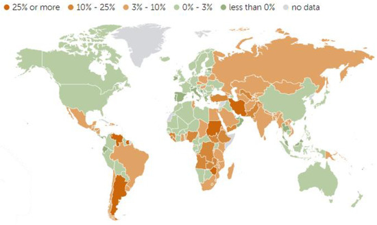
Figure 1.
Inflation in 2020. Source: IMF (2020).
In the literature, there is empirical evidence that the inflation hedging assets could be time varying and may function as a hedge against inflation only in specific market states [4,5]. While the nonlinear relationship between some financial assets and inflation has already been considered, most studies on inflation hedging were limited to the United States and other OEDC countries [6,7]. In addition, studies that performed comparative studies across countries did not include different types of hedging assets such as Bitcoin as a potential hedging tool. As the inflation situation differs across countries, investors in different countries may need different assets to hedge against inflation. This study, therefore, complements the extant literature on the inflation hedging properties of Bitcoin and three other traditional assets, namely gold, oil, and stock markets of the top ten countries with the highest cryptocurrency adoption. Moreover, although some studies have already investigated a link between inflation and Bitcoin [8,9], the nonlinear linkage has not been tested empirically to our knowledge. Hence, this study adopts Markov Switching Vector Autoregressive Regression (MS-VAR) to examine whether Bitcoin and other traditional inflation hedging assets can be used to hedge against inflation in ten countries with the highest rate of cryptocurrency adoption. More precisely, our study can examine the time and place where Bitcoin, gold, oil, and stock act as inflation hedges.
The rest of the paper is organized as follows: Section 2 presents the literature review. Section 3 presents the theoretical framework and methodology used in this study. Section 4 presents the data used in this work. Section 5 reports the empirical results and Section 6 presents the conclusion and discussion.
2. Literature Review
2.1. Inflation Hedge Testing
To examine the inflation hedging ability of gold, oil, Bitcoin, and stock indices, we need to understand the definition of this strategy. The explanation and the examination of the hedge against inflation are usually referred to as the Fisher Theory [10], which states that the expected interest rate should move in the same direction as expected inflation to mitigate the effects of inflation. According to Bodie [11], there are three properties of the inflation-hedging ability of an asset. Firstly, an asset can be viewed as an inflation hedge if the return of the asset should be at least equal to the inflation rate. Secondly, it is an asset that reduces the variance or uncertainty of the future return of another asset. Finally, the last definition, which has been used in almost all empirical studies of inflation hedging, stated that an asset could be viewed as an inflation hedge if inflation and asset return have a positive correlation. Specifically, Fama and Schwert [12] revealed that if the correlation between expected inflation and an asset is positive, the asset is regarded as a hedge or partial hedge against inflation; else, it is a perverse hedge against inflation if the correlation is negative. Note that if the correlation between asset and inflation is one, this asset becomes a perfect hedge against inflation or the full Fisher relationship. However, because this hedging strategy may result in high transaction costs for retail investors [13], a high degree of correlation or magnitudes of co-movement is preferred to compensate for this cost.
As the Fisher hypothesis is an equilibrium relationship, it is expected to hold in the long run. Therefore, the Fisher hypothesis framework for inflation hedging of a particular asset class is generalized using the following regression [14].
where and are the asset return and inflation rate, respectively. The coefficient of measures the inflation hedge of a particular asset and there are three possible outcomes in this regard: partial hedge , full hedge , and superior performance (. However, the regression model (Equation (1)) neglects the temporal effects of inflation on asset returns; thus, earlier studies such as [8,15] specified this identity in the vector autoregressive (VAR) model. More specifically, the inflation hedging ability of a particular asset class can be measured by the autoregressive coefficient relating the asset return at time t to inflation at time t − 1. For more details, we refer to [8,15].
2.2. Inflation Hedge Assets
In the literature, the asset that is most commonly used to hedge against inflation is gold. This is because gold is universally accepted as a store of value and has a relatively inelastic supply, while the gold demand is observed to be counter cyclical with macroeconomic conditions. Moreover, a large number of investors perceiving gold as a hedging instrument of inflation could cause the price of gold to adjust with inflation more [16]. Empirically, different studies found different evidence regarding gold’s ability to hedge inflation. Some studies found that gold has a property of inflation hedge [7,17,18,19,20,21,22,23,24], some studies found that gold cannot hedge against inflation [25,26,27,28], and some studies found that gold can only partially hedge for inflation or have inconclusive evidence [4,29,30,31,32,33,34,35,36]. There is no guarantee that gold will rise along with the spike in inflation. Thus, an inflation-hedged portfolio might allocate to other assets like REITs and other commodities. Other traditional assets that are perceived as inflation hedging instruments include other precious metals such as silver, platinum, palladium [6,21,22,36,37], oil [38,39,40], stocks [11,12,41,42,43,44,45,46,47] and other assets such as REITs and real estate stocks [12,48,49].
More recently, Bitcoin has been called ‘digital gold’ and has been investigated as an alternative inflation hedging instrument in several studies [5,50,51,52,53,54,55,56]. The evidence that supports Bitcoin as a robust inflation hedging instrument is limited. Most studies found that Bitcoin either cannot hedge against inflation or can hedge against inflation only in the short run after some economic shocks in some specific countries. Matkovskyy and Jalan [57] used a Quantile-on-Quantile regression to examine the hedging properties of Bitcoin against inflation in US, Euro Zone, UK, and Japan. The study found that Bitcoin to USD (BTC/USD) could not hedge against realized inflation, but Bitcoin to GBP (BTC/GBP) could hedge against inflation in the UK, and Bitcoin to JPY (BTC/JPY) can hedge against inflation in Japan. Smales [58] examined Bitcoin and other cryptocurrencies’ abilities to hedge against inflation in the United States compared with gold using OLS regression. After controlling for uncertainty in the financial markets and economic policies, they found that both cryptocurrencies and gold returns had a positive relationship with inflation and can hedge against inflation in the short run. However, unlike gold, there was no evidence that cryptocurrencies could be used to hedge against inflation in the long run. These results are consistent with Conlon et al. [59], who used wavelet time-scale techniques to examine the relationship between cryptocurrency prices and forward inflation expectations. The study found that Bitcoin and Ethereum had a positive relationship with the forward inflation expectation only in a certain short period surrounding the onset of the COVID-19. A few studies that support Bitcoin as an inflation hedging tool include Blau et al. [15] and Choi and Shin [8], who adopted the vector autoregressive (VAR) method to examine the hedging ability in the United States.
2.3. Methodology Issues
For the empirical methodology to examine inflation hedging, most studies use linear models, which ignore the possibility of nonlinear relationships and structural changes [60,61]. The linear assumption may not be accurate as the behavior of the financial or hedging assets and inflation may fluctuate due to business cycles resulting in nonlinearity in the relationship. Salisu et al. [14] mentioned that financial assets had reacted differently to inflation due to their vulnerability to structural changes in the economy. Maneejuk et al. [62] also revealed that the ability of an asset to hedge inflation may be subject to the state of economies, such as stable and turbulent economic regimes. An asset could easily hedge against inflation during the stable regimes; however, it was evident that assets were unable to hedge against inflation and lost their valuation during the turbulent [3,16]. Few studies accounted for the nonlinear relationship between hedging assets and expected inflation. Wang et al. [7] used a nonlinear threshold cointegration test to investigate the short-run and long-run inflation hedging effectiveness of gold in the United States and Japan and found heterogenous hedging ability under different regimes. Specifically, gold can be used to hedge against inflation in the high momentum regimes and cannot hedge against inflation in the low momentum regimes in the United States and partially in Japan. Kim and Ryoo [63] adopted the threshold VECM, in which the stocks were underpriced and overpriced relative to goods, to examine whether stocks can hedge against inflation using the United States data. The study found that stocks can hedge against inflation in the long run from 1950, and, in both regimes, the adjustment coefficient estimates are stable over time. Although threshold models can capture heterogeneity across regimes, they cannot capture the effects of sudden external shocks such as economic crises or changes in economic policies. On the other hand, the Markov switching models can explain discrete shifts in regimes [64]. A few studies that adopted Markov switching to examine inflation hedging include Aye et al. [3], who used the Markov-switching cointegration model. Their study shows that while the standard tests find no evidence of the inflation hedge role of gold, the results from this flexible nonlinear approach indicate the existence of a temporary cointegration between the gold price and inflation during 1864, 1919, 1932, 1934, 1976, 1980, and 1982. Beckmann and Czuda [31] use the MS-VECM to analyze gold’s ability to hedge against inflation in the United States, UK, Japan, and Euro area, and Hondroyiannis and Papapetrou [65] used the MS-VAR to analyze the stock index’s ability to hedge against inflation in Greece. Both studies found that the ability to hedge each asset is regime dependent.
3. Methodology
In this study, we apply the theoretical concept of Fisher [10] to examine the inflation hedging ability of gold, oil, Bitcoin, and stock by quantifying and testing the relationship between expected inflation and these four asset returns. In addition, the dynamic relationships and structure breaks across upturn (stable) and downturn (turbulent) market regimes are taken into account by adopting a two-regime multivariate Markov switching VAR (MS-VAR) model [66]. We can specify a generalized Fisher framework for the inflation hedging of a four asset returns as follows:
where is the vector of inflation rate, stock return, Bitcoin, gold, and oil returns of country i at time t, respectively. is the lagged value of whereas is the lag order of MS-VAR. and are, respectively, the mean and the autoregressive coefficient matrices for state or regime . The regime is a discrete random variable capturing the state of markets, which are stable and turbulent market regimes, respectively. is the vector of error and follows a multivariate normal distribution with zero mean and variance .
To have a better view of the full testing model, suppose that lag order 1 is considered, we can rewrite Equation (2) as
We would like to note that are the regime-dependent hedging coefficient that denotes how well stock, Bitcoin, gold, and oil, respectively, hedge against inflation. If these returns are a perfect hedge against inflation, then . When are larger than 1, the hedge is more than complete. In the case that these autoregressive parameter values are ranged between 0 and 1, the assets provide an incomplete hedge or partial hedge. In contrast, negative imply that these assets are regarded as a perverse hedge against inflation.
The general idea behind the MS-VAR model is that all parameters regime dependent and switch according to the unobserved state variables , which are governed by the first order of the Markov stochastic process [67], which is defined by the transition probabilities
More precisely, it is assumed that follows an irreducible ergodic two-state Markov process with the transition matrix
The MS-VAR model is a likelihood-based statistical method and the derivation of the log-likelihood function can be shown as follows. Under the normality assumption of the error term , let denote the collection of all the observed variables up to time t, the conditional probability density function of conditional on and (=1,2) is given by
where is the vector of the regime-dependent parameters in the MS-VAR model. is the regime-dependent conditional expectation of
Given the prediction (or filtered) probability the density of conditional on can be obtained from Equation (7) as
Note that the filtered probability is used to distinguish states of the conditional density of . The filtered probabilities of , for i = 1, 2 can be computed by
Then, using the transition probabilities from Equation (6), we can update the filtered probability by
Observe that the Equations (7)–(11) form a recursive system for t = 2, …, T; hence, we can iterate these equations to obtain the filtering probabilities as well as the conditional densities . The full conditional log-likelihood of MS-VAR becomes
To estimate all unknown parameters in the MS-VAR model, we maximize Equation (12) with respect to using the numerical-search algorithm [66]. Note that we consider ten countries’ data; this study has modeled ten MS-VAR models.
4. Data
For the scope, ten countries studied in this study were countries with the highest cryptocurrency adoption (the percentage of the number of cryptocurrency owners to population) in 2021 reported by Triple-A (triple-a.io), including Ukraine, Russia, Singapore, Kenya, United States, India, South Africa, Nigeria, Columbia, and Vietnam. The inflation variable is calculated using each country’s monthly Consumption Price Index (CPI) from January 2010 to March 2021 reported by International Financial Statistics (IFS). For the potential inflation hedging assets, the monthly closing prices of Bitcoin (BTC/USD), gold (XAU/USD), oil (Brent/USD), and local stock market are collected from investing.com (accessed on 25 November 2021). All inflation hedging assets are transformed into the natural log-return form.
According to the descriptive statistics in Table 1, we observe that the average monthly inflation rates range from 0.001 (Singapore) to 0.009 (Nigeria). The average monthly stock return of the United States (0.104) is the highest among the ten stock markets, followed by India (0.079) and Vietnam (0.075). The standard deviation (STD) reveals that Bitcoin (0.329) is the most volatile market among all financial markets. For the unit root test, the time series data may have periodic changes in their observable behavior, and this accounts for such changes due to regime switching [68], thus the Markov Switching Augmented Dickey–Fuller test (MS-ADF) with intercept [69] is used. The model for this test has the following form
where is the time-series variable at time t. To explore the stationary properties of in Regimes 1 and 2, we test the null against . Parametric bootstrapping is used to obtain the critical values of the MS-ADF test [68]. Note that the lag of the model is selected from the AIC. The result of the MS-ADF test is reported in the last two columns of Table 1. We find that the inflation rate and the returns of all assets have no unit root and are stationary at a 0.01 significance level for both regimes.

Table 1.
Summary statistics.
As the order of variables in the MS-VAR system is important, we impose structural assumptions on the variables equivalent to the Cholesky identification that orders the variables as stock, oil, inflation, gold, and Bitcoin. The order implies that a variable is affected by contemporaneous changes in the variables listed before it, whereas the variable is exogenous to the variables listed after it [8]. Specifically, we need to order with an exogeneity criterion, i.e., we put the most exogenous variables in the first order, then the second, until the variable where all the variables have an effect on it is in the last order. In this study, we treat Bitcoin as the least exogenous variable in the MS-VAR system because Bitcoin has the smallest share in the financial markets. Gold is placed before Bitcoin as the gold market is much larger, more established, and more liquid than the Bitcoin market [8]. For stock and oil markets, they are viewed as indicators of economic performance and economic steadiness, respectively [70]. Several studies have identified the changes in oil and stock as an essential source of economic fluctuations [43,71]. Therefore, stock and oil are placed in the first and second variables in MS-VAR, respectively. For the inflation, we place it in the third order as suggested in [8].
5. Empirical Results
5.1. States of the Market
We have made the empirical assumption that there is structural change and a nonlinear relationship between inflation and hedging assets; thus, the MS-VAR is employed. To examine the existence of structural change in the economy or market, we employ the modified likelihood ratio test of Hansen [72].
where is the standard likelihood ratio function between two-regime MS-VAR and single-regime VAR models. is the estimated parameter of these two models. is the sample variance function to ensure that all values yield the same variance for the likelihood ratio.
Moreover, since the true regime is a Bernoulli random variable, it is essentially a sample estimate of its variance in order to measure the quality of the regime classification. Hence, the regime classification measure (RCM) statistic of Ang and Bekaert [6] is employed, and it is defined as
where 400 is a constant term which is used to normalize the statistic between 0 and 100. is the filtered regime probability at time t. When the value of RCM statistic is close to 0, it means perfect regime classification, while a value of 100 implies that no information about the regimes is revealed and MS-VAR has a poor fit and is inadequate. In this study, we use a value of 100 as a benchmark. The results of the modified likelihood ratio test and RCM statistic for all ten countries are reported in Table 2.
Table 2.
Results of the modified likelihood ratio test and RCM statistic.
According to the results of Table 2, we can observe that the p-values are smaller than 0.01 for all countries; thus, we can imply that there is the existence of structural change in the relationship between inflation, stock, Bitcoin, gold, and oil. With this evidence in hand, we start to examine whether Bitcoin and other traditional inflation hedging assets can be used to hedge against inflation by conducting the MS-VAR model with lag 1. Moreover, the RCM statistic is well below 50 for all countries; hence, MS-VAR with lag 1 provides a good regime classification.
In addition, to confirm and illustrate the structural change in the markets and economies of ten countries, we plot the filtered probabilities of Regime 1 obtained from the MS-VAR model. Figure 2 shows the filtered probability of Regime 1 or stable market regime for all ten countries from January 2010 to March 2021. The probability varies between 0 and 1. When the probability is close to 1, the market state is classified as Regime 1. In contrast, when the probability is close to 0, the market state is classified as Regime 2 [73,74].
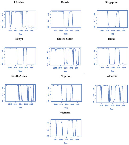
Figure 2.
Filtered probability of Regime 1 (stable market regime) for 10 countries.
In the view of the economic cycles of ten countries, when an economic crisis or a major shock occurs, all countries enter an economic downturn at approximately the same period, but the persistence of the turbulent regime is different. For example, in 2014–2016, there was a 70% drop in oil prices known as the ‘crude shock’ crisis, which was one of the three sharpest drops in oil price after World War II [71,75]. Following the event, almost all countries went from Regime 1 to Regime 2 (See Figure 2). However, the persistence was different. While Regime 2 lasted more than 12 months for Russia, Singapore, Kenya, India, Nigeria, and Vietnam, Regime 2 lasted fewer months for the United States, South Africa, and Colombia. The inflation also fluctuated more during 2014–2016 for the United States, South Africa, and Colombia.
In the third quarter of 2018, all countries changed their status from a stable to a turbulent regime again as they faced the trade conflict between China and the United States that started in January 2018 [76]. The impact of the trade conflict was not limited to China and the United States (European Commission, 2018). The persistence of Regime 2 also differed across countries. The United States, South Africa, Colombia, and Vietnam only faced a short-term contractionary state and experienced an economic upturn before the COVID-19 crisis occurred. On the contrary, Ukraine, Russia, Singapore, Kenya, India, and Nigeria faced a persistent economic downturn from the third quarter of 2018 to the first quarter of 2021.
From the three events, Russia, Singapore, Kenya, India, and Nigeria have exhibited similar characteristics of the transition and persistence of the two regimes, where there were prolonged economic downturns after major economic shocks. In contrast, the United States, South Africa, and Colombia faced shorter periods of shocks and more fluctuations across regimes. Ukraine and Vietnam were found to have different patterns of the business cycle compared with other countries.
In sum, the modified likelihood ratio test and the filtered probabilities plots show strong evidence of the existence of two regimes in the relationship between inflation, stock, Bitcoin, gold, and oil. Thus, we cannot ignore this structural change behavior in testing the hedging potential of Bitcoin and other traditional assets.
5.2. Main Results of the Inflation Hedging Property of BITCOIN and Other Assets
We assume two different states for this work (. Note that the economic interpretations of and can be done by considering the regime-dependent variance and mean parameters in Regimes 1 and 2 (see Table A1, Table A2, Table A3 and Table A4 in Appendix A). We can observe that the variances of Regime 1 are mostly lower than those of Regime 2 (Table A3 and Table A4), while the means of Regime 1 are mostly higher than those of Regime 2 (Table A1 and Table A2). Therefore, the regimes with low volatility and high returns capture the stable market and those with high volatility and low returns regimes coincide with the turbulent market.
We then set off to answer the question: do Bitcoin and traditional assets possess inflation hedging properties differently in stable and turbulent market regimes? This question can be answered by considering the estimated parameters in the MS-VAR model. Note that if the inflation is significantly and positively correlated to the asset return, this asset is considered an inflationary hedge. Specifically, asset can be used to hedge against inflation in state , if the long-run elasticity of asset returns with respect to inflation is significantly positive. There are three levels of ability to hedge depending on the size of the elasticity of asset return coefficient, which is partial hedge (), full hedge (), and superior performance () [77]. The ability for each asset to be used as inflation hedging instruments in stable market and turbulent market regimes are presented in Table 2 and Table 3. To simplify the results, we provide only the estimated coefficients measuring the effect of inflation on each asset’s return for Regimes 1 and 2 in Table 2 and Table 3, respectively.
Table 3.
Estimated parameters and standard errors for Regime 1.
Regarding Regime 1 or the stable market regime, Table 3 shows that stock, Bitcoin, gold, and oil cannot hedge against inflation in most countries. The exception includes Bitcoin, which can hedge against inflation in the United States and Vietnam. The coefficients are significant and greater than one in both cases, indicating that Bitcoin can hedge against inflation. That is, the return of Bitcoin (BTC/USD) increases by 1.2030% and 1.5993% when the inflation increases by 1% in the United States and Vietnam, respectively. This implies that the Bitcoin return increases more than a proportionate increase in the inflation rate. In addition, oil can be used to hedge against inflation in Nigeria. For the case of oil and stock, there is no evidence that these assets are effective inflation hedging instruments in stable market periods.
In the second regime or turbulent regime, Table 4 reveals that stocks, Bitcoin, gold, and oil can hedge against inflation in more countries than in Regime 1. Similar to Regime 1, Bitcoin can hedge against inflation in more countries than other assets. Specifically, Bitcoin can hedge against inflation in four countries, including Nigeria, Ukraine, Kenya, and India, with coefficients greater than one. In terms of stock, there is evidence of Fisher’s effect in Ukraine, India, and Nigeria, as this asset provides a good hedge against inflation. Considering the gold-inflation hedging potential, the result shows that gold provides a good hedge for inflation in the United States and Nigeria, given that the hedging coefficients are significant and positive. Finally, in the case of oil, we find that oil is able to hedge against inflation in Kenya and Ukraine.
Table 4.
Estimated parameters and standard errors for Regime 2.
Based on these two-regime results, we can conclude that there is some evidence of Fisher’s effect on all hedging assets. Specifically, Bitcoin, oil, gold, and stock are either superior performance or partially effective in hedging against inflation in some countries across stable and turbulent regimes. However, the hedging performance of these assets are more effective in the turbulent regime. It is noticeable that positive and negative coefficients of the inflation rate are significantly different in some countries, implying that there is inflation asymmetry in the asset–inflation hedging nexus. This is in agreement with the results of nonlinearity for gold from Beckmann and Czuda [31] and for stock in Hondroyiannis and Papapetrou [65]. The reasons for supporting these results should be that the rigidity adjustment between hedging assets and inflation across the two regimes are different. The cross elasticity between these four assets and inflation is relatively low in a stable regime. Therefore, the adjustment of price presents rigidity. On the other hand, during the turbulent market, the cross-elasticity of assets and inflation is high. As the assets and inflation almost adjust synchronously, the rigidity does not appear in this regime, allowing the investment in these assets to hedge against inflation [7]. We would like to note that this explanation is held in only some countries. Notably, there is no evidence of a positive and significant hedging coefficient in Russia, Singapore, or Columbia. It is noticeable that negative or positive coefficients of the inflation rate are not significantly different. This indicates that there is no inflation asymmetry in the asset–inflation hedging nexus for Russia, Singapore, and Columbia. The possible reason is that the inflation rate of these countries is quite stable [14].
Finally, when we compare the hedging potential of all assets, we find that Bitcoin has worked better against inflation and better than other assets. This is due to the limited supply and decentralization, which bring in the scarcity and resilience power of Bitcoin against inflation [50,51]. However, our results suggest that Bitcoin could offer hedging inflation only in limited circumstances and countries. For example, we find that the ability to inflation hedge Bitcoin according to is not continuous in Regime 2 for the United States and Vietnam. We can observe that the long-run relations between inflation and Bitcoin are 1.2030 and 1.5993 for the United States and Vietnam, respectively, in the first regime but become negative in the second regime. Overall, it seems that the nonlinear structure of the dynamics between inflation and asset prices is confirmed in our analysis. This result also is consistent with those previously obtained findings of Blau et al. [15], who also suggested that the hedging capacity of Bitcoin is primarily associated with some events, such as the COVID-19 pandemic, and does not extend throughout the history of Bitcoin.
5.3. Impulse Response Function (IRF)
In this section, we further investigate the inflation hedging effectiveness of all assets and the effective period of the hedge. By doing this, the regime-dependent impulse response analysis [78] is applied for both stable and turbulent regimes. This analysis allows us to understand how each hedging asset responds to inflation shocks. More precisely, we can examine the size, speed, and duration of the response of Bitcoin, oil, gold, and stock indices to the shock of inflation across both bear and bull regimes.
To detect the hedging potential of assets, we can look at the response of the asset to the shock of the inflation. If an asset responds to an inflation shock in a positive direction, then the asset is not devalued with inflation and can be used to hedge against inflation. In contrast, if an asset responds negatively, the asset is devalued by inflation and cannot hedge against inflation.
Figure 3 and Figure 4 illustrate the impulse response of Bitcoin to the one-standard-deviation shock of inflation for Regimes 1 and 2, respectively. We find that the responses of Bitcoin to shocks in inflation are a bit different across the two regimes. The responses of Bitcoin to inflation shocks are much stronger in the stable regime (Regime 1) than the turbulent regime (Regime 2), as the peak response values of Bitcoin to inflation shocks range from 0.01 (Columbia) to 0.05 (Vietnam) basis points in month two. In contrast, in Regime 1, the response values range from −0.01 (Colombia) to 0.04 (Ukraine) basis points in month two. Overall, in Regime 1, Bitcoin could be useful to hedge against inflation in the short run in all countries except for Columbia; the response of Bitcoin against the inflation shocks of these countries is positive and reaches the highest in month two, and it falls gradually after this month, then tapers off to near zero by months 8–10. Notably, in Columbia, bitcoin can hedge against inflation only in the first two months and lost its ability to hedge in the third month and converged to the original state in eight months.
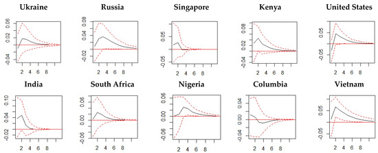
Figure 3.
The impulse response of Bitcoin to the one−standard−deviation shock of inflation in Regime 1. Note: the red dashed line is 95% bootstrap confident interval; the units of the horizontal axes are a month.
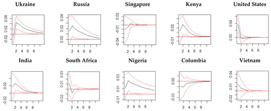
Figure 4.
The impulse response of Bitcoin to the one−standard−deviation shock of inflation in Regime 2. Note: the red dashed line is 95% bootstrap confident interval; the units of the horizontal axes are a month.
For the second regime, Bitcoin can act as a hedge against in Ukraine, Russia, Kenya, India, Nigeria, and Vietnam. Economically, a one-standard-deviation increase in the inflation rate of these countries is associated with an increase in the Bitcoin return. The positive responses of these countries are quite persistent as the responses remain positive for at least 8–10 months. By contrast, the response of Bitcoin to the United States’ inflation is sluggish as it reacts positive in the first month and its response fades out near zero and negative by month two. This indicates that bitcoin can partially hedge against US inflation only in the first month.
Considering other assets—oil, gold, and stock—the impulse response illustrations are provided in Figure 5, Figure 6, Figure 7, Figure 8, Figure 9 and Figure 10. Figure 5 shows the impulse response of stock to the inflation shock in Regime 1. The stock return of each country responds to inflation shock differently. In the case of Russia and South Africa, the stock return can hedge against inflation shocks in the short run for eight months and five months, respectively, before converging to their original states. On the other hand, the stock can only partially hedge against inflation shocks for India and Vietnam. Specifically, the stock can only hedge against inflation for one month and no longer has the hedging potential from the second month. In the United States, the ability to hedge against inflation in the short run is unstable. When there is an inflation shock, it can hedge against inflation in the first two months. Then, during the third month, the stock loses its ability to hedge. However, after the fourth month, the stock index resumes its ability to hedge against inflation shocks and returns to its long-run state in eight months. In Ukraine, Singapore, Kenya, and Columbia, stock indices cannot be used for inflation hedging against inflation shocks.
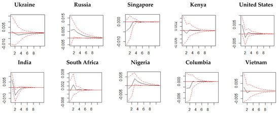
Figure 5.
The impulse response of stock to the one−standard−deviation shock of inflation in Regime 1. Note: red dashed line is 95% bootstrap confident interval; the units of the horizontal axes are a month.
Figure 6 shows the impulse response of gold to the inflation shock in Regime 1. Similar to the stock, the gold price responds differently to inflation shocks in different countries. In particular, gold can hedge against inflation shocks in South Africa and Vietnam. It also can partially hedge in Nigeria, Singapore, Kenya, the United States, Ukraine, Russia, and Columbia, but with different patterns. Specifically, gold can hedge against inflation shocks in Nigeria, except only in a few intermittent periods. For Singapore, Kenya, and the United States, gold can be used as a hedging tool in the initial periods after the inflation shocks occur and then lose its ability to hedge. Conversely, in Ukraine, Russia, and Columbia, gold does not have the hedging property in the initial periods after the shocks but can hedge in later periods before converging to its long-run state. Lastly, gold cannot hedge inflation shocks in the case of India.
Figure 7 shows the impulse response of oil to the inflation shock in Regime 1. In Ukraine, the United States, and South Africa, oil can hedge against inflation shocks for eight months before converging to the origin state. In Kenya, Columbia, and Vietnam, oil can be used to hedge only in the initial periods after the shock and then it loses its ability to hedge. Conversely, in Nigeria, oil cannot hedge against inflation in the initial period but can be used to hedge in the later periods. Lastly, in Russia, Singapore, and India, oil cannot hedge for inflation shocks in the short run.
Figure 8 shows the impulse response of stock to the inflation shock in Regime 2. In Ukraine, India, and Nigeria, stock indices can hedge against inflation shocks. However, the positive impulses last longer than eight months before converging to the original state in the case of Ukraine and Nigeria, while it only lasts shorter than eight months in India. In the case of partial hedging ability, stock indices can hedge against inflation shock in the initial periods but not in the later period before converging into the original state. For Singapore and the United States, the ability to hedge inflation in the short run is unstable. The stock index is not a useful inflation hedge tool in Kenya after inflation shocks.
Figure 9 shows the impulse response of gold to the inflation shock in Regime 2. In Kenya and Columbia, gold could be used for an inflation hedge. In India and South Africa, gold can hedge against inflation shocks in the initial periods but is not qualified as an inflation hedge in the later period. Oppositely, in Ukraine, Russia, Nigeria, and Vietnam, gold cannot hedge against inflation shocks in the initial periods but can hedge in the later periods. In the United States, the ability of gold to hedge inflation in the short run is unstable. Lastly, gold cannot hedge against inflation shocks in Singapore.
Figure 10 shows the impulse response of oil to the inflation shock in Regime 2. Oil can hedge against inflation shocks for longer than six months in Singapore, India, and Nigeria before converging to the origin state. In the United States and Vietnam, oil can be used to hedge against inflation shocks in the initial periods but not the later periods. Conversely, in Columbia, the oil fails to hedge against inflation initially but can be used as an inflation hedging tool in the later periods before converging into the original state. Finally, in Ukraine, Russia, Kenya, and South Africa, oil absolutely could not hedge against inflation shocks.
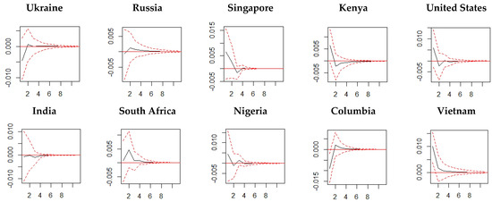
Figure 6.
The impulse response of gold to the one−standard−deviation shock of inflation in Regime 1. Note: red dashed line is 95% bootstrap confident interval; the units of the horizontal axes are a month.
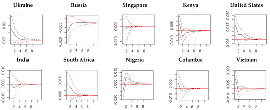
Figure 7.
The impulse response of oil to the one−standard−deviation shock of inflation in Regime 1. Note: red dashed line is 95% bootstrap confident interval; the units of the horizontal axes are a month.
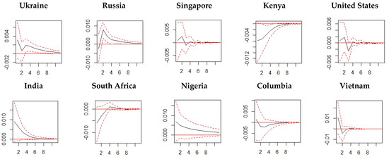
Figure 8.
The impulse response of stock to the one−standard−deviation shock of inflation in Regime 2. Note: red dashed line is 95% bootstrap confident interval; the units of the horizontal axes are a month.
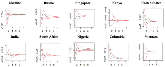
Figure 9.
The impulse response of gold to the one−standard−deviation shock of inflation in Regime 2. Note: red dashed line is 95% bootstrap confident interval; the units of the horizontal axes are a month.
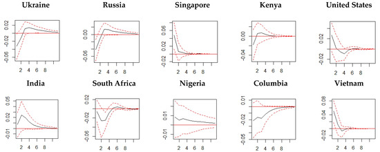
Figure 10.
The impulse response of oil to the one−standard−deviation shock of inflation in Regime 2. Note: red dashed line is 95% bootstrap confident interval; the units of the horizontal axes are a month.
To clearly understand the impulse response analysis results, we summarize the result in Table 5. The left panel of this table shows the long-run hedging ability of each asset against inflation following the hedging coefficient of the MS-VAR , while the right panel shows the result of the short-run hedging ability of each asset against inflation following the MS-VAR’s impulse response. We would like to note that the short-run IRF reveals how rapid asset prices change according to the sudden change in inflation, while the long-run relationship means an equilibrium relationship between each asset and inflation in the long term.
Table 5.
Long-run and short-run hedging ability of different assets in two regimes.
As the interpretation of the long-run coefficient of the MS-VAR model has already been explained in the previous section, we focus on the summarized results in the right panel. The response path of each asset against inflation is reported as the positive (+) and negative (−) signs. “+“ means that the asset can be used to hedge against inflation for at least 10 months, “−“ means that the asset cannot be used to hedge against inflation for at least 10 months, “+ −“ and “− +“ mean that the asset can be used to hedge against inflation at the beginning phase and turning to perverse hedge against inflation in the latter phase, and vice versa.
Several observations can be made and summarized as follows: (1) Consistent with results from previous studies, all assets can hedge against inflation more effectively in the short run than in the long run [4,58]. We also find that all assets hedge against inflation similarly in both regimes [3,31]. This indicates the existence of temporary hedging ability of the assets in both stable and turbulent regimes. (2) Among the four assets, we observe that Bitcoin plays an important role as a hedging asset against inflation in both regimes as the response of Bitcoin is positive and persistent in 7 and 5 countries out of 10 countries in stable and turbulent regimes, respectively. The finding that bitcoin can hedge against inflation is consistent with Choi and Shin [8], who also report Bitcoin appreciates against inflation (or inflation expectation) shocks in the United States. (3) In contrast, the hedging performance of gold, oil, and stock is quite similar and low as their responses are not persistently positive 10 months after the inflation shock. This stance is similar to the findings of Salisu at el. [14] for gold, Ivanov [79] for stock, and Zaremba et al. [40] for oil. (4) All assets can be used to hedge against inflation in the United States for some periods of time as the responses of the assets against inflation swing between negative and positive before reaching the long-run equilibrium. This is also confirmed by the fact that there is no long-run hedging ability of three out of four assets in the United States, as shown in the left panel. The same situation is found in South Africa in the second regime.
In sum, an overview of results in Table 5 shows that inflation hedging tendencies are heterogeneous to various classifications of assets. While the short run validates Fisher’s hypothesis, the same cannot be concluded for the long run. It is also interesting to remark that these results hold after accounting for features such as structural breaks and nonlinearity.
6. Conclusions, Policy Implication and Limitation, and Future Research
Although, there is a widespread belief that gold, stock, and oil may act as an inflation hedge, the empirical evidence is mixed. Bitcoin is another asset that has become a significant interest among the academia and policymakers; however, existing theoretical and empirical studies have not reached a consensus about its hedging ability [8]. This may be due to the differences in methodology, the time horizon, and the characteristics of the economy under consideration in the analysis, given the conflicting opinions regarding Bitcoin, gold, stock, and oil as a potential inflation hedge. Therefore, this study re-examines whether these assets can hedge against inflation in ten countries with the highest rate of cryptocurrency adoption in the stable and turbulent regimes using the Markov Switching Vector Autoregressive Regression (MS-VAR).
Our results first reveal that the structural change and nonlinear relationship between hedging assets and inflation should be taken into account when examining the hedging potential of Bitcoin, gold, stock, and oil. We notice that the structural change is detected by the Markov process and modified likelihood ratio test.
An overview of the results of the long-run coefficients and regime-dependent impulse response (short-run) shows that inflation hedging tendencies are heterogeneous to various classifications of assets, and it is hard to find an asset that can effectively hedge against inflation in the long run, especially when the economy faces a stable market regime. However, holding Bitcoin, gold, stocks, or oil can hedge against inflation shocks in the short run. When comparing Bitcoin with other traditional inflation hedging assets, Bitcoin tends to be able to hedge against inflation shocks more effectively than other assets for countries with high cryptocurrency adoption.
Based on the empirical results, there are two main recommendations. Firstly, this study finds that all assets can hedge against inflation more effectively in the short run than in the long run. Therefore, investors should adjust their portfolios to incorporate assets with inflation hedging properties after inflation shocks. However, the choice of assets and the length of asset holding periods differ significantly across countries. In the long run, the ability of investors to hedge against inflation is limited in most countries. From a policymaker’s point of view, the essential keys of inflation hedge are time selection and asset selection. Policymakers should consider making a hedge against inflation in the time of market downturn or time when asset prices respond to inflation faster to avoid inflation. Secondly, the results show that bitcoin is an effective inflation hedging instrument in more countries than other assets in stable and turbulent regimes. This evidence of Bitcoin’s ability to hedge for inflation is a benefit that each government should consider when developing cryptocurrency regulations.
The main limitation of this study is the frequency of inflation data. While data for all asset prices are high frequency, the data for inflation are monthly. Future studies can examine the possibility of using a frequency mismatch estimation model to capture the higher-frequency variation of asset prices. Alternatively, it can also be useful to transform the inflation data into a higher-frequency variable using proxies or forecasting methods. This will allow us to examine shorter-term inflation-hedging strategies. In addition, changing the order of variables in the MS-VAR system may change the results to be obtained [80]. It may be difficult to discuss the robustness of the results when the order is changed. To obtain a reliable result for the MS-VAR model, more attention is needed for the order of the variables in the MS-VAR system. For further studies, the Markov Switching Structural VAR model is suggested to investigate the variable ordering issue.
Author Contributions
P.P., S.L. and N.P carried out the literature review, statistical analysis, and drafted the manuscript. S.L. and N.P. helped with the data collections, data analysis, and discussion. P.P. and S.L. made major contributions to writing the manuscript and W.Y. prepared the computer code and estimation. All authors have read and agreed to the published version of the manuscript.
Funding
This research received no external funding.
Data Availability Statement
The inflation data are obtained from International Financial Statistics (IFS) and the data for Bitcoin (BTC/USD), gold (XAU/USD), oil (Brent/USD), and stock prices are obtained from investing.com (accessed on 25 November 2021).
Acknowledgments
This paper is supported by the Center of Excellence in Econometrics, Faculty of Economics, Chiang Mai University and the School of Business and Communication Arts, University of Phayao.
Conflicts of Interest
The authors declare no conflict of interest.
Appendix A
Table A1.
Estimated intercept term for Regime 1.
Table A1.
Estimated intercept term for Regime 1.
| Inflation | Stock | Bitcoin | Gold | Oil | |
|---|---|---|---|---|---|
| Ukraine | 0.0049 *** | −0.0017 | 0.0857 ** | 0.0047 | −0.0031 |
| (0.0017) | (0.0095) | (0.0391) | (0.0050) | (0.0085) | |
| Russia | 0.0024 *** | 0.0185 * | 0.0569 | 0.0030 | −0.0036 |
| (0.0006) | (0.0063) | (0.0491) | (0.0062) | (0.0090) | |
| Singapore | 0.0025 *** | 0.0004 | 0.1145 *** | 0.0009 | 0.0124 ** |
| (0.0004) | (0.0046) | (0.0392) | (0.0046) | (0.0060) | |
| Kenya | 0.0034 *** | 0.0120 *** | 0.0834 ** | 0.0047 | 0.0206 *** |
| (0.0007) | (0.0048) | (0.0469) | (0.0056) | (0.0069) | |
| United States | 0.0012 *** | 0.0163 *** | 0.0505 * | 0.0062 | 0.0100 |
| (0.0002) | (0.0031) | (0.0355) | (0.0049) | (0.0080) | |
| India | 0.0047 *** | 0.0247 *** | 0.0822 ** | 0.0007 | 0.0164 *** |
| (0.0007) | (0.0044) | (0.0424) | (0.0053) | (0.0066) | |
| South Africa | 0.0033 *** | 0.0162 *** | 0.0568 | 0.0008 | 0.0043 |
| (0.0004) | (0.0046) | (0.0469) | (0.0062) | (0.0107) | |
| Nigeria | 0.0094 *** | 0.0039 | 0.1212 * | 0.0063 | 0.0142 |
| (0.0010) | (0.0092) | (0.0817) | (0.0100) | (0.0115) | |
| Columbia | 0.0013 *** | 0.0046 | 0.1458 *** | 0.0020 *** | 0.0157 ** |
| (0.0002) | (0.0048) | (0.0463) | (0.0059) | (0.0085) | |
| Vietnam | 0.0020 *** | 0.0118 ** | 0.0654 *** | 0.0076 | 0.0166 *** |
| (0.0005) | (0.0058) | (0.0298) | (0.0051) | (0.0064) |
Note: (1) Standard errors in parentheses. (2) ***, **, * represent significance levels at 0.01, 0.05, and 0.1, respectively.
Table A2.
Estimated intercept term for Regime 2.
Table A2.
Estimated intercept term for Regime 2.
| Inflation | Stock | Bitcoin | Gold | Oil | |
|---|---|---|---|---|---|
| Ukraine | 0.0019 *** | −0.0119 *** | 0.0364 ** | −0.0228 *** | −0.0795 *** |
| (0.0005) | (0.0019) | (0.0188) | (0.0038) | (0.0192) | |
| Russia | 0.0022 *** | −0.0154 *** | 0.0482 ** | −0.0052 | −0.0419 ** |
| (0.0006) | (0.0063) | (0.0491) | (0.0062) | (0.0090) | |
| Singapore | 0.0002 | −0.0055 * | 0.0427 *** | −0.0031 | −0.0181 |
| (0.0003) | (0.0041) | (0.0168) | (0.0040) | (0.0167) | |
| Kenya | 0.0035 *** | −0.0129 *** | 0.0176 | −0.0032 | −0.0144 |
| (0.0005) | (0.0054) | (0.0207) | (0.0050) | (0.0210) | |
| United States | 0.0004 *** | 0.0065 | 0.0122 | 0.0011 | −0.0033 |
| (0.0481) | (1.7070) | (0.7123) | (1.2834) | (4.3423) | |
| India | 0.0023 *** | 0.0006 | 0.0224 | −0.0064 * | −0.0403 *** |
| (0.0007) | (0.0044) | (0.0424) | (0.0053) | (0.0066) | |
| South Africa | 0.0030 *** | 0.0023 | 0.0412 *** | −0.0086 ** | 0.0508 *** |
| (0.0004) | (0.0066) | (0.0234) | (0.0051) | (0.0224) | |
| Nigeria | 0.0024 *** | −0.0577 *** | −0.0770 ** | −0.0180 *** | −0.0262 |
| (0.0004) | (0.0132) | (0.0347) | (0.0073) | (0.0307) | |
| Columbia | 0.0011 *** | −0.0122 ** | 0.0153 | 0.0063 | 0.0281 |
| (0.0003) | (0.0085) | (0.0219) | (0.0058) | (0.0230) | |
| Vietnam | 0.0014 *** | 0.0078 | 0.0528 *** | 0.0047 | −0.0206 |
| (0.0003) | (0.0072) | (0.0189) | (0.0044) | (0.0185) |
Note: (1) Standard errors in parentheses. (2) ***, **, * represent significance levels at 0.01, 0.05, and 0.1, respectively.
Table A3.
Estimated variance for Regime 1.
Table A3.
Estimated variance for Regime 1.
| Inflation | Stock | Bitcoin | Gold | Oil | |
|---|---|---|---|---|---|
| Ukraine | 0.0006 *** | 0.0003 *** | 0.2324 * | 0.0024 | 0.0338 *** |
| (0.0002) | (0.0001) | (0.1222) | (0.0023) | (0.0012) | |
| Russia | 0.00021 ** | 0.0016 | 0.2283 ** | 0.0027 ** | 0.0339 *** |
| (0.00007) | (0.0010) | (0.1022) | (0.0011) | (0.0021) | |
| Singapore | 0.00032 * | 0.0019 | 0.2313 ** | 0.0027 ** | 0.0308 |
| (0.00019) | (0.0050) | (0.1120) | (0.0010) | (0.0230) | |
| Kenya | 0.00024 *** | 0.0021 ** | 0.1305 | 0.0028 | 0.0316 |
| (0.00010) | (0.0011) | (0.2990) | (0.0222) | (0.0231) | |
| United States | 0.00019 *** | 0.0038 *** | 0.2314 * | 0.0026 ** | 0.0181 |
| (0.00006) | (0.0012) | (0.1230) | (0.0012) | (0.0234) | |
| India | 0.00012 *** | 0.0031 | 0.3309 *** | 0.0028 | 0.0258 |
| (0.00004) | (0.0021) | (0.1129) | (0.0021) | (0.0192) | |
| South Africa | 0.00017 | 0.0023 ** | 0.2289 ** | 0.0024 | 0.0264 |
| (0.00012) | (0.0010) | (0.1122) | (0.0022) | (0.0222) | |
| Nigeria | 0.00021 *** | 0.0047 * | 0.2330 ** | 0.0035 * | 0.0257 ** |
| (0.0005) | (0.0023) | (0.1193) | (0.0019) | (0.0109) | |
| Columbia | 0.00010 | 0.0044 ** | 0.2292 *** | 0.0024 | 0.0323 |
| (0.0013) | (0.0019) | (0.0604) | (0.0020) | (0.0213) | |
| Vietnam | 0.00022 *** | 0.0044 *** | 0.1302 | 0.0027 | 0.0290 |
| (0.00014) | (0.0015) | (0.0909) | (0.0039) | (0.0211) |
Note: (1) Standard errors in parentheses. (2) ***, **, * represent significance levels at 0.01, 0.05, and 0.1, respectively.
Table A4.
Estimated variance for Regime 2.
Table A4.
Estimated variance for Regime 2.
| Inflation | Stock | Bitcoin | Gold | Oil | |
|---|---|---|---|---|---|
| Ukraine | 0.0004 *** | 0.0083 *** | 0.1401 *** | 0.0023 ** | 0.0067 *** |
| (0.0001) | (0.0021) | (0.0340) | (0.0010) | (0.0022) | |
| Russia | 0.00013 *** | 0.0024 | 0.1444 | 0.0023 | 0.0048 * |
| (0.00007) | (0.0020) | (0.1001) | (0.0022) | (0.0021) | |
| Singapore | 0.00021 *** | 0.0024 | 0.1702 *** | 0.0024 ** | 0.0040 |
| (0.00009) | (0.0023) | (0.0245) | (0.0011) | (0.0044) | |
| Kenya | 0.00023 | 0.0016 | 0.1572 ** | 0.0023 | 0.0034 *** |
| (0.00021) | (0.0011) | (0.0824) | (0.0034) | (0.0016) | |
| United States | 0.00016 *** | 0.0009 *** | 0.1128 *** | 0.0021 | 0.0057 |
| (0.00003) | (0.0003) | (0.0535) | (0.0020) | (0.0031) | |
| India | 0.00011 *** | 0.0016 | 0.1491 | 0.0023 ** | 0.0036 |
| (0.00005) | (0.0022) | (0.1002) | (0.0011) | (0.0030) | |
| South Africa | 0.00007 | 0.0011 *** | 0.1160 *** | 0.0021 | 0.0061 *** |
| (0.0002) | (0.0005) | (0.0245) | (0.0016) | (0.0022) | |
| Nigeria | 0.00015 *** | 0.0023 * | 0.1825 | 0.0028 *** | 0.0036 ** |
| (0.00006) | (0.0011) | (0.9234) | (0.0010) | (0.0017) | |
| Columbia | 0.00006 *** | 0.0014 *** | 0.1309 | 0.0021 ** | 0.0044 |
| (0.00002) | (0.0004) | (0.1092) | (0.0011) | (0.0053) | |
| Vietnam | 0.00017 | 0.0028 | 0.1338 *** | 0.0022 ** | 0.0035 |
| 0.00023 | (0.0022) | (0.0564) | (0.0012) | (0.0031) |
Note: (1) Standard errors in parentheses. (2) ***, **, * represent significance levels at 0.01, 0.05, and 0.1, respectively.
References
- Altissimo, F.; Benigno, P.; Palenzuela, D.R. Inflation differentials in a currency area: Facts, explanations and policy. Open Econ. Rev. 2011, 22, 189–233. [Google Scholar] [CrossRef]
- Tarbert, H. Is commercial property a hedge against inflation? A cointegration approach. J. Prop. Financ. 1996, 7, 77–98. [Google Scholar] [CrossRef]
- Aye, G.C.; Chang, T.; Gupta, R. Is gold an inflation-hedge? Evidence from an interrupted Markov-switching cointegration model. Resour. Policy 2016, 48, 77–84. [Google Scholar] [CrossRef] [Green Version]
- Van Hoang, T.H.; Lahiani, A.; Heller, D. Is gold a hedge against inflation? New evidence from a nonlinear ARDL approach. Econ. Model. 2016, 54, 54–66. [Google Scholar] [CrossRef] [PubMed]
- Kaponda, K. Bitcoin the’Digital Gold’and Its Regulatory Challenges. Available online: https://papers.ssrn.com/sol3/papers.cfm?abstract_id=3123531 (accessed on 1 February 2022). [CrossRef]
- Salisu, A.A.; Ndako, U.B.; Oloko, T.F. Assessing the inflation hedging of gold and palladium in OECD countries. Resour. Policy 2019, 62, 357–377. [Google Scholar] [CrossRef]
- Wang, K.M.; Lee, Y.M.; Thi, T.B.N. Time and place where gold acts as an inflation hedge: An application of long-run and short-run threshold model. Econ. Model. 2011, 28, 806–819. [Google Scholar] [CrossRef]
- Choi, S.; Shin, J. Bitcoin: An inflation hedge but not a safe haven. Financ. Res. Lett. 2021, 46, 102379. [Google Scholar] [CrossRef]
- Ciaian, P.; Rajcaniova, M.; Kancs, D.A. The economics of BitCoin price formation. Appl. Econ. 2016, 48, 1799–1815. [Google Scholar] [CrossRef] [Green Version]
- Fisher, I. Theory of Interest: As Determined by Impatience to Spend Income and Opportunity to Invest it; Augustusm Kelly Publishers: Wollongong, Australia, 1930. [Google Scholar]
- Bodie, Z. Common stocks as a hedge against inflation. J. Financ. 1976, 31, 459–470. [Google Scholar] [CrossRef]
- Fama, E.F.; Schwert, G.W. Asset returns and inflation. J. Financ. Econ. 1977, 5, 115–146. [Google Scholar] [CrossRef]
- Bekaert, G.; Wang, X. Inflation risk and the inflation risk premium. Econ. Policy 2010, 25, 755–806. [Google Scholar] [CrossRef]
- Salisu, A.A.; Raheem, I.D.; Ndako, U.B. The inflation hedging properties of gold, stocks and real estate: A comparative analysis. Resour. Policy 2020, 66, 101605. [Google Scholar] [CrossRef]
- Blau, B.M.; Griffith, T.G.; Whitby, R.J. Inflation and Bitcoin: A descriptive time-series analysis. Econ. Lett. 2021, 203, 109848. [Google Scholar] [CrossRef]
- Arnold, S.; Auer, B.R. What do scientists know about inflation hedging? N. Am. J. Econ. Financ. 2015, 34, 187–214. [Google Scholar] [CrossRef]
- Capie, F.; Mills, T.C.; Wood, G. Gold as a hedge against the dollar. J. Int. Financ. Mark. Inst. Money 2005, 15, 343–352. [Google Scholar] [CrossRef]
- Erb, C.B.; Harvey, C.R. The golden dilemma. Financ. Anal. J. 2013, 69, 10–42. [Google Scholar] [CrossRef]
- Ghosh, D.; Levin, E.J.; MacMillan, P.; Wright, R.E. Gold as an inflation hedge? Stud. Econ. Financ. 2004, 22, 1–25. [Google Scholar] [CrossRef] [Green Version]
- Levin, E.J.; Montagnoli, A.; Wright, R.E. Short-run and long-run determinants of the price of gold. World Gold Counc. Res. Study 2006, 32, 1–68. [Google Scholar]
- McCown, J.R.; Zimmerman, J.R. Is gold a zero-beta asset? Analysis of the investment potential of precious metals. Oklahoma City University Working Paper. SSRN Electron. J. 2006. [Google Scholar] [CrossRef]
- McCown, J.R.; Zimmerman, J.R. Analysis of the investment potential and inflation-hedging ability of precious metals. Oklahoma City University Working Paper. SSRN Electron. J. 2007. [Google Scholar] [CrossRef]
- Rubbaniy, G.; Lee, K.T.; Verschoor, W.F. Metal investments: Distrust killer or inflation hedging? In Proceedings of the 24th Australasian Finance and Banking Conference, Sydney, Australia, 14–16 December 2011. [Google Scholar]
- Worthington, A.C.; Pahlavani, M. Gold investment as an inflationary hedge: Cointegration evidence with allowance for endogenous structural breaks. Appl. Financ. Econ. Lett. 2007, 3, 259–262. [Google Scholar] [CrossRef] [Green Version]
- Baur, D.G. Explanatory mining for gold: Contrasting evidence from simple and multiple regressions. Resour. Policy 2011, 36, 265–275. [Google Scholar] [CrossRef]
- Blose, L.E. Gold prices, cost of carry, and expected inflation. J. Econ. Bus. 2010, 62, 35–47. [Google Scholar] [CrossRef]
- Brown, K.C.; Howe, J.S. On the use of gold as a fixed income security. Financ. Anal. J. 1987, 43, 73–76. [Google Scholar] [CrossRef]
- Mahdavi, S.; Zhou, S. Gold and commodity prices as leading indicators of inflation: Tests of long-run relationship and predictive performance. J. Econ. Bus. 1997, 49, 475–489. [Google Scholar] [CrossRef]
- Aye, G.C.; Carcel, H.; Gil-Alana, L.A.; Gupta, R. Does gold act as a hedge against inflation in the UK? Evidence from a fractional cointegration approach over 1257 to 2016. Resour. Policy 2017, 54, 53–57. [Google Scholar] [CrossRef]
- Batten, J.A.; Ciner, C.; Lucey, B.M. On the economic determinants of the gold–inflation relation. Resour. Policy 2014, 41, 101–108. [Google Scholar] [CrossRef]
- Beckmann, J.; Czudaj, R. Gold as an inflation hedge in a time-varying coefficient framework. N. Am. J. Econ. Financ. 2013, 24, 208–222. [Google Scholar] [CrossRef] [Green Version]
- Chua, J.; Woodward, R.S. Gold as an inflation hedge: A comparative study of six major industrial countries. J. Bus. Financ. Account. 1982, 9, 191–197. [Google Scholar] [CrossRef]
- Jaffe, J.F. Gold and gold stocks as investments for institutional portfolios. Financ. Anal. J. 1989, 45, 53–59. [Google Scholar] [CrossRef]
- Lucey, B.M.; Sharma, S.S.; Vigne, S.A. Gold and inflation (s)–A time-varying relationship. Econ. Model. 2017, 67, 88–101. [Google Scholar] [CrossRef] [Green Version]
- Shahzad, S.J.H.; Bouri, E.; Roubaud, D.; Kristoufek, L.; Lucey, B. Is Bitcoin a better safe-haven investment than gold and commodities? Int. Rev. Financ. Anal. 2019, 63, 322–330. [Google Scholar] [CrossRef]
- Taylor, N.J. Precious metals and inflation. Appl. Financ. Econ. 1998, 8, 201–210. [Google Scholar] [CrossRef]
- Adrangi, B.; Chatrath, A.; Raffiee, K. Economic activity, inflation, and hedging: The case of gold and silver investments. J. Wealth Manag. 2003, 6, 60–77. [Google Scholar] [CrossRef]
- Gupta, P.; Goyal, A. Impact of oil price fluctuations on Indian economy. OPEC Energy Rev. 2015, 39, 141–161. [Google Scholar] [CrossRef]
- Hijazine, R.; Al-Assaf, G. The effect of oil prices on headline and core inflation in Jordan. OPEC Energy Rev. 2022. [Google Scholar] [CrossRef]
- Zaremba, A.; Umar, Z.; Mikutowski, M. Inflation hedging with commodities: A wavelet analysis of seven centuries worth of data. Econ. Lett. 2019, 181, 90–94. [Google Scholar] [CrossRef]
- Gultekin, N.B. Stock market returns and inflation: Evidence from other countries. J. Financ. 1983, 38, 49–65. [Google Scholar] [CrossRef]
- Jaffe, J.F.; Mandelker, G. The” Fisher effect” for risky assets: An empirical investigation. J. Financ. 1976, 31, 447–458. [Google Scholar] [CrossRef]
- Luintel, K.B.; Paudyal, K. Are common stocks a hedge against inflation? J. Financ. Res. 2006, 29, 1–19. [Google Scholar] [CrossRef]
- Nelson, C.R.; Schwert, G.W. Short-term interest rates as predictors of inflation: On testing the hypothesis that the real rate of interest is constant. Am. Econ. Rev. 1977, 67, 478–486. [Google Scholar]
- Rödel, M.G. Inflation Hedging. An Empirical Analysis on Inflation Nonlinearities, Infrastructure, and International Equities. Ph.D. Thesis, Technical University of Munich, Munich, Germany, 2012. [Google Scholar]
- Rödel, M.G. Inflation hedging with international equities. J. Portf. Manag. 2014, 40, 41–53. [Google Scholar] [CrossRef]
- Schotman, P.C.; Schweitzer, M. Horizon sensitivity of the inflation hedge of stocks. J. Empir. Financ. 2000, 7, 301–315. [Google Scholar] [CrossRef]
- Hoesli, M.; Lizieri, C.; MacGregor, B. The inflation hedging characteristics of US and UK investments: A multi-factor error correction approach. J. Real Estate Financ. Econ. 2008, 36, 183–206. [Google Scholar] [CrossRef] [Green Version]
- Simpson, M.W.; Ramchander, S.; Webb, J.R. The asymmetric response of equity REIT returns to inflation. J. Real Estate Financ. Econ. 2007, 34, 513–529. [Google Scholar] [CrossRef]
- Bouri, E.; Molnár, P.; Azzi, G.; Roubaud, D.; Hagfors, L.I. On the hedge and safe haven properties of Bitcoin: Is it really more than a diversifier? Financ. Res. Lett. 2017, 20, 192–198. [Google Scholar] [CrossRef]
- Bouri, E.; Gupta, R.; Tiwari, A.K.; Roubaud, D. Does Bitcoin hedge global uncertainty? Evidence from wavelet-based quantile-in-quantile regressions. Financ. Res. Lett. 2017, 23, 87–95. [Google Scholar] [CrossRef] [Green Version]
- Corbet, S.; Meegan, A.; Larkin, C.; Lucey, B.; Yarovaya, L. Exploring the dynamic relationships between cryptocurrencies and other financial assets. Econ. Lett. 2018, 165, 28–34. [Google Scholar] [CrossRef] [Green Version]
- Dyhrberg, A.H. Hedging capabilities of bitcoin. Is it the virtual gold? Financ. Res. Lett. 2016, 16, 139–144. [Google Scholar] [CrossRef] [Green Version]
- Huynh, T.L.D.; Ahmed, R.; Nasir, M.A.; Shahbaz, M.; Huynh, N.Q.A. The nexus between black and digital gold: Evidence from US markets. Ann. Oper. Res. 2021, 1–26. [Google Scholar] [CrossRef]
- Selmi, R.; Mensi, W.; Hammoudeh, S.; Bouoiyour, J. Is Bitcoin a hedge, a safe haven or a diversifier for oil price movements? A comparison with gold. Energy Econ. 2018, 74, 787–801. [Google Scholar] [CrossRef]
- Taskinsoy, J. Bitcoin Nation: The World’s New 17th Largest Economy. Available online: https://www.researchgate.net/publication/349669164_Bitcoin_Nation_The_World%27s_New_17th_Largest_Economy (accessed on 1 February 2022). [CrossRef]
- Matkovskyy, R.; Jalan, A. Bitcoin vs Inflation: Can Bitcoin Be a Macro Hedge? Evidence From a Quantile-on-Quantile Model. SSRN Electron. J. 2020, 7, 1021–1039. [Google Scholar] [CrossRef]
- Smales, L.A. Cryptocurrency as an Alternative Inflation Hedge? 2021. Available online: https://papers.ssrn.com/sol3/papers.cfm?abstract_id=3883123 (accessed on 20 November 2021).
- Conlon, T.; Corbet, S.; McGee, R.J. Inflation and cryptocurrencies revisited: A time-scale analysis. Econ. Lett. 2021, 206, 109996. [Google Scholar] [CrossRef]
- Ghazali, M.F.; Lean, H.H.; Bahari, Z. Is gold a good hedge against inflation? Empirical evidence in Malaysia. J. Malays. Stud. 2015, 33, 69–84. [Google Scholar]
- Le Long, H.; De Ceuster, M.J.; Annaert, J.; Amonhaemanon, D. Gold as a hedge against inflation: The Vietnamese case. Procedia Econ. Financ. 2013, 5, 502–511. [Google Scholar] [CrossRef] [Green Version]
- Maneejuk, P.; Pirabun, N.; Singjai, S.; Yamaka, W. Currency Hedging Strategies Using Histogram-Valued Data: Bivariate Markov Switching GARCH Models. Mathematics 2021, 9, 2773. [Google Scholar] [CrossRef]
- Kim, J.H.; Ryoo, H.H. Common stocks as a hedge against inflation: Evidence from century-long US data. Econ. Lett. 2011, 113, 168–171. [Google Scholar] [CrossRef]
- Ihle, R.; von Cramon-Taubadel, S. A comparison of threshold cointegration and Markov-switching vector error correction models in price transmission analysis (No. 1314-2016-102645). In Proceedings of the 2008 NCCC-134 Conference on Applied Commodity Price Analysis, Forecasting, and Market Risk Management, St. Louis, MI, USA, 21–22 April 2008. [Google Scholar]
- Hondroyiannis, G.; Papapetrou, E. Stock returns and inflation in Greece: A Markov switching approach. Rev. Financ. Econ. 2006, 15, 76–94. [Google Scholar] [CrossRef]
- Krolzig, H.M. The markov-switching vector autoregressive model. In Markov-Switching Vector Autoregressions; Springer: Berlin/Heidelberg, Germany, 1997; pp. 6–28. [Google Scholar]
- Hamilton, J.D. A new approach to the economic analysis of nonstationary time series and the business cycle. Econom. J. Econom. Soc. 1989, 57, 357–384. [Google Scholar] [CrossRef]
- Shi, S.P. Specification sensitivities in the Markov-switching unit root test for bubbles. Empir. Econ. 2013, 45, 697–713. [Google Scholar] [CrossRef]
- Hall, S.G.; Psaradakis, Z.; Sola, M. Detecting periodically collapsing bubbles: A Markov-switching unit root test. J. Appl. Econom. 1999, 14, 143–154. [Google Scholar] [CrossRef]
- Alamgir, F.; Amin, S.B. The nexus between oil price and stock market: Evidence from South Asia. Energy Rep. 2021, 7, 693–703. [Google Scholar] [CrossRef]
- Grigoli, F.; Herman, A.; Swiston, M.A.J. A Crude Shock: Explaining the Impact of the 2014–2016 Oil Price Decline Across Exporters. Int. Monet. Fund 2017, 2017, 3–25. [Google Scholar] [CrossRef]
- Hansen, B.E. Erratum: The likelihood ratio test under nonstandard conditions: Testing the Markov switching model of GNP. J. Appl. Econom. 1996, 11, 195–198. [Google Scholar] [CrossRef] [Green Version]
- Anas, J.; Ferrara, L. Detecting cyclical turning points: The ABCD approach and two probabilistic indicators. J. Bus. Cycle Meas. Anal. 2004, 2004, 193–225. [Google Scholar] [CrossRef]
- Artis, M.; Krolzig, H.M.; Toro, J. The European business cycle. Oxf. Econ. Pap. 2004, 56, 1–44. [Google Scholar] [CrossRef] [Green Version]
- Stocker, M.; Baffes, J.; Some, Y.M.; Vorisek, D.; Wheeler, C.M. The 2014-16 oil price collapse in retrospect: Sources and implications. World Bank Policy Res. Work. Pap. 2018, 1, 8419. [Google Scholar]
- Chong, T.T.L.; Li, X. Understanding the China–US trade war: Causes, economic impact, and the worst-case scenario. Econ. Political Stud. 2019, 7, 185–202. [Google Scholar] [CrossRef]
- Bampinas, G.; Panagiotidis, T. Are gold and silver a hedge against inflation? A two century perspective. Int. Rev. Financ. Anal. 2015, 41, 267–276. [Google Scholar] [CrossRef] [Green Version]
- Ehrmann, M.; Ellison, M.; Valla, N. Regime-dependent impulse response functions in a Markov-switching vector autoregression model. Econ. Lett. 2003, 78, 295–299. [Google Scholar] [CrossRef] [Green Version]
- Ivanov, S.I. A study of perfect hedges. Int. J. Financ. Stud. 2017, 5, 28. [Google Scholar] [CrossRef] [Green Version]
- Pastpipatkul, P.; Yamaka, W.; Sriboonchitta, S. Effect of quantitative easing on ASEAN-5 financial markets. In Causal Inference in Econometrics; Springer: Cham, Switzerland, 2016; pp. 525–543. [Google Scholar]
Publisher’s Note: MDPI stays neutral with regard to jurisdictional claims in published maps and institutional affiliations. |
© 2022 by the authors. Licensee MDPI, Basel, Switzerland. This article is an open access article distributed under the terms and conditions of the Creative Commons Attribution (CC BY) license (https://creativecommons.org/licenses/by/4.0/).