Article

Projective Integration for Hyperbolic Shallow Water Moment Equations

by
Amrita Amrita
1 and
Julian Koellermeier
2,3,4,*
1
Department of Mathematics, KU Leuven, 3001 Leuven, Belgium
2
Department of Computer Science, KU Leuven, 3001 Leuven, Belgium
3
Bernoulli Institute for Mathematics, Computer Science and Artificial Intelligence, University of Groningen, Nijenborgh 4, 9747 AG Groningen, The Netherlands
4
Groningen Cognitive Systems and Materials Center, University of Groningen, Nijenborgh 4, 9747 AG Groningen, The Netherlands
*
Author to whom correspondence should be addressed.
Axioms 2022, 11(5), 235; https://doi.org/10.3390/axioms11050235
Submission received: 8 March 2022 / Revised: 28 April 2022 / Accepted: 4 May 2022 / Published: 18 May 2022

Abstract

:
In free surface flows, shallow water models simplify the flow conditions by assuming a constant velocity profile over the water depth. Recently developed Shallow Water Moment Equations allow for variations of the velocity profile at the expense of a more complex PDE system. The resulting equations can become stiff depending on the friction parameters, which leads to severe time step constraints of standard numerical schemes. In this paper, we apply Projective Integration schemes to stiff Shallow Water Moment Equations to overcome the time step constraints in the stiff regime and accelerate the numerical computations while still achieving high accuracy. In different dam break and smooth wave test cases, we obtain a speedup of up to 55 with respect to standard schemes.

1. Introduction

In shallow water models for geophysical free surface flows [1,2], shallowness refers to flows in which the water height is significantly smaller than a typical wavelength. Choosing a vertical average velocity leads to a depth-averaged model [3,4]. In its one-dimensional form, this most famous depth-averaged flow model is referred to as the Saint-Venant equations or Shallow Water Equations (SWE) [4].
However, depth-averaging comes at the price of losing vertical information. Assuming a constant velocity throughout the flow depth, vertical variations in the velocity cannot be represented [3,4]. This results in a model error [5]. To overcome this problem, vertical information can be included via the moment method [4], which assumes a polynomial expansion of the vertical velocity. The resulting shallow water moment equations preserve information on the structure of the vertical flow while still using the depth-averaging framework. The original model from [4] lacks hyperbolicity and several regularized models have been derived in [3]. The development is supported by analytical and numerical stability investigation in [6].
While the transport term and its hyperbolicity have been studied in detail [3], up to this point there is no dedicated investigation on different friction models, besides a brief comparison in [4] and one application to sediment transport [7]. Note that the friction term also plays an important role in the linear stability analysis of the model [6]. Different friction terms introduce numerical problems for standard solution schemes, as the equations can quickly become stiff. This is already the case for the standard Newtonian friction term considered in [4] and leads to severe time step constraints of standard explicit schemes like the Forward Euler method.
In this paper, we consider the stiff case and show the first application of numerical schemes that overcome the severe time step constraints. We use the Projective Integration (PI) scheme [8,9], which is particularly suitable for models with large spectral gaps. We perform the first numerical study of the spectral gap of shallow water moment models and quantify its behavior for different friction terms. Next, we derive an analytical formula for an estimate of the fastest eigenvalue of the model. This allows to construct a stable PI scheme for different test cases, similar as in [10,11] for a different application from rarefied gases. The performance of the tailored PI scheme is tested for a dam break test case and a smooth periodic wave test case and the results indicate a large speedup of up to 55 together with high accuracy.
The rest of this paper is organized as follows: Section 2 briefly introduces the hyperbolic shallow water moment models. The numerical schemes, including spatial and time discretization, are discussed in Section 3. The following analysis of the spectral gap in Section 4 is the foundation for the two numerical tests in Section 5. The paper ends with a short conclusion.

2. Hyperbolic Shallow Water Moment Equations

The standard shallow water equations assume a constant velocity profile over the water depth, which leads to a model error. The moment method can be used to allow for vertical variations of the velocity [4]. This is done via a polynomial expansion of the horizontal velocity component u in the vertical z-direction, where we assume a rescaling so that z [ 0 , 1 ] . In the one-dimensional form from [3,4] this reads
u ( x , z , t ) = u m ( x , t ) + j = 1 N α j ( x , t ) ϕ j ( z ) ,
where ϕ j , j = 1 , , N are scaled Legendre polynomials of degree j. The first three Legendre polynomials ϕ j , normalized by ϕ j ( 0 ) = 1 and orthogonal on the interval [0, 1] are given as
ϕ 1 ( z ) = 1 2 z , ϕ 2 ( z ) = 1 6 z + 6 z 2 , ϕ 3 ( z ) = 1 12 z + 30 z 2 20 z 3 .
Furthermore, α j are basis coefficients for j = 1 , , N at position x and time t. Here, N denotes the order of the velocity expansion. The coefficients give information on the horizontal velocity over the water height and conserve the information on the vertical flow structure. Increasing the value of N makes it possible to express the vertical profile of the velocity with more accuracy as more variations are allowed in the vertical direction.
A total of N + 2 equations are required to compute the evolution of the additional N coefficients α j as well as h and u m .
In case of N = 0 , the velocity is equal to the mean velocity u ( t , x , z ) = u m ( t , x ) and the evolution of u m and h is given by the standard shallow water equations. In case of N > 0 , additional N equations are derived from multiplying the momentum equation of the Navier–Stokes equations by the Legendre polynomials ϕ j ( z ) for j = 1 , , N and integration over the vertical direction. For a detailed derivation, we refer to [4].
These resulting equations can be written as
h α i t + F i x = Q i + P i , for i = 1 , , N ,
where, F i and Q i with i = 1 , , N denote the conservative flux and the non-conservative flux, respectively, and i denotes the i t h moment equation see [3]. The right-hand side friction term P i will be explained in more detail in the next section.
The complete model including the continuity equation and momentum equation can be written in the following form [3]:
U t + F ( U ) x = Q ( U ) U x + P ( U ) ,
where U = ( h , h u , h α 1 , , h α N ) T R N + 2 is the variable vector, F ( U ) x R N + 2 is the vector containing the conservative fluxes, Q ( U ) R ( N + 2 ) × ( N + 2 ) is the matrix containing the non-conservative fluxes, and P ( U ) R N + 2 is the friction term.
The system matrix A ( U ) R ( N + 2 ) × ( N + 2 ) can be written as the combination of conservative and non-conservative fluxes:
A ( U ) = F ( U ) U Q ( U ) .
Shallow water moment equations are hyperbolic if the system matrix A ( U ) has distinct real eigenvalues for all variable vectors U. To ensure hyperbolicity for all N > 1 , a system of equations with a modified system matrix A H called Hyperbolic Shallow Water Moment Equations (HSWME) is obtained by linearising around linear velocity profiles [3]. This effectively sets all the coefficients α j except the first one α 1 to zero inside the system matrix, i.e.,
( h , u m , α 1 , α 2 , , α N ) ( h , u m , α 1 , 0 , , 0 ) .
The system matrix A H in [3] is given by:
A H = 1 g h u m 2 1 3 α 1 2 2 u m 2 3 α 1 2 u m α 1 2 α 1 u m 3 5 α 1 2 3 α 1 2 1 3 α 1 u m N + 1 2 N + 1 α 1 N 1 2 N 1 α 1 u m ,
where all the other entries are zero. We will use this system matrix A H in Equation (7) throughout this work. The model then reads
U t + A H U x = P ( U ) .

2.1. Friction Term

For a Newtonian fluid, the friction term can be written analytically in terms of the moment coefficients, see [3,6]. The first entry of the friction term P 0 is zero due to conservation of mass. The other entries read:
P i = ν λ ( 2 i 1 ) u m + j = 1 N α j ν h 4 ( 2 i 1 ) j = 1 N a i , j α j , i = 1 , , N + 1 ,
where ν is the friction coefficient and λ is the slip length [4]. The constants a i , j are computed as,
a i , j = 0 if i + j = even , m i n ( i 1 , j ) ( m i n ( i 1 , j ) + 1 ) 2 if i + j = odd .
The slip length λ refers to the velocity of the fluid layer directly in contact with the boundary. For λ = 0 the model experiences no slip, i.e., zero velocity at the bottom. For λ the model includes perfect slip, i.e., no velocity reduction at the basal surface. A vanishing slip length causes stiffness as λ appears in the denominator of the right-hand side friction term. A system is called stiff if explicit numerical methods become numerically unstable, unless the step size is taken to be extremely small. To overcome this, we use Projective Integration as appropriate numerical method, which will be explained in detail in Section 3.3.

2.2. Zeroth Order System

When the number of additional moments in (1) is chosen as N = 0 , the velocity profile is constant in the vertical direction. The set of equations obtained in (8) are the shallow water Equations [4], given as
t h h u m + x h u m h u m 2 + 1 2 g h 2 = ν λ 0 u m ,
where g is the gravitation constant, ν is the friction coefficient and λ is the slip length. The right hand term is modeled using the Newtonian friction law.
The hyperbolic system matrix for the zeroth order system is given by
A H = 0 1 g h u m 2 2 u m .
The real and distinct eigenvalues of the system matrix (11) are given by a 1 , 2 = u m ± g h [3,4].

2.3. First Order HSWME Model

This section contains an example of shallow water moment models of first order N = 1 [3,4]. The second order system N = 2 is given in Appendix A.
The shallow water moment equations with one moment α 1 such that the vertical change in the velocity profile is linear, i.e., N = 1 , are given as [3,4]:
t h h u m h α 1 + x h u m h u m 2 + 1 2 g h 2 + 1 3 h α 1 2 h u m α 1 = ν λ 0 u m + α 1 3 ( u m + α 1 + 4 λ h α 1 ) ,
where g is the gravitation constant, ν is the friction coefficient and λ is the slip length. The right-hand side consists of the friction term, that becomes stiff for small λ .
The system matrix of the first order model is given by
A H = 0 1 0 g h u m 2 1 3 α 1 2 2 u m 2 3 α 1 2 u m α 1 2 α 1 u m .
The real and distinct eigenvalues of the above system matrix [3,4] are given by a 1 , 2 = u m ± g h + α 1 2 and a 3 = u m . This system is thus hyperbolic for h > 0 . When the first moment α 1 vanishes, the zeroth order system is obtained.
Higher order hyperbolic moment models are discussed in detail in [3,4]. For the eigenvalues of higher order moment models, see Appendix A and Appendix B.

3. Numerical Methods

3.1. Non-Conservative Spatial Discretization

For the numerical solution, we consider the non-conservative hyperbolic models (8) [12]. An equidistant spatial discretization uses a cell size Δ x in space. Similarly, Δ t is the time step size. U i n denotes the cell average with cell center x i at time t n .
A first order path-conservative numerical scheme for Equation (8) can be used to discretize the equation in time as space as [13,14]
U i n + 1 U i n Δ t + 1 Δ x D + ( U i 1 n , U i n ) + D ( U 1 n , U i + 1 n ) = P ( U i n ) ,
with so-called fluctuations D ± ( U L , U R ) , where U L and U R are the current values at the left and right boundary of the corresponding cell, respectively, and the fluctuations are continuous functions satisfying D ± ( U , U ) = 0 . Note that the fluctuations have a similar role as the numerical flux for conservative Equations [15]. The fluctuations can be written as follows
D ± ( U L , U R ) = A Φ ± ( U L , U R ) · ( U R U L ) ,
where the matrix A Φ ± is computed as
A Φ ± ( U L , U R ) = 1 2 ( A Φ ( U L , U R ) ± Q Φ ( U L , U R ) ) ,
and A Φ ( U L , U R ) is the generalized Roe matrix. The generalized Roe matrix reduces to a standard Roe matrix in case of a conservative Equation [15]. In this work, we simply employ a midpoint rule to evaluate the generalized Roe matrix as A Φ ( U L , U R ) = A Φ ( U L + U R 2 ) [16]. It corresponds to a midpoint evaluation of a path connecting U L and U R . Q Φ ( U L , U R ) is called viscosity matrix [13,17] and ensures the stability of the scheme.
Different numerical schemes like Lax–Friedrichs, Lax–Wendroff, FORCE, and Upwind can be obtained employing different viscosity matrices [13,17,18,19].
The Lax–Friedrichs scheme can be written as follows
Q Φ ( U L , U R ) = Δ x Δ t · I .
The Lax–Wendroff scheme uses
Q Φ ( U L , U R ) = Δ t Δ x · A Φ 2 ( U L , U R ) .
The FORCE scheme is composed of two terms
Q Φ ( U L , U R ) = Δ x 2 Δ t · I + Δ t 2 Δ x · A Φ 2 ( U L , U R ) .
The Upwind scheme uses the eigenvalue decomposition of the generalized Roe matrix:
Q Φ ( U L , U R ) = | A Φ ( U L , U R ) | .
In all schemes above, I is the identity matrix and A Φ is the generalized Roe matrix and U L , U R are the values at the current time t n at the left and right boundary of the corresponding cell, respectively.
While the discretization (14) yields a fully discretised scheme, it does not allow for a lot of flexibility of the treatment of the time derivative. We therefore write the time discretization separately after the spatial discretization of (8) according to (14). The semi-discrete system of equations can then be written in the following form:
U t = D x ( U ) ,
where the spatial terms are already discretised and the time derivative is still to be discretised. The right hand side can be evaluated at the current time for all grid points as D x ( U n ) = 1 Δ x D + ( U i 1 n , U i n ) + D ( U 1 n , U i + 1 n ) + P ( U n ) and includes both the fluctuations evaluated at all cells as well as the source term and the unknown U n is evaluated at all cells at the current time step.

3.2. Forward Euler Time Discretization

The Forward Euler (FE) scheme is commonly employed as a simple, explicit, first-order time stepping scheme for Equation (21) as
U n + 1 = U n + Δ t D x U n .
The FE scheme is conditionally stable, i.e., a potentially small time step size Δ t needs to be chosen to ensure stability, typically based on the CFL condition. It relates the time step Δ t to the fastest speeds of the system, given by the eigenvalues of the semi-discrete right hand side D x ( U ) from Equation (21). This is especially problematic for stiff systems and will be addressed in the next subsection.

3.3. Projective Integration

For small values of the slip length λ = O ( ϵ ) 1 , a standard FE method would require a very small time step size Δ t = O ( ϵ ) to attain stability. Hence, a scheme to overcome stiffness is needed to accelerate simulations [10].
This section discusses Projective Integration (PI), a numerical integration method from [8], which is explicit and can solve stiff problems given that the eigenvalues are separated into two clusters containing fast and slow components, respectively, and there exists a large spectral gap in between these two clusters.
The fast components originate from the eigenvalues with fast relaxing modes, i.e., spectral eigenvalues with large negative real part. Slow components originate from slowly relaxing modes, i.e., spectral eigenvalues with small negative part. Due to the presence of a large gap in between the two sets of eigenvalues, PI [10] can be used efficiently.
Figure 1 shows an exemplary eigenvalue spectrum that includes a large spectral gap between a slow eigenvalue cluster near the origin and a fast eigenvalue cluster on the left containing fast relaxing modes. This eigenvalue spectrum is taken from a typical dam break test case with λ = 10 4 that will be explained in Section 4.
The fast eigenvalue cluster causes problems for the FE scheme since it contains the stiff components. PI is used to mitigate this problem.
PI first takes a few small inner steps with a simple explicit method such as FE to damp out the stiff components of the solution [8]. Afterwards, the time derivative is estimated and used in an extrapolation step, see Figure 2. The number of inner iterations is chosen to ensure stability.
PI is thus a fully explicit time stepping scheme that consists of an explicit inner integrator and an extrapolation step [8,10]. The standard PI method called Projective Forward Euler (PFE) uses a simple FE method as a cheap inner integrator. The extrapolation step can be replaced by a higher-order outer integrator, such as a Runge–Kutta method, leading to the Projective Runge–Kutta (PRK) method. In this paper, we only consider the first order PFE.
The inner Integrator should be explicit and damp the stiff components of the solution. Since it is explicit, it uses a small time step size. It damps the fast components quickly and then develops a numerical solution of slow components. This solution is further used to get derivatives for the outer integrator as in [8,9,10,11].

3.3.1. Projective Forward Euler Scheme

The PFE method is constructed as follows [8]: First, a uniform mesh is introduced with inner time step size δ t and spatial grid size Δ x with n x mesh points. An explicit inner time stepping scheme is chosen and integrated over K + 1 inner steps to compute U k + 1 n from U 0 n = U n , e.g., using the FE method:
U k + 1 n = U k n + δ t D x ( U k n ) , k = 0 , 1 , , K ,
where, D x ( · ) is given by Equation (21).
After K + 1 inner steps of size δ t , using the last two values U K n and U K + 1 n a time derivative is obtained using finite differences. It is further used for an outer integrator, which is here taken as an extrapolation in time over the remainder of the large CFL-type time step size Δ t
U n + 1 = U K + 1 n + Δ t ( K + 1 ) δ t U K + 1 n U K n δ t .
The free parameters used in this method are: the outer time step size Δ t , the inner time step size δ t , and the number of inner time steps K + 1 . Suitable values of these parameters can be found using a stability analysis as explained in the next section, so that the stiff components of the model are sufficiently damped and the PFE method is stable.

3.3.2. Computational Speedup

For the computation of the speedup of PI, the cost of the extrapolation step can be neglected in comparison to the iterations of the inner integrator, see also [10,11]. The theoretical speedup for a PFE method from [10] is then given as
S t h = Δ t ( K + 1 ) · δ t .

4. Spectral Analysis

For the stability analysis in this section, we consider two standard test cases according to [3]. The first test case is a dam break setting with discontinuous initial condition and the second test case is a smooth wave moving through a periodic domain.
Table 1 shows the initial values and parameters for the non-smooth dam break test case [3].
Table 2 shows the initial values and parameters for the smooth periodic wave test case.

4.1. Linearization

The numerically computed eigenvalue spectrum is assessed to check the behavior of slow and fast clusters and the corresponding spectral gap. The numerical computation is done by first writing the HSWME model equations as a semi-discrete version after discretization in space according to Equation (21). The semi-discrete right-hand side D x ( U ) is then linearized in U as in [10]:
D x ( U ) D x U U ,
where the finite difference method is used to compute the Jacobian D x U numerically [10]. For different settings specified in the next sections, we numerically compute the spectrum of the Jacobian. For each setting, the largest absolute eigenvalue Λ m a x = max E V D x U is computed, corresponding to the fastest speed in the system.
This fastest eigenvalue Λ m a x strongly depends on λ , Δ x , and the number of moments N. For stability of the PFE method, the inner time step size is later chosen as the inverse of the fastest eigenvalue, i.e., δ t = 1 Λ m a x .

4.2. Spectral Gap

In the following figures we show the spectral gaps between the fast and slow clusters for varying parameters N, λ , and Δ x for the non-smooth dam break test case defined above taken from [3]. The results for the smooth periodic wave described in Table 2 are qualitatively the same and are omitted here for conciseness.
Figure 3 shows the eigenvalue spectrum for fixed ν = 0.1 and λ = 10 4 and varying N = 0 , , 5 . The presence of an increasing spectral gap can be seen for larger N.
In Figure 4, the slip length λ varies while N = 2 and ν = 0.1 are fixed. We observe that λ appears to be inversely proportional to the fastest eigenvalue.
In the same way, we observe that the fastest eigenvalue Λ m a x is also inversely proportional to the grid size Δ x . The corresponding eigenvalue spectra are omitted here for conciseness.

4.3. PI Parameter Choice

With the knowledge about the eigenvalue spectrum, we can formulate stable choices for the most important parameters of the PFE method: the outer time step size Δ t and the inner time step size δ t .

4.3.1. Analysis for Outer Time Step Size

For the outer time step size Δ t , we choose a CFL-type time step [10] and neglect the stiff source term. Δ t is thus calculated using the largest eigenvalues of the system matrix A H of the HSWME model (7) evaluated at all grid points. Note that these eigenvalues of A H denote the slow part of the spectrum of the fully discretized system (26).
The CFL condition is a necessary condition for convergence [15] and yields the time step as
Δ t = Δ x · C F L Λ A H ,
where Λ A H = max E V A H is the largest eigenvalue of the system matrix A H , which is given analytically for different number of moments N according to [3] as
Λ A H = u m + g h + α 1 2 ,
where the case N = 0 requires to set α 1 = 0 .

4.3.2. Analysis for Inner Time Step Size
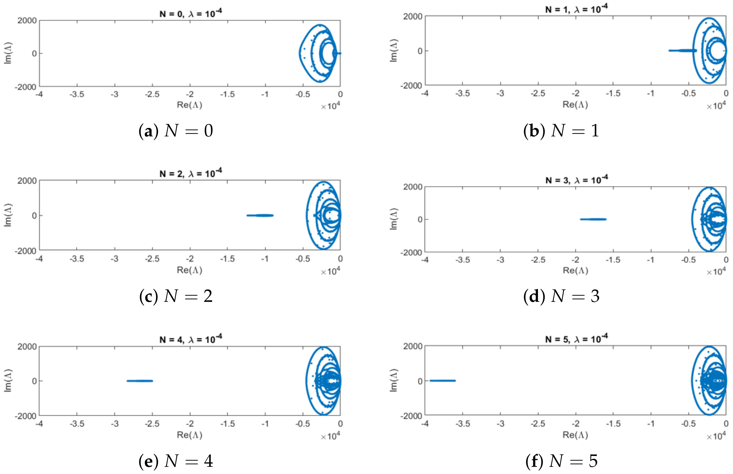
The inner time step δ t is chosen based on the fast eigenvalue cluster of the eigenvalue spectrum of the complete matrix D x U including the stiff source term. We denoted this eigenvalue as Λ m a x and have observed its behavior using different cases in Figure 3 and Figure 4. As mentioned before, a stable inner time step size δ t is later chosen as the inverse of the fastest eigenvalue, i.e., δ t = 1 Λ m a x .
Based on the numerical computation of the spectral analysis, we propose an approximate formula which calculates Λ m a x directly for the dam break test case using the FORCE scheme:
Λ m a x = 1 δ t 421 + N 3 3 1 + 0.01 Δ x 1 · 1 N ( N 1 ) 100 + ( N + 1 ) 2 10 · λ ,
where N denotes the number of moments, Δ x denotes the spatial grid size, and λ is the slip length. The formula was obtained using a careful experimental study with varying N = 0 , ,   5 , n x = 100 ,   200 , ,   1000 , and λ = 10 3 , 10 4 , 10 5 , 10 6 , as will be explained below. The complete set of data is given in Table A1, Table A2, Table A3, Table A4 and Table A5 in Appendix C.
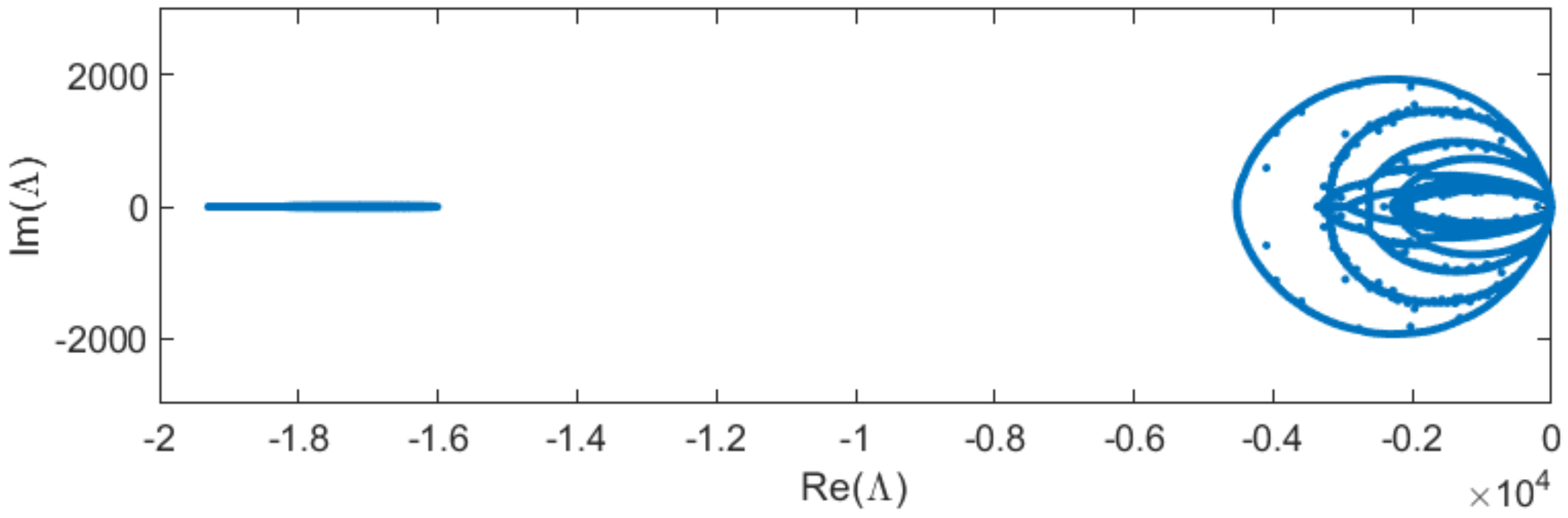
First, we consider the rightmost contribution ( N + 1 ) 2 10 · λ that contains the dependency on λ , compare also Figure 4. 
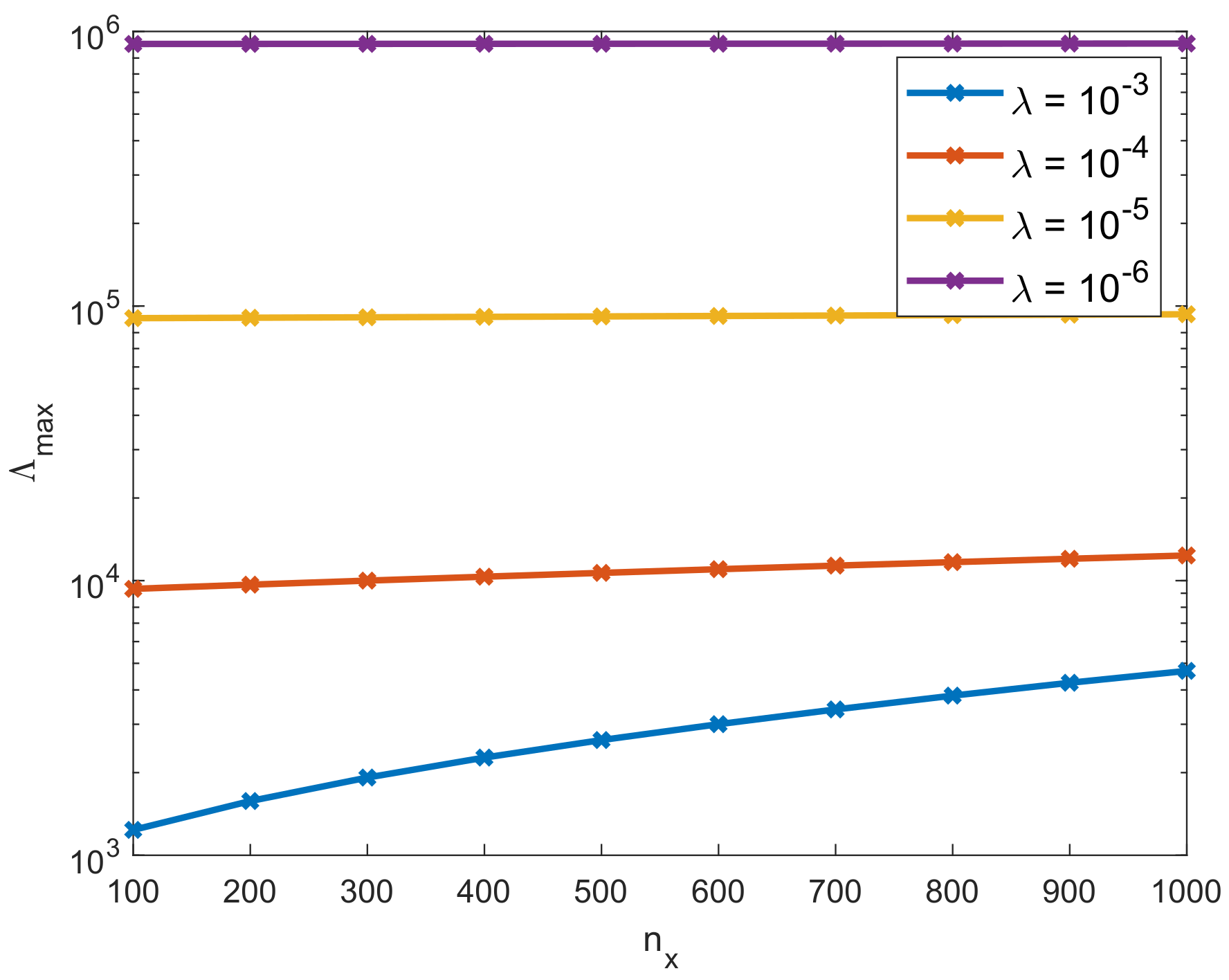
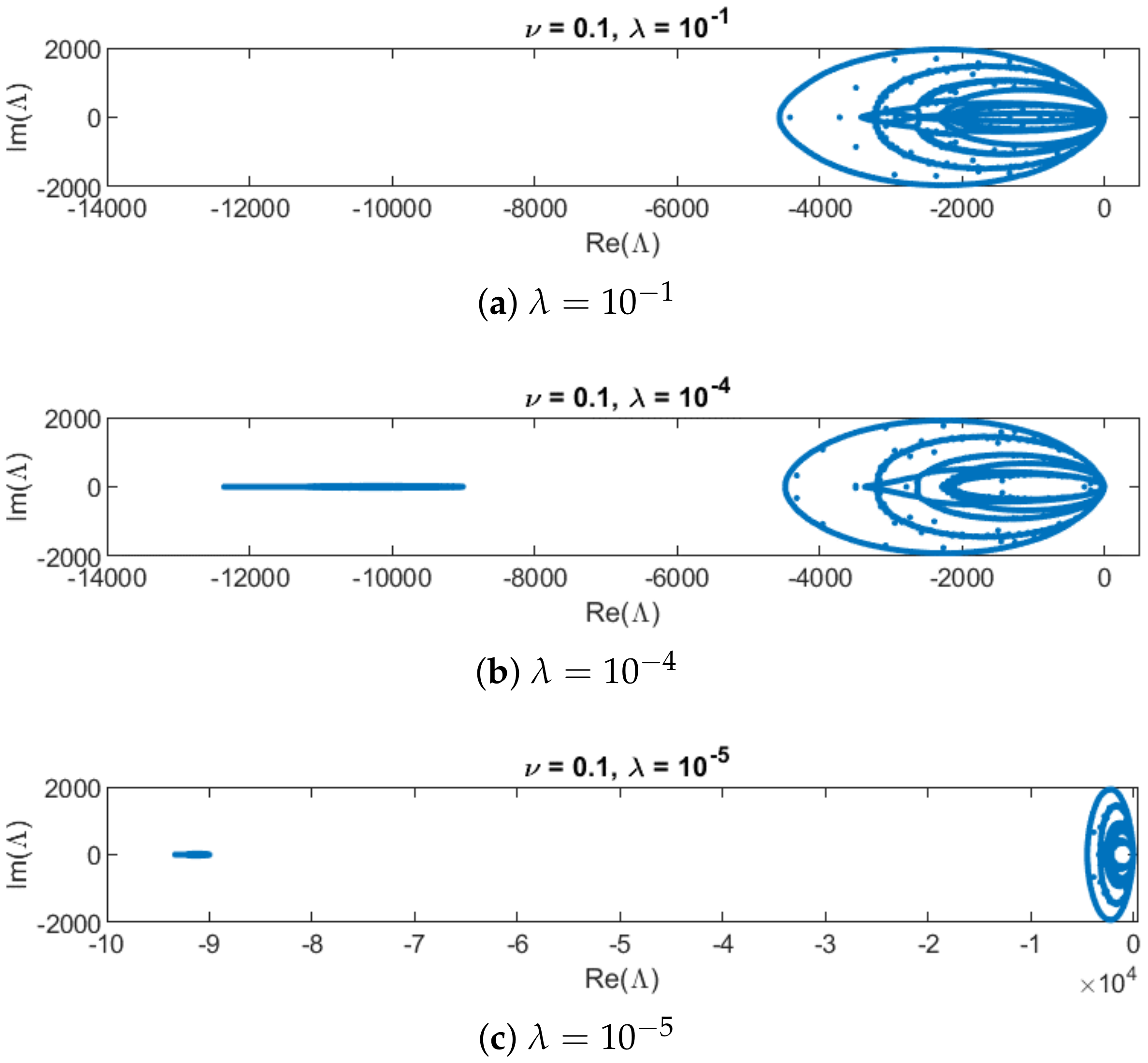
Figure 5 shows the numerically computed Λ m a x for varying slip length λ and varying spatial resolution n x when N = 2 . However, before identifying the contribution of λ to Λ m a x , we first need to split the dependency on λ and n x . In Figure 6, we see that Λ m a x ( N + 1 ) 2 10 · λ is practically independent of the slip length λ , especially for the important case of small λ . The numerically computed values of the eigenvalues Λ m a x can thus be split into two terms, which will be given by Λ m a x = Λ m a x ( N + 1 ) 2 10 · λ + ( N + 1 ) 2 10 · λ , for more details see Table A2. The numerator of the last term can be expressed as ( N + 1 ) 2 according to Table A3. The rightmost contribution in (29) given by ( N + 1 ) 2 10 · λ thus correctly models the dependency on λ .
To study the rest of the formula, we investigate the remaining part Λ m a x ( N + 1 ) 2 10 · λ , and we will validate the model in Equation (29), i.e.,
Λ m a x ( N + 1 ) 2 10 · λ = 421 + N 3 3 1 + 0.01 Δ x 1 · 1 N ( N 1 ) 100 .
In Figure 6, we have observed that this part is independent of the slip length λ for small λ . The following test cases thus use a fixed slip length λ = 10 4 .
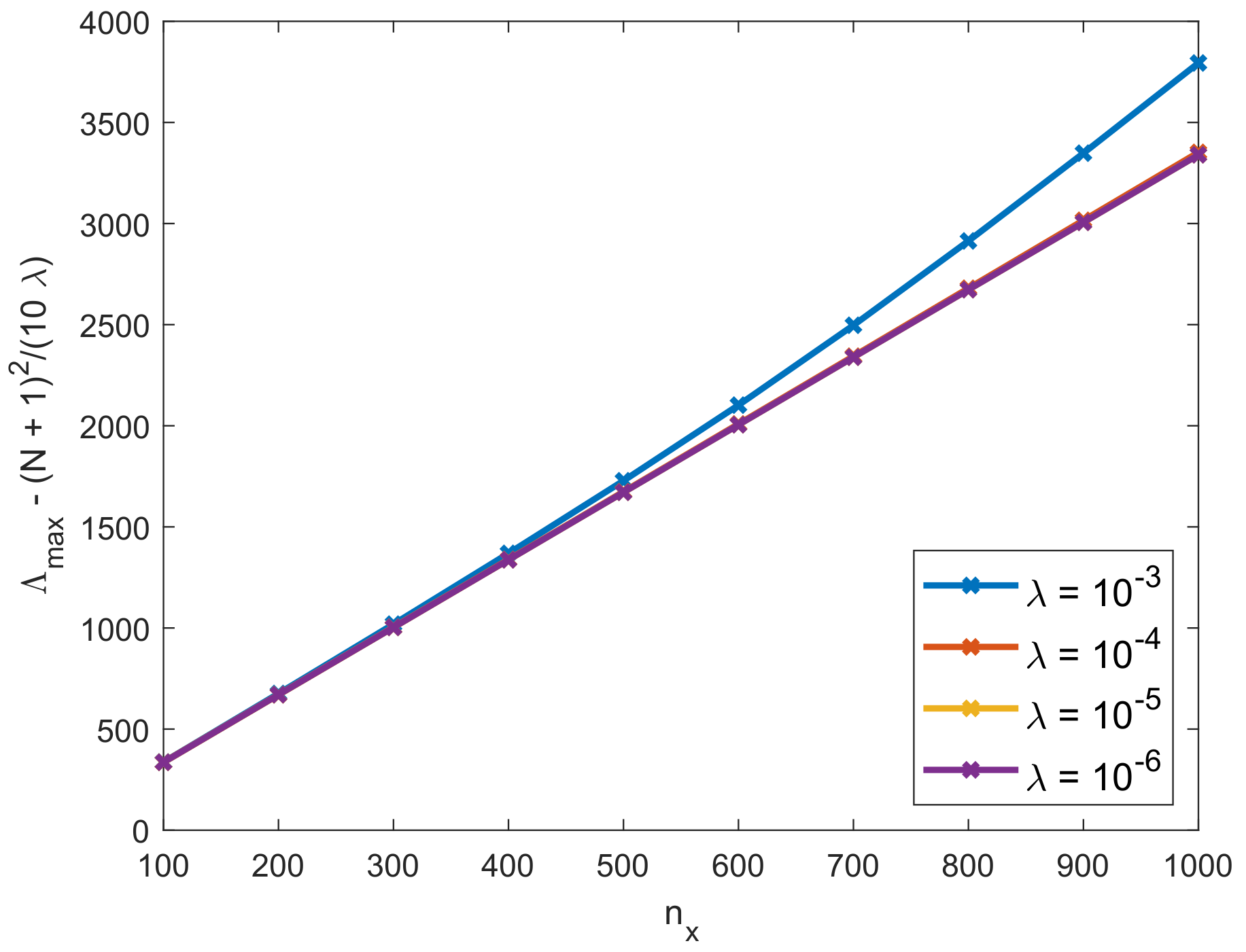
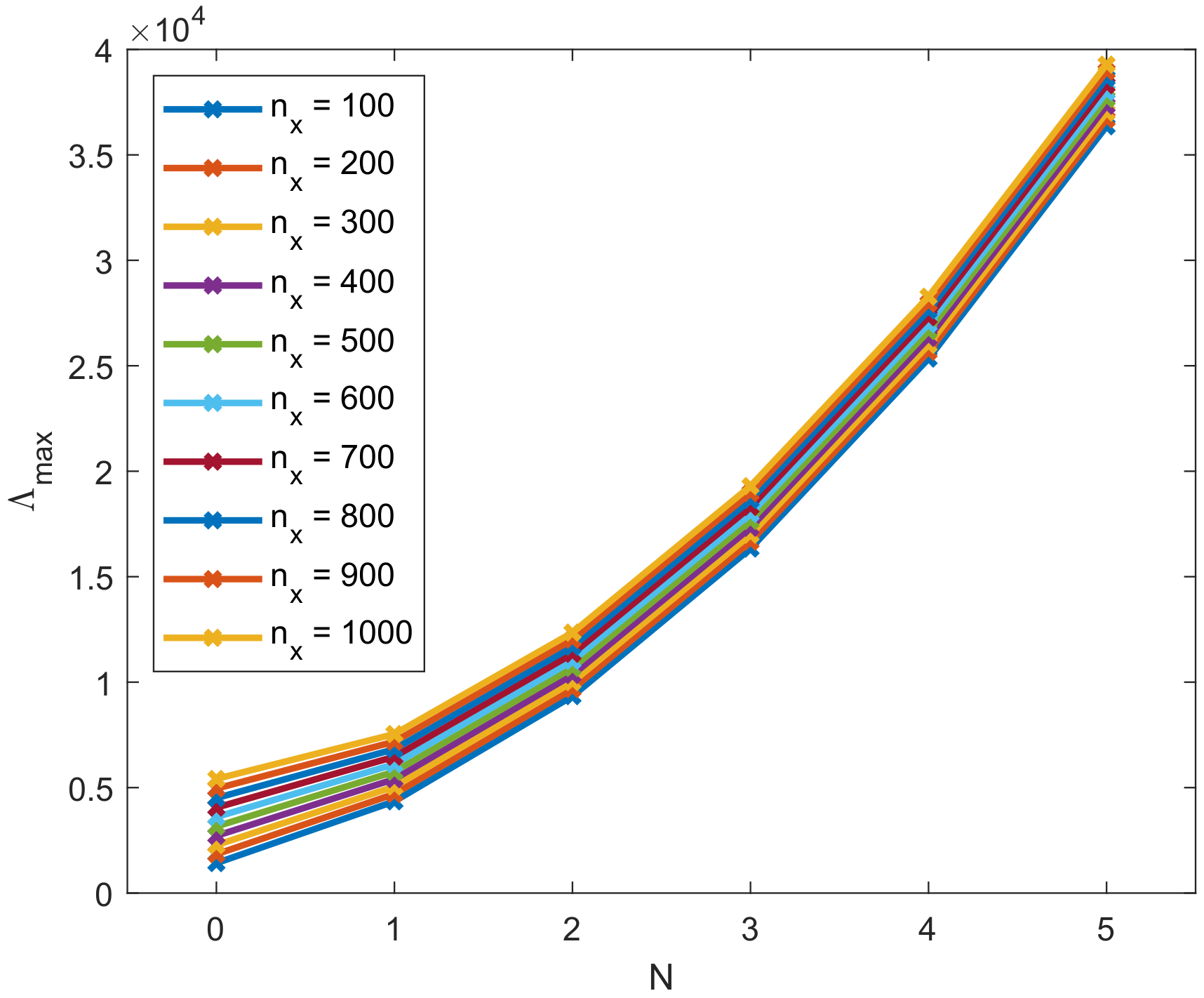
Figure 7 shows the values of Λ m a x for varying N and Δ x . We first focus on a constant n x = 100 to derive an approximation for Λ m a x ( N + 1 ) 2 10 · λ depending only on N and then correct this formula by a factor for different n x 
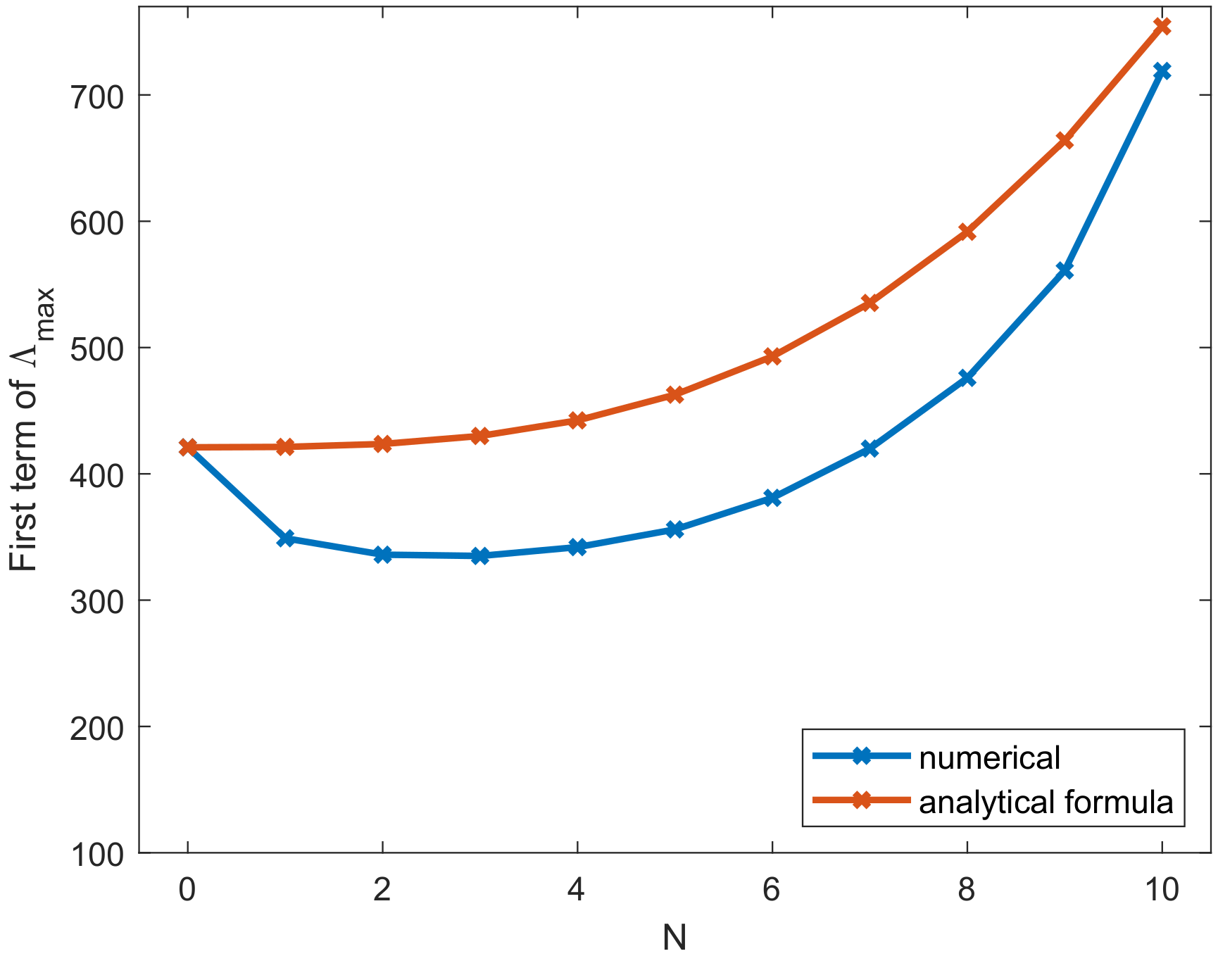
. In order to approximate the values for n x = 100 , we fit a third order polynomial in N. As a constraint, we ensure that the approximated values do not underestimate the numerically obtained values, which would lead to too large values for δ t and stability problems later. Based on that, we obtain the term 421 + N 3 3 , which approximates the dependency of Λ m a x ( N + 1 ) 2 10 · λ on N for constant n x = 100 with increasing accuracy, as seen in Figure 8.
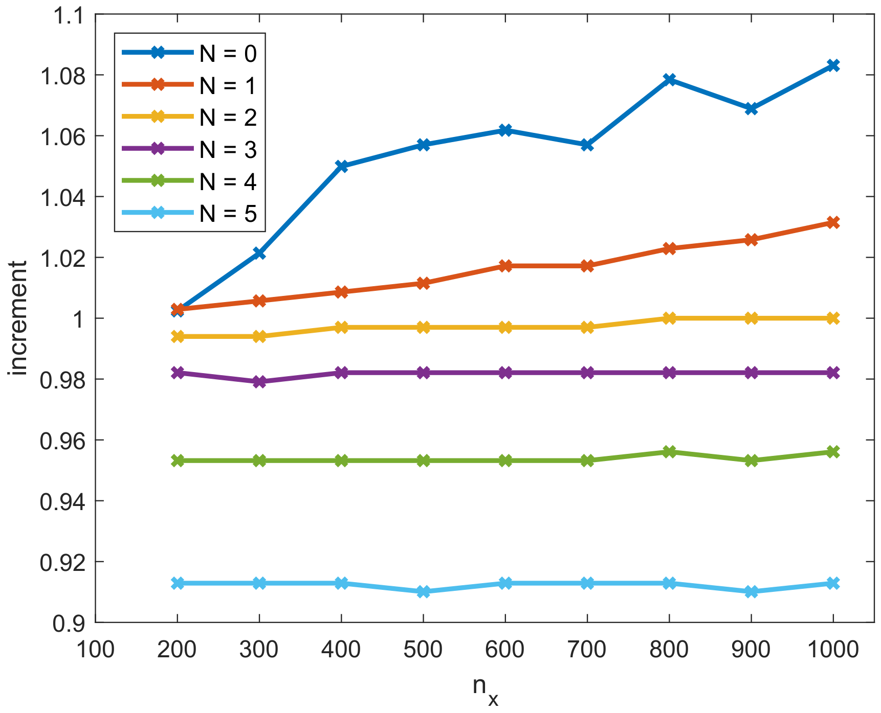
What remains is to correct for different spatial discretizations n x 100 . We do this by using a correction factor, which increments the value obtained for n x = 100 . For maximal accuracy, we allow the correction factor, the so-called increment, to depend on N besides n x . In Figure 9, the numerical value of the increment depending on n x and N is given, based on the numerical computation of the spectrum and the data in Table A4. As expected, the values for small N and n x are close to one, as almost no correction is necessary. For larger values N and n x , a larger correction is necessary. Additionally, the influence of N seems to be larger than the influence of n x . Modeling a small linear dependence on Δ x and a quadratic dependence on N, we obtain 1 + 0.01 Δ x 1 · 1 N ( N 1 ) 100 for the increment, which directly results in Equation (29).
In summary, Equation (29) thus approximates the fastest eigenvalue Λ m a x for the dam break test case and can be used to determine the time step size of the inner integrator by δ t = 1 Λ m a x .
For the smooth periodic wave test case, a similar procedure results in the following formula for the fastest eigenvalue Λ m a x . We leave out the details and give the final result here.
Λ m a x = 1 δ t 364 + N 3 3 1 + 0.01 Δ x 1 · 1 N ( N 1 ) 100 + ( N + 1 ) 2 10 · λ .
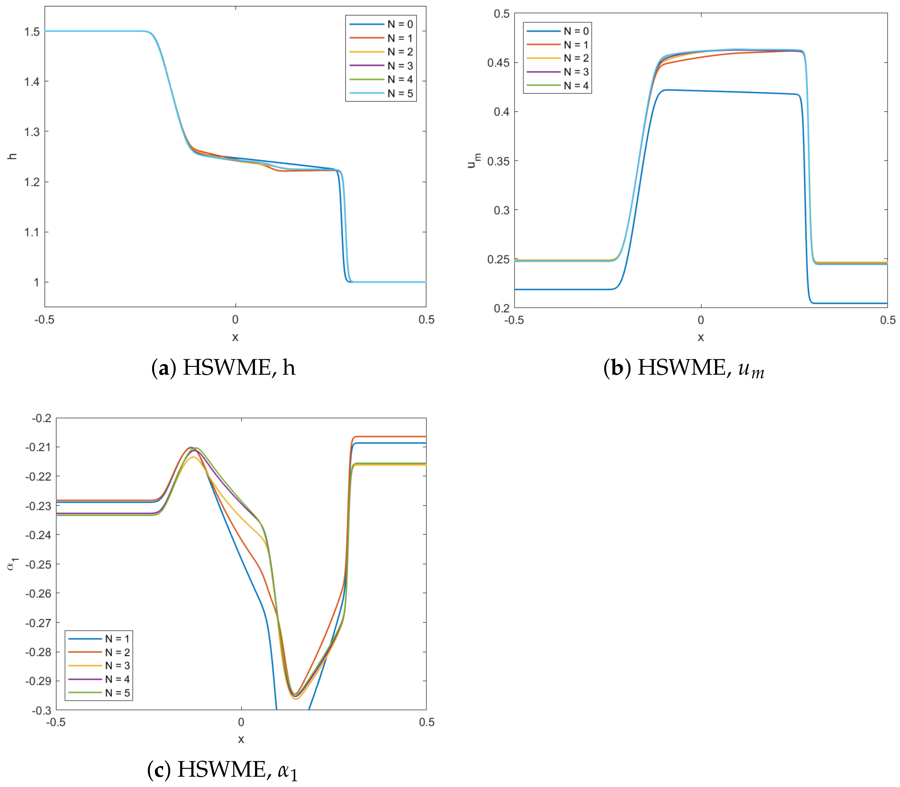
Note that the dependence of the fastest eigenvalue on N, Δ x , and λ is exactly the same for the dam break test case and for the smooth periodic wave test case. Only the leading term changes slightly. This is due to the different initial conditions used in the test cases. However, as the hyperbolic shallow water moment models are balance laws including conservation of mass, no new maximal values inside the computational domain are expected during the simulations such that the fastest eigenvalue is not expected to exceed this value.
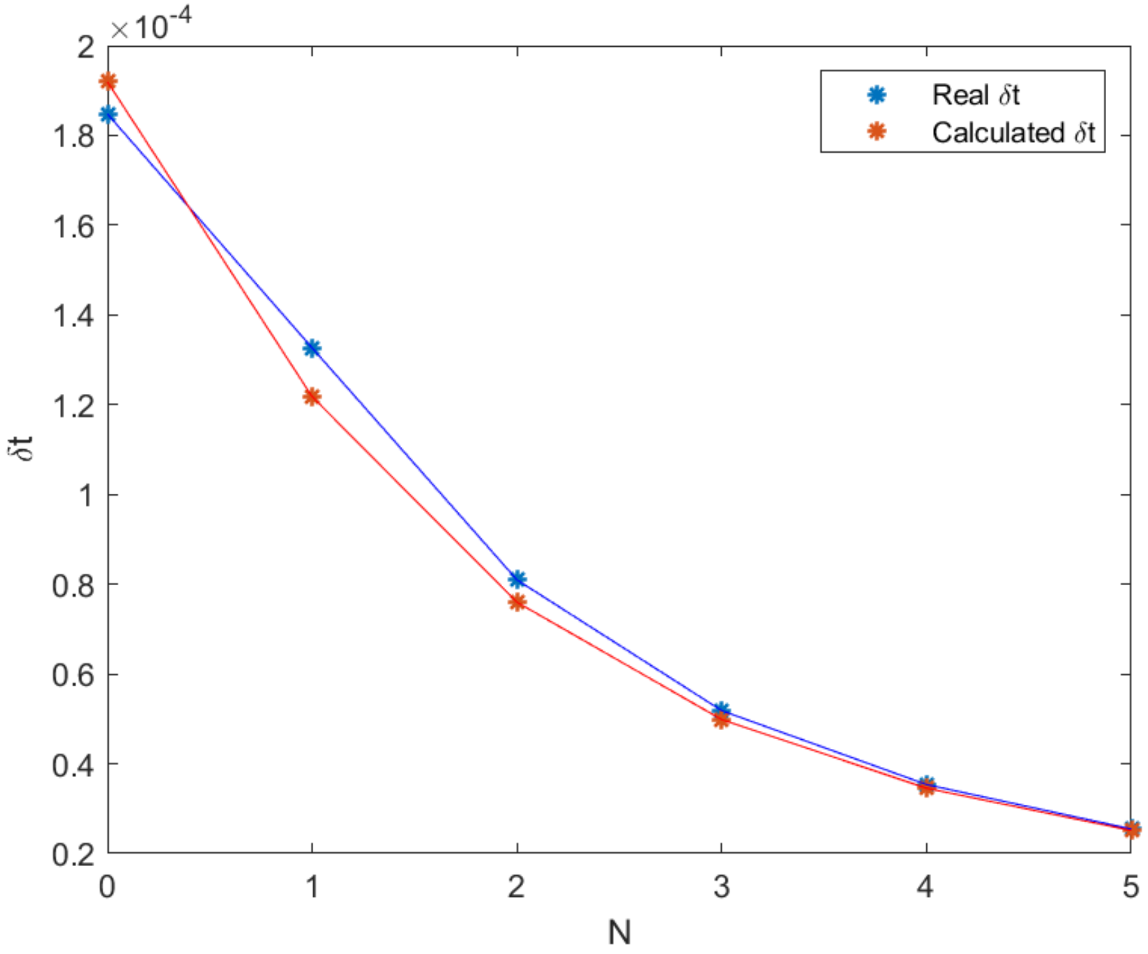
With the numerical results, we also show that the error between the approximated parameter choice for δ t and the stability limit for δ t based on the numerical spectrum, is small, see Table 4 for the dam break test case and Table 10 for the smooth periodic wave. The approximation formulas Equations (29) and (31) are thus effective at computing the inner time step of the PFE method.

4.3.3. Stability Check of PFE Method

In order to check the stability of the PFE method using the previously derived parameters, we consider a typical test case and plot the stability region of the PFE method together with the numerically obtained eigenvalue spectrum. If all eigenvalues lie inside the stability region, the PFE method will result in a stable solution.
According to [10], the stability domain of the PFE method is characterized by
1 + Δ t Δ x K Λ δ t · ( 1 + Λ δ t ) K 1
and this stability condition [10] is satisfied for all eigenvalues Λ that fulfill
Λ D 1 Δ t , 1 Δ t D 1 δ t , 1 δ t δ t Δ t 1 K ,
where D ( c , r ) C denotes the disc with center ( c , 0 ) and radius r in the complex plane.
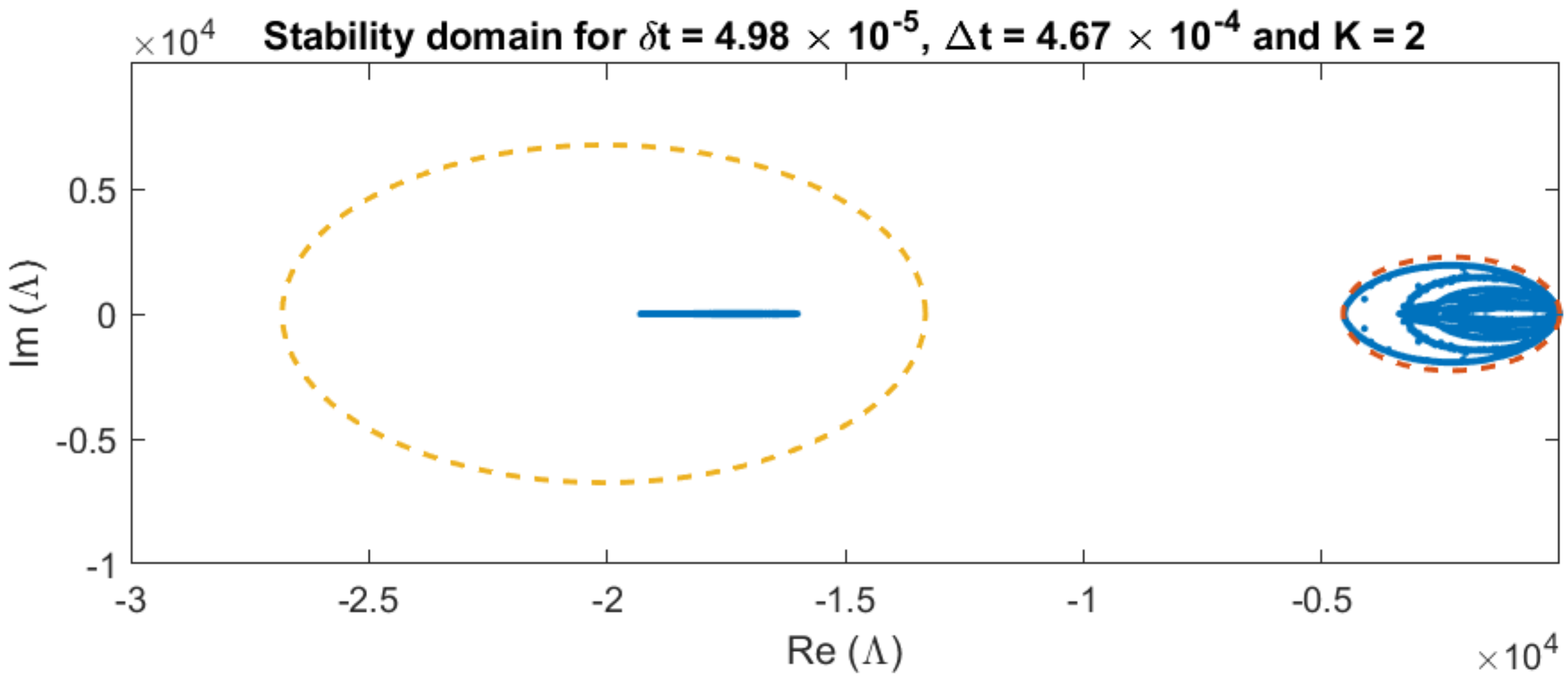
Considering the dam break test case with slip length λ = 10 4 , friction coefficient ν = 0.1 , spatial resolution n x = 1000 and N = 3 moments, the parameters of the PFE method are computed according to the aforementioned stability analysis as δ t = 4.98 × 10 5 and Δ t = 4.67 × 10 4 . Additionally, we use a standard K = 2 . The eigenvalue spectrum of the test case is plotted together with the stability region of the PFE method in Figure 10.
Figure 10 shows that both the fast and the slow eigenvalue clusters lie inside the stability domain, the PFE method with the chosen parameters is thus stable. Comparable results are obtained for the smooth periodic wave test case.

5. Numerical Results

This section contains two numerical experiments taken from [3] to show the applicability and speedup of the PFE method.

5.1. Dam Break Test Case

For the non-smooth dam break test case with discontinuous initial condition, Table 1 shows the standard setup and the initial values from [3]. For this non-stiff setting of λ = 10 1 , Figure 11 shows the result of the dam break problem for height h, velocity u m , and first moment α 1 using the HSWME model for varying N = 0 , , 5 at time t = 0.2 . Figure 11 shows that the model is converging when increasing the number of moments.

5.1.1. Projective Integration Setup for Stiff Test Case

Next, we consider a stiff test setting. The same initial conditions as in Table 1 are used, but the value of the slip length is decreased from λ = 10 1 to λ = 10 4 resulting in a stiff setup. As studied in Section 4, PI is effective in overcoming the severe time step constraint of a standard FE scheme in this case. We will thus apply the PFE scheme and determine suitable parameters first.
For this test case with varying N, constant CFL number C F L 0.7 and Δ x = 0.001 , the outer time step size Δ t is given according to the analysis in Section 4.3.1 as noted in Table 3. Note that Table A1 shows that the maximum eigenvalue for N > 0 is the same.
Stiffness caused by a small λ leads to a very small time step δ t Δ t , which decreases as the value of N increases as seen in Section 4.3.2. Using Equation (29), the values of the inner time step size δ t are evaluated in Table 4. Table 4 also shows the relative error of the inner time step δ t as computed with the approximate Equation (29) compared to the values computed from the full spectrum of the semi-discrete model. Evidently, the error is small and Equation (29) yields an accurate prediction of a stable inner time step size.
Figure 12 shows the comparison of the maximum possible inner time step size δ t obtained from the numerically eigenvalue spectrum with the calculated inner time step size using the formula (29).
In Figure 12, it is observed that for N > 0 the numerically estimated δ t is approximately the same as the exact δ t calculated from the numerically computed eigenvalue spectrum, including a small positive safety margin. The case N = 0 is different, due to the overlap of fast and slow eigenvalue clusters, which are considered in detail in the next subsection. The error is decreasing as N increases, compare Table 4.

5.1.2. Projective Integration Validation

In this section, we compare the results of a FE scheme with small time step size and a PFE scheme as set up above for the stiff dam break test case at t = 0.2 and for ν = 0.1 and λ = 10 4 .
In Figure 13a,b, the height h is shown at time t = 0.2 for both schemes. The HSWME model converges as N increases with increasing accuracy. Notably, the FE and PFE methods give visually the same solution (but yield different runtimes as seen in the next section).
The result for N = 0 differs from other N 0 for h and u m . To understand this behavior we note that the HSWME model for N = 0 is effectively the shallow water model including the standard friction term seen in Equation (10) [3]. As the slip length λ = 10 4 is small, the friction term becomes large. This leads to a fast relaxation of the mean velocity towards zero, which is also visible in Figure 13c,d.
Figure 13e,f plot the first moment which is initially α 1 = 0.25 in our test case and also converges for both the FE and the PFE method.
In all the above cases, we see that the model converges and is accurate compared to Figure 11. Increasing the number of moments also increases the accuracy of the model.
Figure 14 shows the difference between the FE and PFE methods for the dam break test case. For both the water height h and the first moment α 1 , it can be observed that the difference is indeed negligible in smooth regions. Only close to shocks with large gradients, a small difference remains, which is small in relation to the actual solution and the model error [3]. Note that the difference for h increases with N, whereas the difference for α 1 decreases with N as the shock becomes slightly less pronounced, compare Figure 13e.

5.1.3. Runtime

This section focuses on the runtime and speedup of the FE scheme and the PFE scheme. The scheme was implemented in MATLAB without further code optimization, such that the absolute runtime is not relevant but the runtimes can be compared. We thus focus on the speedup. Note that the theoretical speedup S t h for a PFE method with the assumption of neglecting the extrapolation step is in given Equation (25).
In Table 5, the runtime is shown for both the FE and the PFE scheme on a grid using n x = 1000 cells. K denotes the number of inner time steps and S n u m denotes the numerical speedup of the PFE scheme compared to the FE Method. The theoretical speedup S t h as computed from Equation (25) is the maximum possible speedup and thus always larger than the numerical speedup S n u m . Nevertheless, we observe that the PFE scheme leads to a significant speedup with respect to the FE scheme and the numerically obtained values for the speedup are close to the maximum theoretical values.

5.1.4. Spatial Resolution

In this section, more tests are done to illustrate how PI behaves when the spatial resolution is doubled. The left hand side in Figure 15 is computed using a grid with n x = 1000 cells or Δ x = 0.001 whereas the right hand side is computed using a grid with n x = 2000 cells or Δ x = 0.0005 . We see that the solution is already converged on the grid and a refinement of the grid does not lead to a much better resolution of the solution structure.
Table 6 shows the effect of doubling the number of spatial points on the runtime and speedup with respect to a FE scheme. For finer spatial grids, the CFL condition leads to a smaller outer time step size Δ t . The stability restriction imposed by stiffness is thus less severe in relation to the CFL condition. This leads to a smaller speedup of the PFE method compared to Table 5. Additionally, all runtimes increase due to the increase in grid points and the smaller Δ t , by a factor of approximately four, if the same number of inner time steps K was used. However, the smaller spectral gap allows for a smaller K as well, which results in a acceleration of the PFE scheme as well as for the FE scheme.
As the solution already seemed converged for the coarse grid using n x = 1000 grid points, it is possible to employ a fast PFE scheme on the coarse grid without significant loss of spatial accuracy and thereby reduce the runtime.

5.1.5. Varying Stiffness

This section discusses the effect of changes in the stiffness parameter. In Section 4.2, the eigenvalue spectra with different spectral gaps were plotted for different values of λ , see Figure 4.
Choosing suitable values for the PFE parameters for different values of λ according to the analysis in Section 4, the PFE method achieves a significant speedup with respect to the FE method for small values, as seen in Table 7. The speedup is especially large for very small values of λ , due to the large spectral gap and the severe time step constraint of the FE method. We note that the additional overhead of the PFE method including the extrapolation, i.e., the difference between the theoretical speedup S t h and the numerical speedup S n u m is approximately 10 % , pointing to a relatively efficient implementation of the scheme.

5.1.6. Alternative Numerical Scheme

The results above generalize to other spatial discretization schemes. As one example, we show results for the Lax–Friedrichs scheme, see Equation (17). From Figure 16, it can be seen that both schemes converge in the same way, and the accuracy is improved as the number of moments increases.
The runtime and speedup of the PFE scheme with the Lax–Friedrichs spatial discretization employed is shown in Table 8. Comparing with Table 5, it is noticed that the Lax–Friedrichs scheme is faster in comparison to the FORCE scheme. The reason for this is the more involved spatial discretization of the FORCE scheme, see Equation (19).

5.2. Smooth Periodic Wave Test Case

In this section, we present a smooth test case with continuous initial condition taken from [3]. Table 2 in Section 4 shows the standard setup and the initial values from [3].
For the non-stiff setting, Figure 17 shows the result of the smooth periodic wave problem for height h, velocity u m and first moment α 1 using the HSWME for varying N = 0 , , 5 at time t = 0.2 . Figure 17 shows that the model is converging when increasing the number of moments.

5.2.1. Projective Integration Setup for Stiff Test Case

Next, we consider a stiff test setting. The same initial conditions as in Table 2 are used, but the value of the slip length is decreased from λ = 10 1 to λ = 10 4 .
For this test case we use a similar setup as for the previous test case. The maximum outer time step size is now given according to Table 9.
Stiffness caused by a small λ leads to a very small time step δ t Δ t , which decreases as the value of N increases as seen in Section 4.3.2. Using Equation (31), the values of the inner time step size δ t are evaluated according to Table 10.
Similar as for the dam break case, the numerical predictions of the inner time step size δ t according to Table 10 are increasingly accurate in comparison to the exact values.

5.2.2. Projective Integration Validation

In this section, we compare the results of a FE scheme with small time step size and a PFE scheme as set up above for the smooth periodic wave test case, t = 0.2 , ν = 0.1 , and λ = 10 4 .
From Figure 18 at time t = 2 for both schemes, we observe that the model converges with increasing accuracy and both FE and PFE give the same solution. Note again the differences in the results for the N = 0 case.

5.2.3. Runtime

In Table 11, the runtime is shown for both the FE and the PFE scheme on a grid using n x = 1000 cells. For both test cases we observe that the numerically obtained values for the speedup are close but slightly under the maximum theoretical values indicating efficient implementation and significant speedup.

5.2.4. Spatial Resolution

In this section, we illustrate the behavior of the PI method when the spatial resolution is doubled. In Figure 19, we see that the solution is already converged on the grid and a refinement of the grid does not lead to a better accuracy or convergence of the solution.
Table 12 shows the effect of doubling the number of spatial points on the runtime and speedup with respect to a FE scheme. An increase in runtime is also seen here, due to the increase in the number of grid points and the smaller Δ t . The runtime increases by a factor of approximately four, if the same number of inner time steps K was used. Again the smaller spectral gap allows for a smaller K, resulting in an acceleration of both the PFE and the FE scheme scheme.
We note that the results for the dam break test case regarding varying stiffness parameter λ and alternative numerical schemes also hold for the smooth periodic wave test case. They are omitted for conciseness.

6. Conclusions

This paper features the first application of efficient numerical schemes for stiff shallow water moment equations. First, the spectral gap of Hyperbolic Shallow Water Moment Equations is studied numerically. An accurate numerical estimate for the fastest eigenvalue is given and validated for several test cases. This allows to construct explicit stable Projective Integration schemes that overcome the severe time step constraints of the standard Forward Euler scheme. A Projective Forward Euler scheme is applied for a dam break test case and a smooth periodic wave test case and leads to a significant speedup of up to 55 in the stiff regime, while resulting in similar accuracy as the standard Forward Euler scheme. The results of this paper show that Projective Integration schemes are effective in overcoming stiffness and result in fast and accurate numerical solutions.
Further work should focus on the application of higher-order schemes and potential adaptivity in space and time to further accelerate the computation.

Author Contributions

A.A., analysis, software, validation, writing; J.K., methodology, conceptualization, funding acquisition, supervision, writing. All authors have read and agreed to the published version of the manuscript.

Funding

This research has been partially supported by the European Union’s Horizon 2020 research and innovation program under the Marie Sklodowska-Curie grant agreement no. 888596. J. Koellermeier is a postdoctoral fellow in fundamental research of the Research Foundation - Flanders (FWO), funded by FWO grant no. 0880.212.840.

Institutional Review Board Statement

Not applicable.

Informed Consent Statement

Not applicable.

Data Availability Statement

The datasets generated and analysed during this study are available from the corresponding author on reasonable request.

Acknowledgments

The authors would like to acknowledge the financial support of the CogniGron research center and the Ubbo Emmius Funds (University of Groningen).

Conflicts of Interest

The authors declare no conflict of interest.

Appendix A. Second Order System (N = 2)

The shallow water moment equations with two additional moments α 1 and α 2 , where the vertical change in the velocity profile is of second order are given by [3,4]
t h h u m h α 1 h α 2 + x h u m h u m 2 + 1 2 g h 2 + 1 3 h α 1 2 + 1 5 h α 2 2 h u m α 1 + 4 5 h α 1 α 2 h u m α 2 1 3 h α 1 2 + 1 7 h α 2 2 = ν λ 0 u m + α 1 + α 2 3 ( u m + α 1 + α 2 + 4 λ h α 1 ) 5 ( u m + α 1 + α 2 + 12 λ h α 2 ) ,
where, again, g is the gravitation constant, ν is the friction coefficient and λ is the slip length. The right hand side contains the friction terms.
The system matrix for the second order model is defined as [4]
A = 0 1 0 0 g h u m 2 1 3 α 1 2 1 5 α 2 2 2 u m 2 3 α 1 2 5 α 2 2 u m α 1 4 5 α 1 α 2 2 α 1 u m + α 2 3 5 α 1 2 3 α 1 2 2 u m α 2 2 7 α 2 2 2 α 2 1 3 α 1 u m + 3 7 α 2 .
The eigenvalues of the above system matrix have the form a i = u m + c i g h , with c i being the i t h root of the following polynomial
χ ( c ) = c 4 10 7 α 2 c 3 1 + 6 35 α 2 2 + 6 5 α 1 2 c 2 + 22 35 α 2 3 6 35 α 2 α 1 2 + 10 7 α 2 c 1 35 α 2 4 6 35 α 2 2 α 1 2 3 7 α 2 2 + 1 5 α 1 4 + 1 5 α 1 2 .
Calculating the roots for different parameter values of α 1 and α 2 can result in complex values, which indicates a lack of hyperbolicity [4]. A hyperbolic matrix A H is obtained by setting α 2 = 2 in Equation (A2).

Appendix B. Eigenvalues for Larger Moment Models

Table A1 shows the real and distinct eigenvalues of the HSWME system matrix A H (7) for N = 0 , , 5 according to [3].
Table A1. Eigenvalues of HSWME system matrix A H (7) for N = 0 , , 5 .
N012345
EV1 u m + g h u m + g h + α 1 2 u m + g h + α 1 2 u m + g h + α 1 2 u m + g h + α 1 2 u m + g h + α 1 2
EV2 u m g h u m g h α 1 2 u m g h α 1 2 u m g h α 1 2 u m g h α 1 2 u m g h α 1 2
EV3- u m u m + 1 5 α 1 u m + 3 7 α 1 u m + ( 1 3 2 3 7 ) α 1 u m + 15 2 15 33 α 1
EV4-- u m 1 5 α 1 u m 3 7 α 1 u m ( 1 3 2 3 7 ) α 1 u m 15 2 15 33 α 1
EV5--- u m u m + ( 1 3 + 2 3 7 ) α 1 u m + 15 + 2 15 33 α 1
EV6---- u m ( 1 3 + 2 3 7 ) α 1 u m 15 + 2 15 33 α 1
EV7----- u m

Appendix C. Eigenvalue Data

This section contains the data used to derive the analytical formula in Section 4.3.2.
Table A2 and Table A3 show the fastest eigenvalues Λ m a x among the numerically computed eigenvalues of the semi-discrete system (21) for varying λ , n x , and N = 0 , , 5 .
Table A2. Fastest eigenvalue Λ m a x as λ decreases for different n x , λ , and constant N = 2 . For a visualization, see Figure 5.
n x λ = 10 3 λ = 10 4 λ = 10 5 λ = 10 6
100 1237 = 337 + 900 9336 = 336 + 9 × 10 3 90,336 = 336 + 9 × 10 4 900,336 = 336 + 9 × 10 5
200 1576 = 676 + 900 9670 = 670 + 9 × 10 3 90,670 = 670 + 9 × 10 4 900,670 = 670 + 9 × 10 5
300 1919 = 1019 + 900 10,004 = 1004 + 9 × 10 3 91,003 = 1003 + 9 × 10 4 901,003 = 1003 + 9 × 10 5
400 2269 = 1369 + 900 10,339 = 1339 + 9 × 10 3 91,337 = 1337 + 9 × 10 4 901,337 = 1337 + 9 × 10 5
500 2628 = 1728 + 900 10,674 = 1647 + 9 × 10 3 91,671 = 1671 + 9 × 10 4 901,671 = 1671 + 9 × 10 5
600 3002 = 2102 + 900 11,009 = 2009 + 9 × 10 3 92,005 = 2005 + 9 × 10 4 902,005 = 2005 + 9 × 10 5
700 3397 = 2497 + 900 11,344 = 2344 + 9 × 10 3 92,339 = 2339 + 9 × 10 4 902,339 = 2339 + 9 × 10 5
800 3814 = 2914 + 900 11,680 = 2680 + 9 × 10 3 92,673 = 2673 + 9 × 10 4 902,673 = 2673 + 9 × 10 5
900 4248 = 3348 + 900 12,016 = 3016 + 9 × 10 3 93,006 = 3006 + 9 × 10 4 903,006 = 3006 + 9 × 10 5
1000 4694 = 3794 + 900 12,352 = 3352 + 9 × 10 3 93,340 = 3340 + 9 × 10 4 903,340 = 3340 + 9 × 10 5
Table A3. Fastest eigenvalue Λ m a x for different n x , N, and constant λ = 10 4 . For a visualization, see Figure 7.
n x N = 0 N = 1 N = 2 N = 3 N = 4 N = 5
10014214349933616,33525,34236,356
20018434699967016,66425,66836,681
3002273505010,00416,99225,99437,006
4002715540210,33917,32126,32037,331
5003160575510,67417,65026,64637,655
10005412754012,35219,29528,27839,279
Table A4. First term of eigenvalue Λ m a x for different N and n x , and constant λ = 10 4 . For a visualization, see Figure 9.
n x N = 0 incr N = 1 incr N = 2 incr N = 3 incr N = 4 incr N = 5 incr
100421-349-336-335-342-356-
2008431.006991.006700.996640.986680.956810.91
30012731.0210501.0110040.999920.989940.9510060.91
40017151.0514021.0113391.0013210.9813200.9513310.91
50021601.0617551.0116741.0016500.9816460.9516550.91
100044121.0835401.0333521.0032950.9832780.9532790.91
Table A5. First term of the eigenvalue Λ m a x for different N, constant n x = 100 , and λ = 10 4 . For a visualization, see Figure 8.
N012345678910
Λ m a x 421349336335342356381420476561719

References

  1. Christen, M.; Kowalski, J.; Bartelt, P. RAMMS: Numerical simulation of dense snow avalanches in three-dimensional terrain. Cold Reg. Sci. Technol. 2010, 63, 1–14. [Google Scholar] [CrossRef] [Green Version]
  2. Miglio, E.; Quarteroni, A.; Saleri, F. Finite element approximation of quasi-3d shallow water equations. Comput. Methods Appl. Mech. Eng. 1999, 174, 355–369. [Google Scholar] [CrossRef]
  3. Koellermeier, J.; Rominger, M. Analysis and numerical simulation of hyperbolic shallow water moment equations. Commun. Comput. Phys. 2019, 28, 1038–1084. [Google Scholar]
  4. Kowalski, J.; Torrilhon, M. Moment approximations and model cascades for shallow flow. Commun. Comput. Phys. 2019, 25, 669–702. [Google Scholar] [CrossRef] [Green Version]
  5. Kern, M.A.; Bartelt, P.A.; Sovilla, B. Velocity profile inversion in dense avalanche flow. Ann. Glaciol. 2010, 51, 27–31. [Google Scholar] [CrossRef] [Green Version]
  6. Huang, Q.; Koellermeier, J.; Yong, W.-A. Equilibrium stability analysis of hyperbolic shallow water moment equations. Math. Method. Appl. Sci. 2022, in press. [Google Scholar] [CrossRef]
  7. Garres-Díaz, J.; de Luna, T.M.; Castro, M.J.; Koellermeier, J. Shallow water moment models for bedload transport problems. Commun. Comput. Phys. 2021, 11, 435–467. [Google Scholar]
  8. Gear, C.; Kevrekidis, I. Projective methods for stiff differential equations: Problems with gaps in their eigenvalue spectrum. SIAM J. Sci. Comput. 2001, 24, 1091–1106. [Google Scholar] [CrossRef] [Green Version]
  9. Melis, W.; Rey, T.; Samaey, G. Projective integration for nonlinear BGK kinetic equations. In Finite Volumes for Complex Applications VIII—Hyperbolic, Elliptic and Parabolic Problems; Springer Proceedings in Mathematics & Statistics; Cancès, C., Omnes, P., Eds.; Springer: Cham, Switzerland, 2017; Volume 200, pp. 145–153. [Google Scholar]
  10. Koellermeier, J.; Samaey, G. Projective integration schemes for hyperbolic moment equations. Kinet. Relat. Model. 2021, 14, 353–387. [Google Scholar] [CrossRef]
  11. Melis, W.; Rey, T.; Samaey, G. Projective and telescopic projective integration for the nonlinear BGK and Boltzmann equations. SMAI J. Comput. Math. 2017, 5, 53–88. [Google Scholar] [CrossRef] [Green Version]
  12. Castro, M.J.; LeFloch, P.G.; Munoz-Ruiz, M.L.; Pares, C. Why many theories of shock waves are necessary: Convergence error in formally path-consistent schemes. J. Comput. Phys. 2008, 227, 8107–8129. [Google Scholar] [CrossRef] [Green Version]
  13. Castro, M.; Koellermeier, J. High-order non-conservative simulation of hyperbolic moment models in partially-conservative form. East Asian J. Appl. Math. 2021, 11, 435–467. [Google Scholar] [CrossRef]
  14. Madroñal, C. Numerical methods for nonconservative hyperbolic systems: A theoretical framework. SIAM J. Numer. Anal. 2006, 44, 300–321. [Google Scholar]
  15. LeVeque, R.J. Finite Volume Methods for Hyperbolic Problems; Cambridge Texts in Applied Mathematics; Cambridge University Press: Cambridge, UK, 2002. [Google Scholar]
  16. Harten, A.; Lax, P.D.; Leer, B.V. On upstream differencing and Godunov-type schemes for hyperbolic conservation laws. SIAM Rev. 1983, 25, 35–61. [Google Scholar] [CrossRef]
  17. Castro, M.; de Luna, T.M.; Madroñal, C. Well-balanced schemes and path-conservative numerical methods. Handb. Numer. Anal. 2016, 18, 131–175. [Google Scholar]
  18. Canestrelli, A.; Siviglia, A.; Dumbser, M.; Toro, E.F. Well-balanced high-order centred schemes for non-conservative hyperbolic systems. Applications to shallow water equations with fixed and mobile bed. Adv. Water Resour. 2009, 32, 834–844. [Google Scholar] [CrossRef]
  19. Castro, M.; Fernández-Nieto, E. A class of computationally fast first order finite volume solvers: PVM methods. SIAM J. Sci. Comput. 2012, 34, A2173–A2196. [Google Scholar] [CrossRef] [Green Version]
Figure 1. Eigenvalue Spectrum with a large spectral gap of eigenvalues ( Λ ).
Axioms 11 00235 g001
Figure 2. Projective integration: an explicit method is applied over small time steps (black dots) to stably integrate fast modes, then the solution is extrapolated using a much larger time step (dashed lines), modified from [9,11].
Axioms 11 00235 g002
Figure 3. Eigenvalue spectrum with increasing spectral gap for dam-break case with varying N and fixed ν = 0.1 , λ = 10 4 .
Axioms 11 00235 g003
Figure 4. Eigenvalue spectrum, with increasing spectral gap for dam-break case with decreasing λ and fixed N = 2 , ν = 0.1 .
Axioms 11 00235 g004
Figure 5. Fastest eigenvalue Λ m a x as λ decreases for different n x and constant N = 2 . For the data, see Table A2.
Axioms 11 00235 g005
Figure 6. Fastest eigenvalue Λ m a x excluding the last part of the analytical formula (29) Λ m a x ( N + 1 ) 2 10 · λ as λ decreases for different n x and constant N = 2 . For the data, see Table A2.
Axioms 11 00235 g006
Figure 7. Fastest eigenvalue Λ m a x for different n x , N and constant λ = 10 4 . For the data, see Table A3.
Axioms 11 00235 g007
Figure 8. Approximation of Λ m a x ( N + 1 ) 2 10 · λ for different N, constant n x = 100 and λ = 10 4 both calculated numerically (blue) and by using the analytical formula 421 + N 3 3 (red). For the data, see Table A5.
Axioms 11 00235 g008
Figure 9. Increment factor of middle term of the analytical formula (29) as n x increases for different N and constant λ = 10 4 . For the data, see Table A4.
Axioms 11 00235 g009
Figure 10. Stability domain of PFE method (yellow dashed for inner integrator, red dashed for outer integrator) for δ t = 4.98 × 10 5 , Δ t = 4.67 × 10 4 and K = 2 together with numerical eigenvalue spectrum (blue dots) for slip length λ = 10 4 , friction coefficient ν = 0.1 , spatial resolution n x = 1000 and N = 3 moments for dam break test case.
Axioms 11 00235 g010
Figure 11. Standard dam break test case with standard parameters [3] for varying N at t = 0.2 shows the convergence of the HSWME model.
Axioms 11 00235 g011
Figure 12. Inner time step size δ t computed using numerical eigenvalue spectrum (real, blue) and formula (29) (calculated, red) depending on different number of moments N shows good agreement.
Axioms 11 00235 g012
Figure 13. Dam break test case using FE (a,c,e) and PFE (b,d,f) schemes, for height h (a,b), mean velocity u m (c,d), and first moment α 1 (e,f), for varying N and constant ν = 0.1 and λ = 10 4 shows visibly the same accuracy for the PFE method.
Axioms 11 00235 g013
Figure 14. Dam break test case difference between FE and PFE schemes, for height h (a) and first moment α 1 (b), for varying N and constant ν = 0.1 and λ = 10 4 shows that the PFE method is the same in smooth regions and exhibits small differences in regions of large gradients as the FE method has a larger error there.
Axioms 11 00235 g014
Figure 15. Dam break test case water height using PFE scheme for different N and two different grids using n x = 1000 (a) and n x = 2000 (b) for constant λ = 10 4 shows that the solution is converged.
Axioms 11 00235 g015
Figure 16. Dam break test case water height using PFE scheme for different N. FORCE discretization (a) and Lax–Friedrichs discretization (b) for constant n x = 1000 and λ = 10 4 shows the same numerical solution.
Axioms 11 00235 g016
Figure 17. Standard smooth periodic test case with standard parameters [3] for varying N at t = 0.2 shows the convergence of the HSWME model.
Axioms 11 00235 g017
Figure 18. Periodic wave test case using FE (a,c,e), and PFE (b,d,f), for height h (a,b), mean velocity u m (c,d), and first moment α 1 (e,f), for varying N and constant ν = 0.1 and λ = 10 4 shows visibly the same accuracy for the PFE method with respect to the FE method.
Axioms 11 00235 g018
Figure 19. Smooth periodic wave test case water height using PFE scheme for different N and two different n x = 1000 (b) and n x = 2000 (a) for constant λ = 10 4 shows that the solution is converged.
Axioms 11 00235 g019
Table 1. Simulation setup for dam break test case.
friction coefficient ν = 0.1
slip length λ = 0.1
spatial domain x [ 0.5 , 0.5 ]
spatial resolution n x = 1000
initial height h ( x ) = 1.5 if x 0 1 if x > 0
initial velocity u ( 0 , x , ζ ) = 0.25 ζ
first moment α 1 = 0.25
CFL number 0.7
numerical scheme F O R C E scheme
Table 2. Simulation setup for smooth periodic wave test case.
friction coefficient ν = 0.1
slip length λ = 0.1
temporal domain t [ 0 , 2 ]
spatial domainperiodic x = [ 1 , 1 ]
spatial resolution n x = 1000
initial height h ( x ) = 1 + exp ( 3 cos ( π ( x + 0.5 ) ) ) / exp ( 4 )
initial velocity u ( 0 , x , ζ ) = 0.25 ζ
first moment α 1 = 0.25
CFL number 0.7
numerical scheme F O R C E scheme
Table 3. Maximum stable outer time step size Δ t for varying N, constant CFL number C F L 0.7 and Δ x = 0.001 for dam break test case.
N Δ t
00.000474
1,2,3,4,50.000467
Table 4. Inner time step size δ t and relative δ t error for varying N, constant CFL number C F L 0.7 and Δ x = 0.001 .
N δ t δ t Error
00.000192−3.7 %
10.0001228.9 %
20.0000766.5 %
30.0000504.0 %
40.0000342.3 %
50.0000251.3 %
Table 5. Dam break test case runtime (in sec) using FE and PFE schemes and speedup of PFE method for different N and constant n x = 1000 , λ = 10 4 shows significant speedup close to the theoretical prediction.
NFEPFEK S num S th
08711.181.24
1191011.901.92
2361312.713.07
3592022.973.12
4962224.364.50
51453234.534.64
Table 6. Dam break test case runtime and speedup using FE and PFE schemes for different N and constant n x = 2000 , λ = 10 4 shows significant speedup close to the theoretical prediction.
NFEPFEK S num S th
0282611.081.12
1543911.381.45
2894711.892.02
31395312.622.81
42128722.422.55
53119623.223.38
Table 7. Dam break test case runtime and speed using FE and PFE schemes for different λ and constant n x = 1000 and N = 2 shows increasing speedup close to the theoretical prediction.
λ FEPFEK S num S th
10 2 12.71310.950.99
10 3 151311.121.18
10 4 361312.713.07
10 5 2723448.008.79
10 6 263948654.9860.28
Table 8. Dam break test case runtime and speedup using FE and PFE schemes with Lax–Friedrichs discretization for different N and constant n x = 1000 and λ = 10 4 shows significant speedup close to the theoretical prediction.
NFEPFEK S num S th
084.611.731.78
119812.372.45
2331422.352.41
3531623.313.50
4812333.523.68
51192534.764.97
Table 9. Maximum stable time step size Δ t for varying N, constant CFL number C F L 0.7 and Δ x = 0.001 for smooth periodic wave test case for non-stiff conditions.
N Δ t
00.000493
1,2,3,4,50.000484
Table 10. Inner time step size δ t and relative δ t error for varying N, constant CFL number C F L 0.7 and Δ x = 0.001 .
N δ t δ t Error
00.000215−2.1%
10.0001317.1%
20.0000795.2%
30.0000513.2%
40.0000351.9%
50.0000251.1%
Table 11. Smooth periodic wave test case runtime (in sec) using FE and PFE schemes and speedup of PFE method for different N and constant n x = 1000 , λ = 10 4 shows significant speedup close to the theoretical prediction.
NFEPFEK S num S th
013111611.131.14
132017411.831.85
263632221.972.03
3108736522.983.15
4174153033.283.44
5271258334.654.76
Table 12. Smooth periodic wave test case runtime and speedup using FE and PFE schemes for different N and constant n x = 2000 , λ = 10 4 shows significant speedup close to the theoretical prediction.
NFEPFEK S num S th
080540012.012.04
1174465312.732.73
2283074713.793.92
3476586715.495.57
47250144325.025.13
510,909162726.706.87
Publisher’s Note: MDPI stays neutral with regard to jurisdictional claims in published maps and institutional affiliations.

