
The Possibility of Combining and Implementing Deep Neural Network Compression Methods

 ,
,  ,
,  and
and 
Abstract
:1. Introduction
- Storing capacities: DNN models use a large number of parameters to achieve a high level of accuracy. Storing all of these parameters requires a large amount of memory. For these reasons, DNN model compression leads to reductions in size and enables their application on resource-constrained devices (RC devices).
- The complexity of calculation: While being executed, DNN models require a great number of floating-point operations per second (FLOPs). RC devices cannot achieve the number of operations required for the application of contemporary models. For that very reason, it is possible to apply compression techniques that reduce the number of calculations while using the model.
- Execution in real-time: Contemporary DNN models require a lot of time for training and execution as well, which reduces their usability for solving the problems that require data processing in real-time. Compressing a model enables us to not only reduce the calculation but also the model calculation time, meaning it is possible to apply the model when processing data in real-time.
- Privacy: If it is not possible to apply a model on an RC device, data have to be transferred via a network to a server capable of running the original model. During this data transfer process to such a server, the possibility of data protection issues and abuse increases. The application of DNN models directly on RC devices eliminates the possibility of such attacks.
- Energy consumption: RC device consumption is primarily determined by the access to the memory. For devices constructed using the 45 nm CMOS technology, a 32-bit collector consumes about 0.9 pJ of energy. That very same technology consumes 5 pJ of energy to access 32-bit data in SRAM and 640 pJ to access 32-bit data in DRAM. Contemporary DNN models cannot be fully stored in a device’s cache memory; for this reason, their execution requires multiple access to DRAM, and simultaneously also a greater consumption of electrical energy. The compression of a DNN model leads to a decrease in energy consumption during its application and prolongs the lifecycle of battery-charged IoT devices [15].
2. Related Works
3. Experimental Testing and Results
- The ImageNet is far too large a dataset to be processed by computational resources provided for this research. The Kaggle platform provides each user of the website a total of 30 free-of-charge hours to train a model on NVIDIA TESLA P100 GPU every week. Simultaneously, one training session (committing one Kaggle kernel) must not run for more than twelve hours. Due to these limitations, the training of a model on the ImageNet dataset is almost impossible.
- In practice, problems with far fewer classes appear more frequently, where a quite specific issue should be solved.
- Using a subset of the ImageNet dataset would require additional work for selecting appropriate subset classes that are easy to train initial models on but still challenging enough to prevent it from differentiating the classes based on some simple feature, such as the most widespread image color.
- The initial (base) model trained on the selected dataset needs to have high enough accuracy so that all degradation of accuracy after model compression can be addressed to the applied compression method.
- The dataset is of a far smaller size, which on its part results in shorter model training.
- The images are preprocessed using Macenko’s color normalization method [40], so there is no need for additional processing.
- Simple models (ResNet18 and ResNet50) generate good results (about 90% accuracy on the validation set) after having been trained on this dataset without additional data processing, so more attention can be paid to the compression techniques themselves.
3.1. Dataset and Subsets
- This is a set of 100,000 non-overlapping segments of the images derived from the histological images of colorectal cancer and the normal human tissue colored using hematoxylin and eosin (H&E).
- All the images are the size of 224 × 224 pixels (px) on the scale of 0.5 microns per pixel. The colors of all the images are normalized using Macenko’s method [40].
- The following tissue classes can be seen in the images: adipose (ADI), background (BACK), debris (DEB), lymphocytes (LYM), mucus (MUC), smooth muscle (MUS), normal colon mucosa (NORM), cancer-associated stroma (STR), and colorectal adenocarcinoma epithelium (TUM).
- The images were selected manually from the N = 86 H&E-colored parts of the human cancerogenic tissue using the formalin-fixed paraffin-embedded (FFPE) formalin obtained from the NCT Biobank (National Center for Tumor Diseases, Heidelberg, Germany) and the pathology archive of the UMM (University Medical Center Mannheim, Mannheim, Germany). The tissue samples contained CRC primary tumor samples, as well as tumor tissue, from the CRC metastases in the liver. The normal tissue classes were augmented with the non-tumor samples to increase variability.
- This is a set of 7180 segments of the images obtained from a total of 50 patients with colorectal adenocarcinoma.
- There is no overlapping in-between the patients used to generate this set and the patients used to generate the NCT-CRC-HE-100K set.
- This set can be used as a validation set for the models trained on a larger set (NCT-CRC-HE-100K). As in the first dataset, the image segments are the size of 224 × 224 px with a scale of 0.5 microns per pixel. All the samples were obtained from the NCT Tissue Bank.
- This is a different version of the NCT-CRC-HE-100K dataset.
- This set contains 100,000 image segments of the nine tissue classes with a scale of 0.5 microns per pixel.
- The same was created based upon the same data as the NCT-CRC-HE-100K set but deprived of image color normalization. For that reason, the intensity of the coloring and the color itself vary from one image to the next. Although this set was generated from the same data as NCT-CRC-HE-100K, the image segments are not completely the same, since the selection of non-overlapping segments is a stochastic process.
3.2. Base Model
- ResNet networks are a very popular solution to solving diverse issues;
- ResNet18 is the simplest model generating quite acceptable results on a selected dataset (about 90% accuracy), without any additional input data processing (except for the already performed color normalization). This is a very important fact enabling us to compare the performances of the methods neglecting the impact of the data quality on the results obtained by each of the methods.
3.3. Model Comparison Metric
3.4. Model Compression Techniques
- Cluster Preserving Quantization (CQAT)—this includes the application of the QAT technique after the application of the weight clustering technique, during whose implementation the number of the extracted clusters is retained during the model training;
- Sparsity-Preserving Quantization (PQAT)—this encompasses the application of the QAT technique after the application of the weight clustering technique, on which occasion the number of the cut-off weights is retained during the model testing;
- Sparsity-Preserving Clustering—this includes the application of the weight clustering technique after the application of the weight clustering technique, during which the number of the cut-off weights is retained during the extracting of the clusters;
- Sparsity- and Cluster-Preserving Quantization (PCQAT)—this includes the application of all three techniques (pruning, weight clustering, and QAT, in the given order), simultaneously retaining the minimum number of the cut-off weights as well as the number of the clusters that have been extracted.
3.4.1. Pruning
- ConstantSparsity—the schedule which enables us to achieve the constant cutting-off value during the training;
- PolynomialDecay—the schedule that defines the value of the number of the parameters that have been cut off. During the training, the starting value of the pruning is first applied, and the value of the cut-off parameters is then increased during training all until the final value of the cut-off parameters has been achieved. This schedule mainly generates better results than the ConstantSparsity schedule since the network is being adapted during the training to use an ever-decreasing number of parameters.
3.4.2. Post-Training Quantization
3.4.3. Quantization-Aware Training (QAT)
3.4.4. Weight Clustering
3.4.5. Combined Method
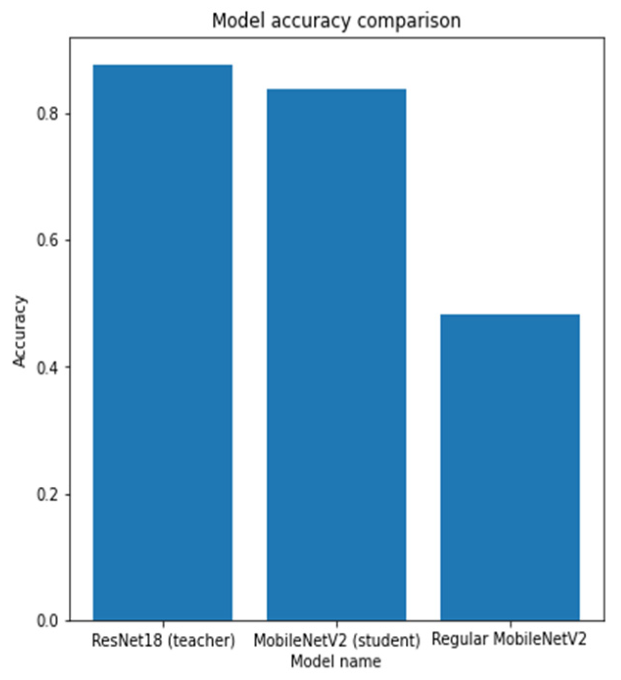
3.4.6. Model Distillation
- Base—initial ResNet18 model;
- PR—pruning method applied on the ResNet18 model;
- CL KPP 32—weight clustering, using KMeans++ for centroid initialization and 32 clusters applied on ResNet18 model;
- CL LIN 32—weight clustering, using linear centroid initialization and 32 clusters applied on the ResNet18 model;
- CL KPP 256—weight clustering, using KMeans++ for centroid initialization and 256 clusters applied on ResNet18 model;
- QAT—quantization-aware training applied on ResNet18 model;
- PCQAT PR—combined method, pruning part of the method applied on ResNet18 model;
- PCQAT CL—combined method, weight clustering part of the method applied on ResNet18 model;
- PCQAT QAT—combined method, quantization-aware training part of the method applied on ResNet18 model;
- Distillation—knowledge distillation of MobileNetV2 model from ResNet18 model.
4. Final Comparisons
- The model execution time;
- The model accuracy;
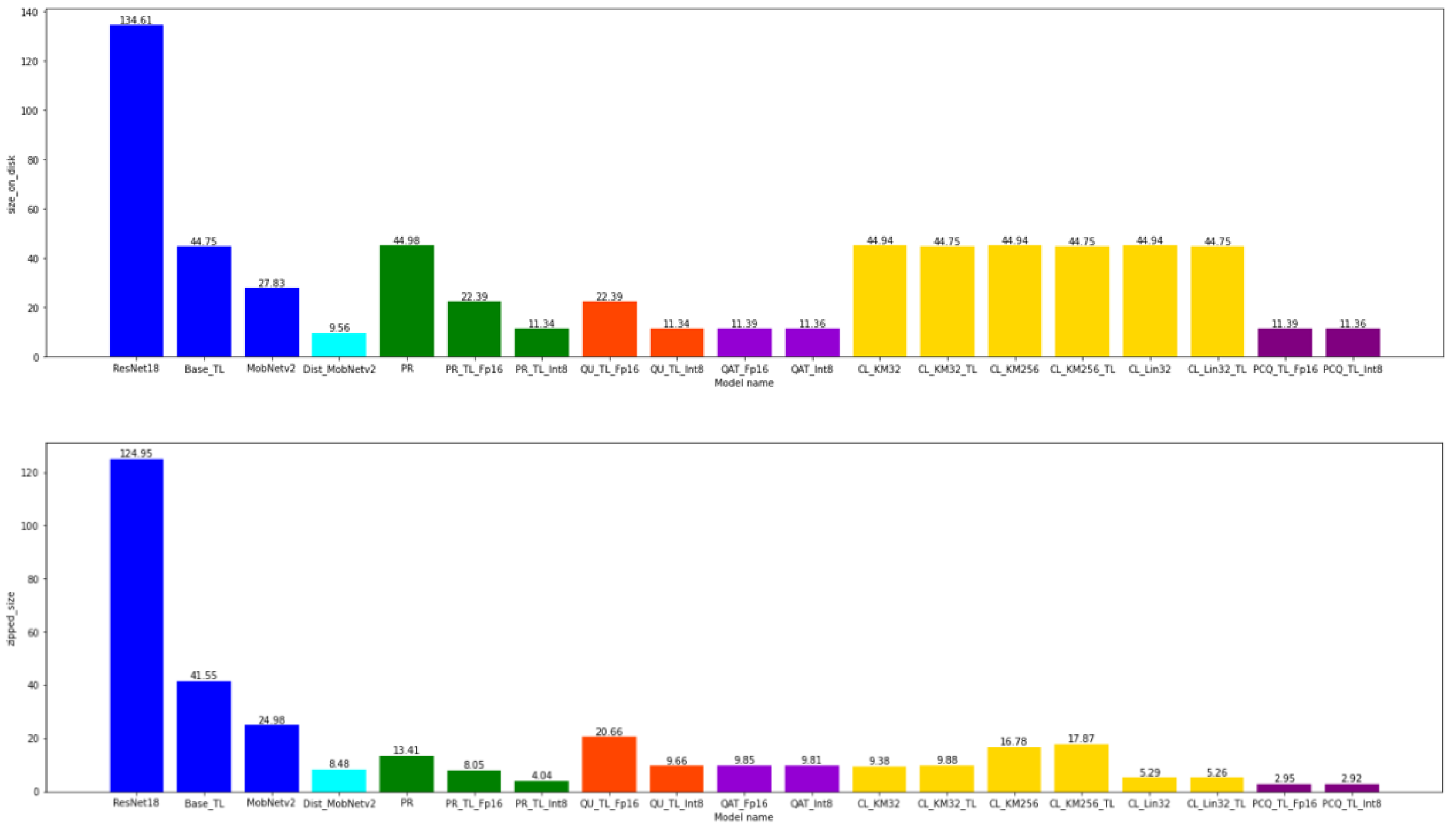
- The model size;
- The model size after the zip-function-enabled compression.
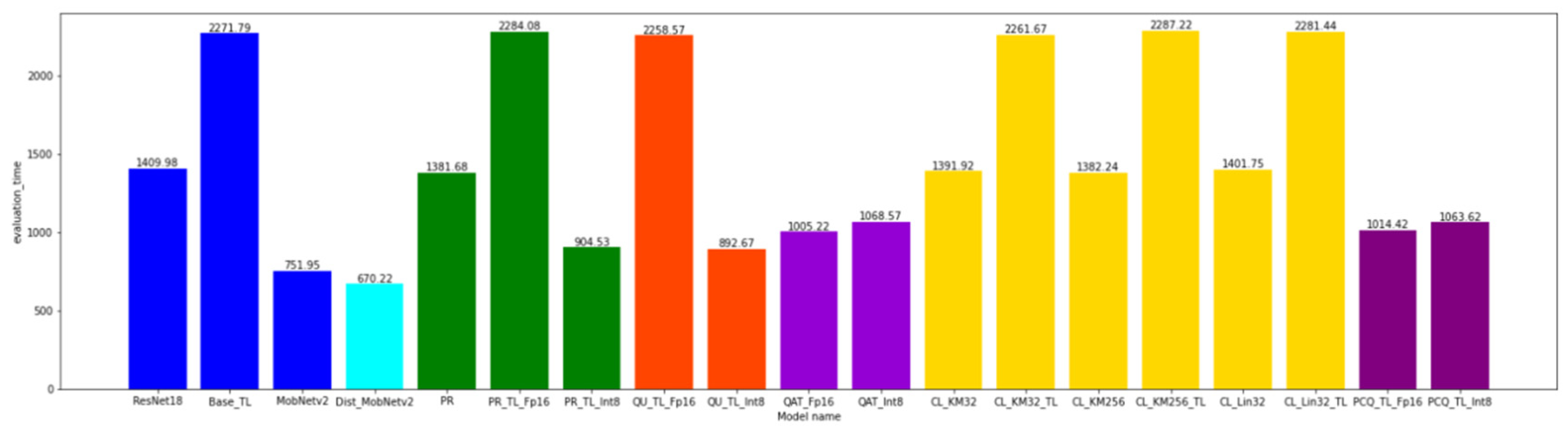
4.1. The Model Execution Time
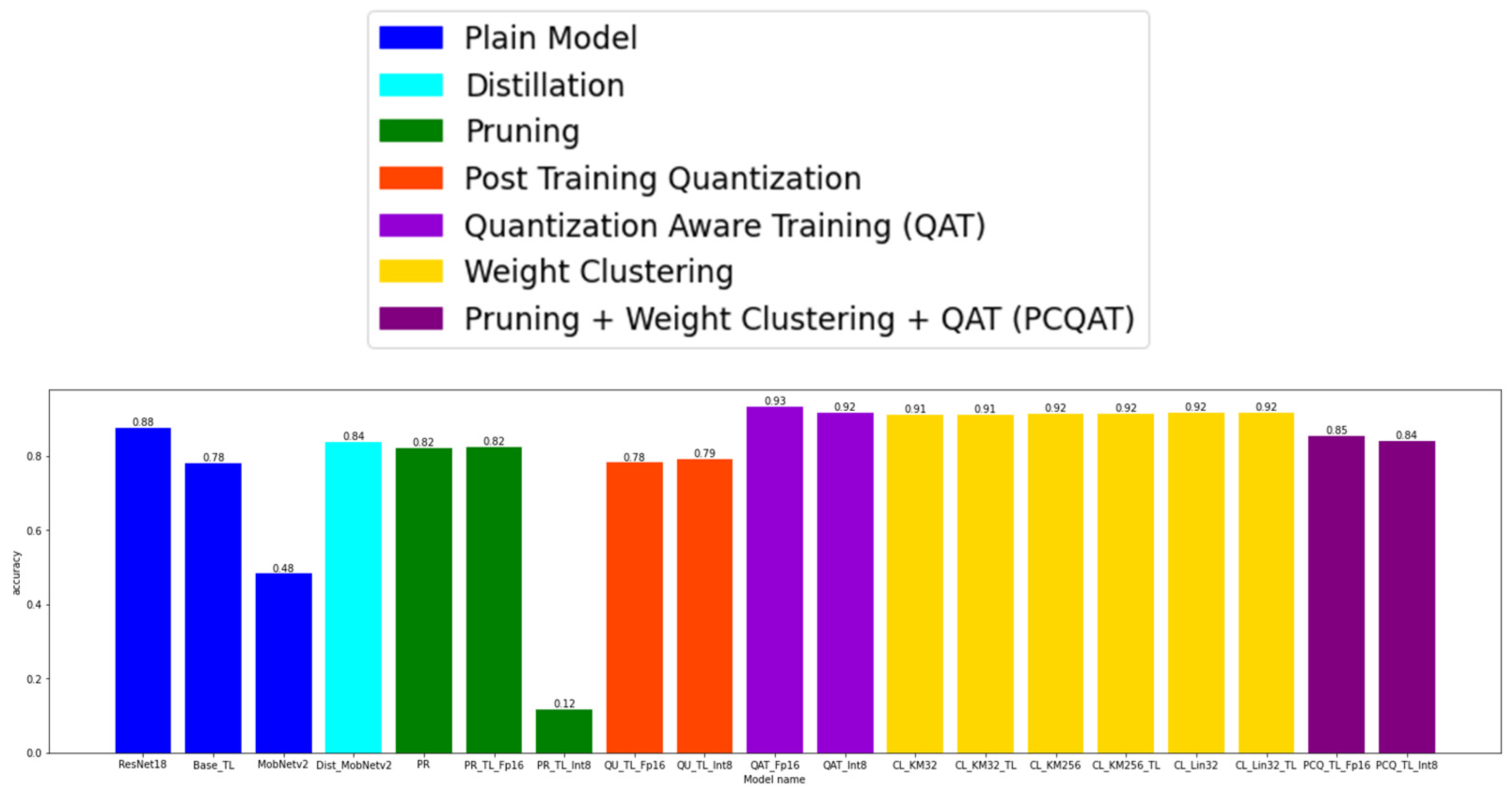
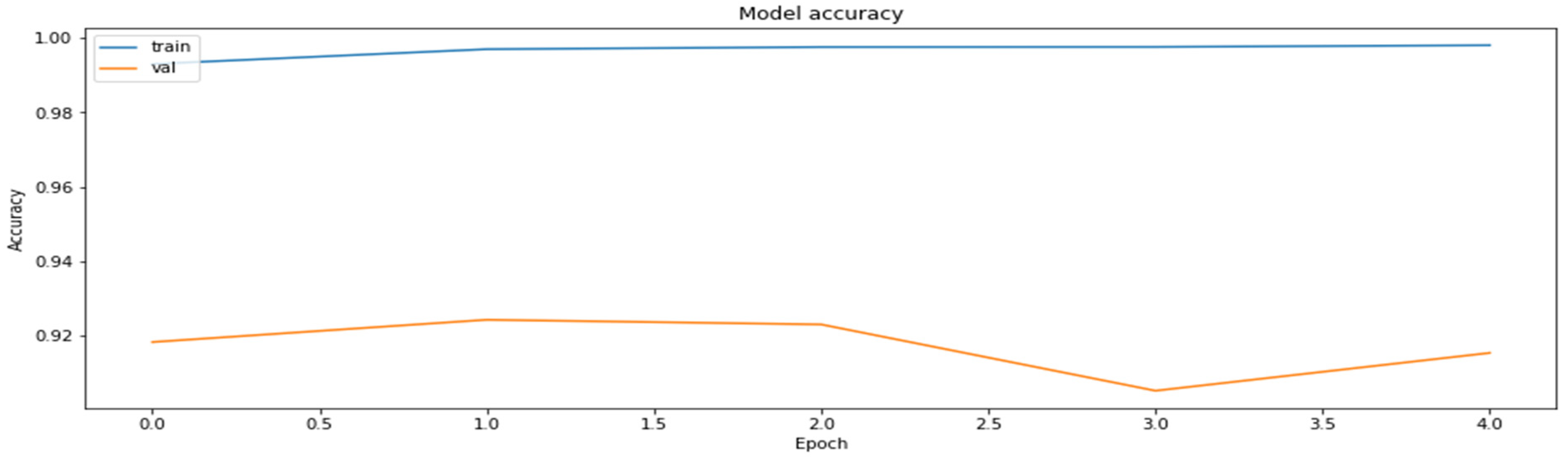
4.2. The Model Accuracy
4.3. The Model Size
4.4. The Model Size after the Zip-Function-Enabled Compression
4.5. Recommendations for the Application of Compression with Tensorflow Library
5. Conclusions
Author Contributions
Funding
Data Availability Statement
Conflicts of Interest
Appendix A


References
- Kotenko, I.; Izrailov, K.; Buinevich, M. Static Analysis of Information Systems for IoT Cyber Security: A Survey of Machine Learning Approaches. Sensors 2022, 22, 1335. [Google Scholar] [CrossRef] [PubMed]
- Shenbagalakshmi, V.; Jaya, T. Application of machine learning and IoT to enable child safety at home environment. J. Supercomput. 2022, 78, 10357–10384. [Google Scholar] [CrossRef]
- Mohammadi, F.G.; Shenavarmasouleh, F.; Arabnia, H.R. Applications of Machine Learning in Healthcare and Internet of Things (IOT): A Comprehensive Review. arXiv 2022, arXiv:2202.02868. [Google Scholar]
- Mohammed, C.M.; Askar, S. Machine learning for IoT healthcare applications: A review. Int. J. Sci. Bus. 2021, 5, 42–51. [Google Scholar]
- Hamad, Z.J.; Askar, S. Machine Learning Powered IoT for Smart Applications. Int. J. Sci. Bus. 2021, 5, 92–100. [Google Scholar]
- Atul, D.J.; Kamalraj, R.; Ramesh, G.; Sankaran, K.S.; Sharma, S.; Khasim, S. A machine learning based IoT for providing an intrusion detection system for security. Microprocess. Microsyst. 2021, 82, 103741. [Google Scholar] [CrossRef]
- Murdoch, W.J.; Singh, C.; Kumbier, K.; Abbasi-Asl, R.; Yu, B. Definitions, methods, and applications in interpretable machine learning. Proc. Natl. Acad. Sci. USA 2019, 116, 22071–22080. [Google Scholar] [CrossRef] [Green Version]
- Chen, R.-C.; Dewi, C.; Huang, S.-W.; Caraka, R.E. Selecting critical features for data classification based on machine learning methods. J. Big Data 2020, 7, 1–26. [Google Scholar] [CrossRef]
- Abdulhammed, R.; Musafer, H.; Alessa, A.; Faezipour, M.; Abuzneid, A. Features dimensionality reduction ap-proaches for machine learning based network intrusion detection. Electronics 2019, 8, 322. [Google Scholar] [CrossRef] [Green Version]
- Murdoch, W.J.; Singh, C.; Kumbier, K.; Abbasi-Asl, R.; Yu, B. Interpretable machine learning: Definitions, methods, and applications. arXiv 2019, arXiv:1901.04592. [Google Scholar] [CrossRef] [Green Version]
- Helm, J.M.; Swiergosz, A.M.; Haeberle, H.S.; Karnuta, J.M.; Schaffer, J.L.; Krebs, V.E.; Spitzer, A.I.; Ramkumar, P.N. Machine Learning and Artificial Intelligence: Definitions, Applications, and Future Directions. Curr. Rev. Musculoskelet. Med. 2020, 13, 69–76. [Google Scholar] [CrossRef] [PubMed]
- Canziani, A.; Paszke, A.; Culurciello, E. An analysis of deep neural network models for practical applications. arXiv 2016, arXiv:1605.07678. [Google Scholar]
- Sze, V.; Chen, Y.-H.; Yang, T.-J.; Emer, J.S. Efficient Processing of Deep Neural Networks: A Tutorial and Survey. Proc. IEEE 2017, 105, 2295–2329. [Google Scholar] [CrossRef] [Green Version]
- Anbarasan, M.; Muthu, B.; Sivaparthipan, C.; Sundarasekar, R.; Kadry, S.; Krishnamoorthy, S.; Dasel, A.A. Detection of flood disaster system based on IoT, big data and convolutional deep neural network. Comput. Commun. 2020, 150, 150–157. [Google Scholar] [CrossRef]
- Han, S.; Mao, H.; Dally, W.J. Deep compression: Compressing deep neural networks with pruning, trained quantization and Huffman coding. arXiv 2015, arXiv:1510.00149. [Google Scholar]
- Lakhan, A.; Mastoi, Q.-U.; Elhoseny, M.; Memon, M.S.; Mohammed, M.A. Deep neural network-based application partitioning and scheduling for hospitals and medical enterprises using IoT assisted mobile fog cloud. Enterp. Inf. Syst. 2021, 15, 1–23. [Google Scholar] [CrossRef]
- Sattler, F.; Wiegand, T.; Samek, W. Trends and advancements in deep neural network communication. arXiv 2020, arXiv:2003.03320. [Google Scholar]
- Verhelst, M.; Moons, B. Embedded Deep Neural Network Processing: Algorithmic and Processor Techniques Bring Deep Learning to IoT and Edge Devices. IEEE Solid-State Circuits Mag. 2017, 9, 55–65. [Google Scholar] [CrossRef]
- Mehra, M.; Saxena, S.; Sankaranarayanan, S.; Tom, R.J.; Veeramanikandan, M. IoT based hydroponics system using Deep Neural Networks. Comput. Electron. Agric. 2018, 155, 473–486. [Google Scholar] [CrossRef]
- Thakkar, A.; Chaudhari, K. A comprehensive survey on deep neural networks for stock market: The need, challenges, and future directions. Expert Syst. Appl. 2021, 177, 114800. [Google Scholar] [CrossRef]
- Brajević, I.; Brzaković, M.; Jocić, G. Solving integer programming problems by using population-based beetle antennae search algorithm. J. Process Manag. New Technol. 2021, 9, 89–99. [Google Scholar] [CrossRef]
- Abdou, M.A. Literature review: Efficient deep neural networks techniques for medical image analysis. Neural Comput. Appl. 2022, 34, 5791–5812. [Google Scholar] [CrossRef]
- Fang, X.; Liu, H.; Xie, G.; Zhang, Y.; Liu, D. Deep Neural Network Compression Method Based on Product Quantization. In Proceedings of the 39th Chinese Control Conference (CCC), Shenyang, China, 27–30 July 2020. [Google Scholar] [CrossRef]
- Anwar, S.; Hwang, K.; Sung, W. Structured Pruning of Deep Convolutional Neural Networks. ACM J. Emerg. Technol. Comput. Syst. 2017, 13, 1–18. [Google Scholar] [CrossRef] [Green Version]
- Li, H.; Kadav, A.; Durdanovic, I.; Samet, H.; Graf, H.P. Pruning Filters for Efficient ConvNets. arXiv 2016, arXiv:1608.08710. [Google Scholar]
- Chen, W.; Wilson, J.T.; Tyree, S.; Weinberger, K.Q.; Chen, Y. Compressing Neural Networks with the Hashing Trick. In Proceedings of the 32nd International Conference on Machine Learning, Lille, France, 6–11 July 2015. [Google Scholar]
- Hinton, G.; Vinyals, O.; Dean, J. Distilling the Knowledge in a Neural Network. arXiv 2015, arXiv:1503.02531. [Google Scholar]
- Bucila, C.; Caruana, R.; Niculescu-Mizil, A. Model compression. In Proceedings of the 12th ACM SIGKDD International Conference on Knowledge Discovery and Data Mining, KDD ’06, New York, NY, USA, 20–23 August 2006; ACM: New York, NY, USA; pp. 535–541. [Google Scholar]
- Gou, J.; Yu, B.; Maybank, S.J.; Tao, D. Knowledge Distillation: A Survey. Int. J. Comput. Vis. 2021, 129, 1789–1819. [Google Scholar] [CrossRef]
- Cai, H.; Gan, C.; Wang, T.; Zhang, Z.; Han, S. Once-for-All: Train One Network and Specialize It for Efficient Deployment. arXiv 2019, arXiv:1908.09791. [Google Scholar]
- Luo, J.-H.; Wu, J.; Lin, W. ThiNet: A Filter Level Pruning Method for Deep Neural Network Compression. In Proceedings of the IEEE International Conference on Computer Vision (ICCV), Venice, Italy, 22–29 October 2017; Institute of Electrical and Electronics Engineers (IEEE): Piscataway, NJ, USA, 2017; pp. 5068–5076. [Google Scholar]
- Duan, X.; Guo, D.; Qin, C. Image Information Hiding Method Based on Image Compression and Deep Neural Network. Comput. Model. Eng. Sci. 2020, 124, 721–745. [Google Scholar] [CrossRef]
- Chen, R.; Chen, Y.; Su, J. Deep convolutional neural networks compression method based on linear representation of kernels. In Proceedings of the Eleventh International Conference on Machine Vision (ICMV 2018), Munich, Germany, 30 November 2018; 11041, p. 110412N. [Google Scholar] [CrossRef]
- Sun, S.; Chen, W.; Bian, J.; Liu, X.; Liu, T. Ensemble-Compression: A New Method for Parallel Training of Deep Neural Networks. Machine Learning and Knowledge Discovery in Databases. In Lecture Notes in Artificial Intelligence; ECML PKDD 2017, PT I; Book Series; Volume 10534, pp. 187–202. [CrossRef] [Green Version]
- Salehinejad, H.; Valaee, S. Ising-dropout: A Regularization Method for Training and Compression of Deep Neural Networks. In Proceedings of the ICASSP IEEE International Conference on Acoustics, Speech and Signal Processing (ICASSP), Brighton, UK, 12–17 May 2019; pp. 3602–3606. [Google Scholar] [CrossRef] [Green Version]
- Yamagiwa, S.; Yang, W.; Wada, K. Adaptive Lossless Image Data Compression Method Inferring Data Entropy by Applying Deep Neural Network. Electronics 2022, 11, 504. [Google Scholar] [CrossRef]
- Zeng, L.; Chen, S.; Zeng, S. An Efficient End-to-End Channel Level Pruning Method for Deep Neural Networks Compression. In Proceedings of the IEEE 10th International Conference on Software Engineering and Service Science (ICSESS), Beijing, China, 18–20 October 2019; pp. 43–46. [Google Scholar] [CrossRef]
- Ademola, O.A.; Leier, M.; Petlenkov, E. Evaluation of Deep Neural Network Compression Methods for Edge Devices Using Weighted Score-Based Ranking Scheme. Sensors 2021, 21, 7529. [Google Scholar] [CrossRef]
- Kather, J.N.; Halama, N.; Marx, A. Zenodo. Available online: https://zenodo.org/record/1214456#.YZkx57so9hF (accessed on 12 December 2021).
- Macenko, M.; Niethammer, M.; Marron, J.S.; Borland, D.; Woosley, J.T.; Guan, X.; Schmitt, C.; Thomas, N.E. A Method For Normalizing Histology Slides For Quantitative Analysis. In Proceedings of the IEEE International Symposium on Biomedical Imaging, Boston, MA, USA, 28 June–1 July 2009. [Google Scholar]
- Yakubovskiy, P. Classification Models Zoo—Keras (and TensorFlow Keras). Available online: https://pypi.org/project/image-classifiers (accessed on 12 December 2021).
- TensorFlow Model Optimization Toolkit. Available online: https://www.tensorflow.org/model_optimization/guide (accessed on 3 May 2022).
- Zhou, Y.; Yen, G.G.; Yi, Z. A Knee-Guided Evolutionary Algorithm for Compressing Deep Neural Networks. IEEE Trans. Cybern. 2019, 51, 1626–1638. [Google Scholar] [CrossRef] [PubMed]
- dos Santos, M.; Costa, I.P.d.A.; Gomes, C.F.S. Multicriteria decision-making in the selection of warships: A new approach to the ahp method. Int. J. Anal. Hierarchy Process 2021, 13, 147–169. [Google Scholar] [CrossRef]


| Base | FP16 | INT16 | Full INT8 | |
|---|---|---|---|---|
| Accuracy | 78.14 | 78.24 | 78.14 | 79.24 |
| Base | PR | CL KPP 32 | CL LIN 32 | CL KPP 256 |
| 1107 | 1260.5 | 1089.6 | 1109.2 | 1132.8 |
| QAT | PCQAT PR | PCQAT CL | PCQAT QAT | Distillation |
| 1164.8 | 1113.25 | 1137.67 | 1214.43 | 1192.9 |
Publisher’s Note: MDPI stays neutral with regard to jurisdictional claims in published maps and institutional affiliations. |
© 2022 by the authors. Licensee MDPI, Basel, Switzerland. This article is an open access article distributed under the terms and conditions of the Creative Commons Attribution (CC BY) license (https://creativecommons.org/licenses/by/4.0/).
Share and Cite
Predić, B.; Vukić, U.; Saračević, M.; Karabašević, D.; Stanujkić, D. The Possibility of Combining and Implementing Deep Neural Network Compression Methods. Axioms 2022, 11, 229. https://doi.org/10.3390/axioms11050229
Predić B, Vukić U, Saračević M, Karabašević D, Stanujkić D. The Possibility of Combining and Implementing Deep Neural Network Compression Methods. Axioms. 2022; 11(5):229. https://doi.org/10.3390/axioms11050229
Chicago/Turabian StylePredić, Bratislav, Uroš Vukić, Muzafer Saračević, Darjan Karabašević, and Dragiša Stanujkić. 2022. "The Possibility of Combining and Implementing Deep Neural Network Compression Methods" Axioms 11, no. 5: 229. https://doi.org/10.3390/axioms11050229
APA StylePredić, B., Vukić, U., Saračević, M., Karabašević, D., & Stanujkić, D. (2022). The Possibility of Combining and Implementing Deep Neural Network Compression Methods. Axioms, 11(5), 229. https://doi.org/10.3390/axioms11050229