Abstract
In the paper, the possibility of combining deep neural network (DNN) model compression methods to achieve better compression results was considered. To compare the advantages and disadvantages of each method, all methods were applied to the ResNet18 model for pretraining to the NCT-CRC-HE-100K dataset while using CRC-VAL-HE-7K as the validation dataset. In the proposed method, quantization, pruning, weight clustering, QAT (quantization-aware training), preserve cluster QAT (hereinafter PCQAT), and distillation were performed for the compression of ResNet18. The final evaluation of the obtained models was carried out on a Raspberry Pi 4 device using the validation dataset. The greatest model compression result on the disk was achieved by applying the PCQAT method, whose application led to a reduction in size of the initial model by as much as 45 times, whereas the greatest model acceleration result was achieved via distillation on the MobileNetV2 model. All methods led to the compression of the initial size of the model, with a slight loss in the model accuracy or an increase in the model accuracy in the case of QAT and weight clustering. INT8 quantization and knowledge distillation also led to a significant decrease in the model execution time.
Keywords:
deep learning; convolutional neural networks; deep neural network model; combining methods; implementation MSC:
68T05
1. Introduction
In the past few years, we have been witnessing the ever-increasing application of machine learning and deep learning to create applications on mobile (smart) phones and Internet of Things (IoT) devices [1,2,3,4,5,6]. The main feature of the methods based on machine learning is extracting the characteristics (i.e., features) from within a large number of data without human involvement [7,8,9,10,11]. Additionally, these methods generate better results than methods requiring active human participation to extract said features. Due to this fact, the solutions based on deep neural networks (DNN) have become dominant when speaking about solving numerous problems, even in the different fields of the IoT industry, including smart houses, agriculture, movement regime recognition, and so on [12,13,14]. The elements of DNN models can be divided into convolutional neural networks or layers (CNN), fully connected (FC) networks or layers, and recurrent networks or layers (RNN). A DNN model may be characterized by all of these components at once or a combination of the same components. The CNN components extract spatial characteristics whereas the RNN components extract temporal characteristics from within a dataset. Despite their great advantages, DNN models require greater resources than the other methods do, such as greater consumption of energy, greater calculation demands, and greater space requirements for storing trained models. These requirements for additional resources reduce the usability of such models when designing web, mobile, and IoT applications. To reduce these shortcomings of DNN models, a large number of compression methods have been developed. Some of the advantages of the application of compression to DNN models are as follows:
- Storing capacities: DNN models use a large number of parameters to achieve a high level of accuracy. Storing all of these parameters requires a large amount of memory. For these reasons, DNN model compression leads to reductions in size and enables their application on resource-constrained devices (RC devices).
- The complexity of calculation: While being executed, DNN models require a great number of floating-point operations per second (FLOPs). RC devices cannot achieve the number of operations required for the application of contemporary models. For that very reason, it is possible to apply compression techniques that reduce the number of calculations while using the model.
- Execution in real-time: Contemporary DNN models require a lot of time for training and execution as well, which reduces their usability for solving the problems that require data processing in real-time. Compressing a model enables us to not only reduce the calculation but also the model calculation time, meaning it is possible to apply the model when processing data in real-time.
- Privacy: If it is not possible to apply a model on an RC device, data have to be transferred via a network to a server capable of running the original model. During this data transfer process to such a server, the possibility of data protection issues and abuse increases. The application of DNN models directly on RC devices eliminates the possibility of such attacks.
- Energy consumption: RC device consumption is primarily determined by the access to the memory. For devices constructed using the 45 nm CMOS technology, a 32-bit collector consumes about 0.9 pJ of energy. That very same technology consumes 5 pJ of energy to access 32-bit data in SRAM and 640 pJ to access 32-bit data in DRAM. Contemporary DNN models cannot be fully stored in a device’s cache memory; for this reason, their execution requires multiple access to DRAM, and simultaneously also a greater consumption of electrical energy. The compression of a DNN model leads to a decrease in energy consumption during its application and prolongs the lifecycle of battery-charged IoT devices [15].
The demand for the use of DNN models on mobile and IoT devices is enormous and is increasing day after day [16,17,18,19,20,21,22]. It is sometimes impossible to apply ordinary rather than compressed models on RC devices such as these. For this reason, this paper will present a review of the basic DNN model compression methods, also enabling their use on such devices.
The aim of the study was to explore the performance, benefits, and drawbacks of DNN compression methods and the possibility of combining multiple compression methods in order to achieve better compression results. As a base model, the ResNet18 model was pretrained on the NCT-CRC-HE-100K dataset with CRC-VAL-HE-7K serving as the validation dataset. The NCT-CRC-HE dataset was chosen to obtain hands-on experience of compression methods for a real-world problem. The selected dataset contains images of sufficiently small resolution to allow processing by RC devices. The TensorFlow Model Optimization Toolkit library was used to implement various methods for quantization, pruning, weight clustering, and a combination of these methods. The TensorFlow Lite package was utilized for the final quantization stage of the models. For knowledge distillation, the Keras framework was used to create a custom class. MobileNetV2, which has three times as few parameters as the original ResNet18 model, was employed for knowledge distillation. Accordingly, the paper is structured as follows: Introductory considerations are presented in Section 1. In Section 2, related work is presented. Section 3 presents the experimental testing and results, whereas the final comparisons are presented in Section 4. Finally, at the end of the manuscript, conclusions are given.
2. Related Works
In [15], authors used a three-stage pipeline consisting of pruning, trained quantization, and Huffman coding for compressing DNN models that can afterwards be deployed on embedded systems. In the first stage, pruning is applied on a network, which leaves only important connections. After that, remaining weights are quantized in order to enforce weight sharing. Finally, in the last stage of the pipeline, quantized weights are Huffman-coded. By using the proposed method, authors managed to reduce required storage for AlexNet by 35 times (from 240 MB to 6.9 MB) and 49 times (from 552 MB to 11.3 MB) for the VGG-16 network. In both cases, there was no loss in accuracy after the compression. Similarly, authors of paper [23] used a combination of product quantization and pruning to compress deep neural networks with a large-size model and a great amount of calculation. Authors used pruning to reduce redundant parameters in the deep neural networks, and then refined the tuning network for fine-tuning. The next phase in their proposed method is product quantization to quantize the parameters of the neural network to 8 bits, which reduces the storage overhead so that the deep neural network can be deployed in embedded devices.
In [24], authors applied structured pruning for compressing a convolutional neural network (CNN) in order to avoid irregular sparsity within the network. Authors introduced structured sparsity at various scales of CNN, which exhibit channel, kernel, and intrakernel stride sparsity. This structured sparsity provides computational resource savings that can be advantageous for embedded devices, parallel computing environments, and hardware-based systems. Similarly, authors of paper [25] applied pruning by removing CNN filters that have a small effect on the output accuracy. By removing whole filters in the network along with their connecting feature maps, the computation costs are reduced significantly. Even simple filter pruning techniques can significantly reduce computational costs for VGG-16 (up to 34%) and ResNet-110 (up to 38%) on the CIFAR10 dataset without a significant drop in model accuracy.
Paper [26] proposed novel network architecture, HashedNets, for exploiting inherent redundancy in neural networks to achieve drastic reductions in model size. HashedNets uses a low-cost hash function to randomly group connection weights into hash buckets. All connections grouped into the same bucket share a single parameter value. This approach does not introduce additional memory overhead, and authors demonstrated that this architecture reduces the storage requirements of neural networks trained on several benchmark datasets while preserving generalization performance.
In [27] authors improved the method for transferring the knowledge from the ensemble model into a single model previously proposed by Caruna and his collaborators [28]. In this method, a smaller model (also known as a student model) learns to mimic the outputs of one or many much bigger models (also known as a teacher model). By softening the outputs of the Softmax layer of teacher models, the student is able to learn much more about the relation between the output classes compared to when student is trying to mimic the outputs of the teacher model. To soften the outputs of the teacher model, the authors introduced a new parameter, T (also known as temperature), which controls the softening of the teacher model output. Because of this temperature parameter, the whole process is named knowledge distillation. In paper [29], a comprehensive survey was given on knowledge distillation from the perspective of knowledge categories, training schemes, teacher–student architecture, distillation algorithms, performance comparison, and applications. In our work, we tried to use knowledge distillation as a compression method to transfer knowledge to a three-times-smaller model by preserving as much accuracy as possible. We also compared the performance of a regularly trained student model to that of a distilled student model.
In [30], authors proposed training a once-for-all (OFA) network that supports diverse architectural settings by decoupling training from a neural architecture search (NAS). This approach can quickly achieve a specialized sub-network by selecting from the OFA network without additional training. Additionally, a novel progressive shrinking algorithm was proposed, which is a generalized version of the pruning method that reduces the model size across many more dimensions than pruning.
Authors in [31] proposed an efficient and unified framework, named ThiNet, to simultaneously accelerate and compress CNN models in both training and inference stages. Authors focused on the filter level pruning, i.e., the whole filter is discarded if it is less important. Their proposed method does not change the original network structure; thus it can be perfectly supported by any off-the-shelf deep learning libraries. Paper [32] proposed a steganography framework that combines image compression. Their experimental results show that the steganographic framework guarantees the quality of steganography while its relative steganographic capacity reaches 1. Besides, Peak Signal-to-Noise Ratio (PSNR) and Structural Similarity Index (SSIM) values can reach 42 dB and 0.94, respectively.
In [33], authors present a deep convolutional neural network compression method based on the linear representation of kernels. This model was retrained with fixed template kernels, and only two related parameters needed to be fine-tuned for each kernel. Experiments show that convolutional kernels of a large CNN model can be represented using only a small number of templates. This proposed method can be performed with other compression approaches to obtain a higher compression rate.
Authors of paper [34] carried out model compression after each ensemble, specialized by a distillation-based method in this paper, to reduce the size of the global model to that of the local ones. Their experimental results demonstrate the prominent advantage of Ensemble-Compressed DNNs (EC-DNN) over Model Average DNNs (MA-DNN) in terms of both accuracy and speedup.
In [35], authors proposed an adaptive technique to wisely drop the visible and hidden units in a deep neural network using the Ising energy of the network. The preliminary results show that the proposed approach can keep the classification performance competitive at the level of the original network while eliminating the optimization of unnecessary network parameters in each training cycle. The dropout state of units can also be applied to the trained (inference) model. This technique could compress the number of parameters up to 41.18% and 55.86% for the classification task on the MNIST and Fashion-MNIST datasets, respectively.
Paper [36] especially focused on lossless compression for image data, focusing on the image blocks. Through experimental evaluation, this paper showed reasonable compression performance when the proposed method was applied rather than when a randomly selected compression program was applied to the entire dataset.
In [37], authors introduced additional auxiliary classifiers to enhance the discriminative power of shallow and intermediate layers. Secondly, the authors imposed L1-regularization on the scaling factors and shifting factors in the batch normalization (BN) layer and adopted the fast and iterative shrinkage-thresholding algorithm (FISTA) to effectively prune the redundant channels. Finally, by forcing selected factors to zero, authors could prune the corresponding unimportant channels safely, thus obtaining a compact model. They empirically revealed the prominent performance of our approach with several state-of-the-art DNN architectures, including VGGNet and MobileNet, on different datasets.
Authors in [38] showed an evaluation of deep neural network compression methods for edge devices using a weighted score-based ranking scheme. The authors demonstrated the effectiveness of their method by applying it to the baseline, compressed, and micro-CNN models trained on our dataset. The result shows that quantization is the most efficient compression method for the application, having the highest rank, with an average weighted score of 9.00, followed by binarization, having an average weighted score of 8.07. Their proposed method is extendable and can be used as a framework for the selection of suitable model compression methods for edge devices in different applications.
3. Experimental Testing and Results
At the very beginning of the work, we considered the use of a well-known dataset, such as the ImageNet dataset, first of all, due to its popularity and also because there are public pretrained models on this dataset that were subjected to consideration. By doing so, the need for model initial training is reduced, and only compression techniques can be paid attention to. That idea was, however, rejected later, namely for the following reasons:
- The ImageNet is far too large a dataset to be processed by computational resources provided for this research. The Kaggle platform provides each user of the website a total of 30 free-of-charge hours to train a model on NVIDIA TESLA P100 GPU every week. Simultaneously, one training session (committing one Kaggle kernel) must not run for more than twelve hours. Due to these limitations, the training of a model on the ImageNet dataset is almost impossible.
- In practice, problems with far fewer classes appear more frequently, where a quite specific issue should be solved.
- Using a subset of the ImageNet dataset would require additional work for selecting appropriate subset classes that are easy to train initial models on but still challenging enough to prevent it from differentiating the classes based on some simple feature, such as the most widespread image color.
- The initial (base) model trained on the selected dataset needs to have high enough accuracy so that all degradation of accuracy after model compression can be addressed to the applied compression method.
Keeping in mind the abovementioned reasons, the “100,000 histological images of human colorectal cancer and healthy tissue” [39] was selected as a dataset to be used for the method compression for the following reasons:
- The dataset is of a far smaller size, which on its part results in shorter model training.
- The images are preprocessed using Macenko’s color normalization method [40], so there is no need for additional processing.
- Simple models (ResNet18 and ResNet50) generate good results (about 90% accuracy on the validation set) after having been trained on this dataset without additional data processing, so more attention can be paid to the compression techniques themselves.
Generally speaking, the selected dataset represents a problem that can be solved by utilization of an RC device. The data were well-prepared for training DNN models and gave us a broad understanding of what we can expect from compression methods when the data are well-prepared.
3.1. Dataset and Subsets
The dataset consists of three subsets, namely NCT-CRC-HE-100K, CRC-VAL-HE-7K, and i NCT-CRC-HE-100K-NONORM.
The description of the NCT-CRC-HE-100K data subset is as follows:
- This is a set of 100,000 non-overlapping segments of the images derived from the histological images of colorectal cancer and the normal human tissue colored using hematoxylin and eosin (H&E).
- All the images are the size of 224 × 224 pixels (px) on the scale of 0.5 microns per pixel. The colors of all the images are normalized using Macenko’s method [40].
- The following tissue classes can be seen in the images: adipose (ADI), background (BACK), debris (DEB), lymphocytes (LYM), mucus (MUC), smooth muscle (MUS), normal colon mucosa (NORM), cancer-associated stroma (STR), and colorectal adenocarcinoma epithelium (TUM).
- The images were selected manually from the N = 86 H&E-colored parts of the human cancerogenic tissue using the formalin-fixed paraffin-embedded (FFPE) formalin obtained from the NCT Biobank (National Center for Tumor Diseases, Heidelberg, Germany) and the pathology archive of the UMM (University Medical Center Mannheim, Mannheim, Germany). The tissue samples contained CRC primary tumor samples, as well as tumor tissue, from the CRC metastases in the liver. The normal tissue classes were augmented with the non-tumor samples to increase variability.
The description of the CRC-VAL-HE-7K data subset is as follows:
- This is a set of 7180 segments of the images obtained from a total of 50 patients with colorectal adenocarcinoma.
- There is no overlapping in-between the patients used to generate this set and the patients used to generate the NCT-CRC-HE-100K set.
- This set can be used as a validation set for the models trained on a larger set (NCT-CRC-HE-100K). As in the first dataset, the image segments are the size of 224 × 224 px with a scale of 0.5 microns per pixel. All the samples were obtained from the NCT Tissue Bank.
The description of the NCT-CRC-HE-100K-NONORM data subset is as follows:
- This is a different version of the NCT-CRC-HE-100K dataset.
- This set contains 100,000 image segments of the nine tissue classes with a scale of 0.5 microns per pixel.
- The same was created based upon the same data as the NCT-CRC-HE-100K set but deprived of image color normalization. For that reason, the intensity of the coloring and the color itself vary from one image to the next. Although this set was generated from the same data as NCT-CRC-HE-100K, the image segments are not completely the same, since the selection of non-overlapping segments is a stochastic process.
The previously mentioned NCT-CRC-HE-100K dataset was used to train the base model and the models during compression. The CRC-VAL-HE-7K dataset was used to validate the model. Based on these two datasets, two image generators were created. During the creation of the model training data loader, the parameters for the horizontal and vertical flips and the image random rotation were defined. This serves to achieve the data augmentation that has now already been considered a standard for training convolutional networks.
3.2. Base Model
ResNet18 was chosen as the base model on which the neural network compression methods were tested and compared with each other. The reasons for having chosen this particular model are as follows:
- ResNet networks are a very popular solution to solving diverse issues;
- ResNet18 is the simplest model generating quite acceptable results on a selected dataset (about 90% accuracy), without any additional input data processing (except for the already performed color normalization). This is a very important fact enabling us to compare the performances of the methods neglecting the impact of the data quality on the results obtained by each of the methods.
Given the fact that the ResNet18 model is not present in the set of the pretrained Keras models, the image-classifiers [41] library that extends the Keras set with additional models was used for the implementation of this model. The weights obtained through these models were pretrained on the ImageNet dataset and can be loaded for each of the models.
To the base architecture of the network, the ImageNet classifier located at the very end of the network (include top = False) was excluded, and the GlobalAveragePooling layer and the Dense layer with the number of the outputs matching the number of the classes in the dataset performing the final classification using the softmax function were added instead. Training the model from scratch did not show any significant accuracy difference, so ImageNet-pretrained weights were preferred because of already existing feature selectors.
3.3. Model Comparison Metric
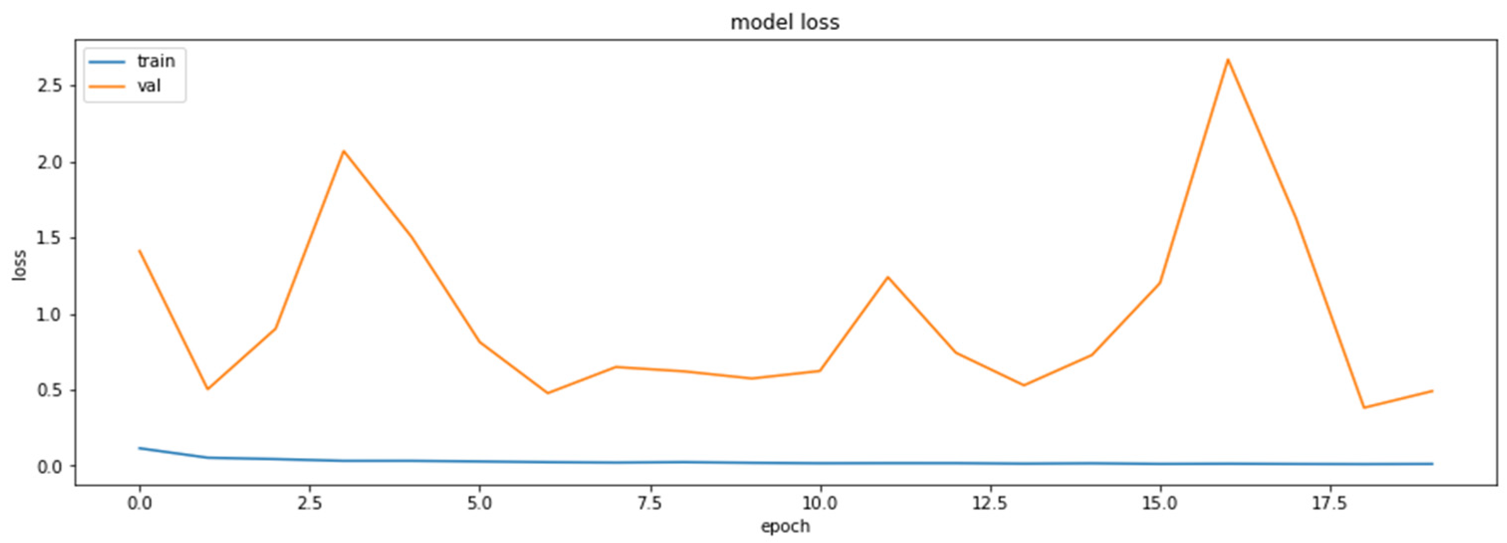
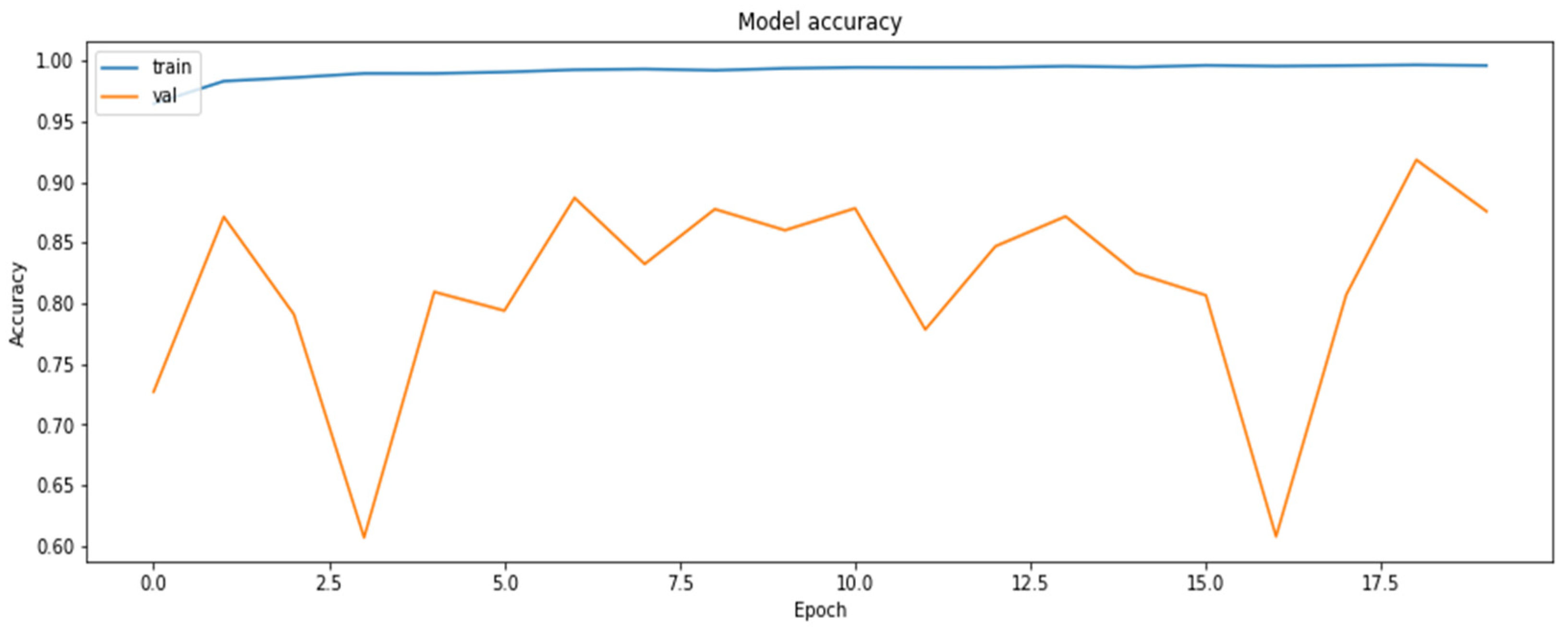
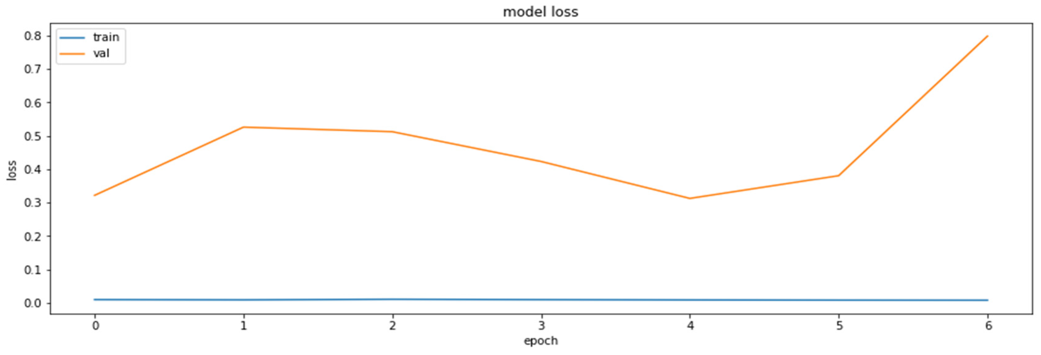
Accuracy was chosen as a metric for comparing results obtained by the models (later also for the results of the compressed models). It is also sensible to use other metrics as well, such as precision and recall, on the concrete dataset since the dataset deals with the diseased tissue classification. To compare the performances of the compressed models, however, accuracy is just a sufficient metric. The results of the training of the base model are demonstrated in Figure 1 and Figure 2.
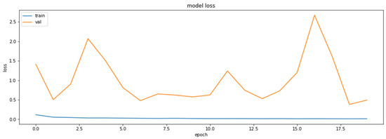
Figure 1.
The loss function values for the training and the validation datasets obtained based on RestNet18 model.
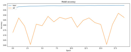
Figure 2.
The accuracy of the model for the training and the validation datasets obtained based on RestNet18 model.
As can be seen, the model can reach an up-to-90% accuracy on the validation set during the training.
3.4. Model Compression Techniques
The TensorFlow Model Optimization Toolkit (TFMOT) library [42] was used for the implementation of pruning, quantization-aware training (QAT), and weight clustering techniques. Primarily, the library is used for optimization and compression of the models and is frequently combined with the TensorFlow Lite library that enables the conversion of the existing models into the “Lite” models optimized for RC devices. Apart from the implementation of the basic compression techniques (pruning, QAT, and weight clustering), the TFMOT also enables the methods for combining these techniques:
- Cluster Preserving Quantization (CQAT)—this includes the application of the QAT technique after the application of the weight clustering technique, during whose implementation the number of the extracted clusters is retained during the model training;
- Sparsity-Preserving Quantization (PQAT)—this encompasses the application of the QAT technique after the application of the weight clustering technique, on which occasion the number of the cut-off weights is retained during the model testing;
- Sparsity-Preserving Clustering—this includes the application of the weight clustering technique after the application of the weight clustering technique, during which the number of the cut-off weights is retained during the extracting of the clusters;
- Sparsity- and Cluster-Preserving Quantization (PCQAT)—this includes the application of all three techniques (pruning, weight clustering, and QAT, in the given order), simultaneously retaining the minimum number of the cut-off weights as well as the number of the clusters that have been extracted.
3.4.1. Pruning
In the current version of the TFMOT library, there are only two implementations of the pruning_schedule, as follows:
- ConstantSparsity—the schedule which enables us to achieve the constant cutting-off value during the training;
- PolynomialDecay—the schedule that defines the value of the number of the parameters that have been cut off. During the training, the starting value of the pruning is first applied, and the value of the cut-off parameters is then increased during training all until the final value of the cut-off parameters has been achieved. This schedule mainly generates better results than the ConstantSparsity schedule since the network is being adapted during the training to use an ever-decreasing number of parameters.
The results of the application of the pruning technique with the PolynomialDecay schedule are shown in Figure 3 and Figure 4.

Figure 3.
The loss function values on the training datasets obtained by polynomial iterative pruning of the model.
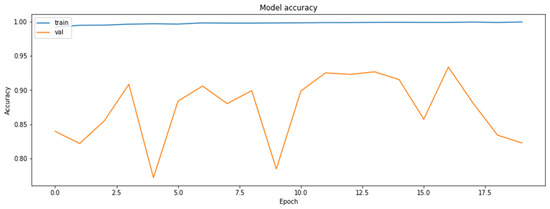
Figure 4.
The accuracy of the model on the training and the validation datasets by polynomial iterative model.
3.4.2. Post-Training Quantization
The TensorFlow Lite (TF Lite) library was used for the implementation of the quantization of the Keras model. TF Lite supports both integer and float quantization. With integer quantization, FP32 values are converted into INT values. This itself reduces the model execution time, and if a smaller number of bits are used for the presentation of INT values, then there is also a reduction in the model size. Models optimized in this way are mainly applied to small-capacity devices, such as microcontrollers, or on Edge TPU devices. One important note about the TF Lite quantization is that only INT8 quantization is supported at the runtime of the model, whereby all the other quantizations are actually converted to FP32 values at the runtime. Having this in mind, we could only expect speedup of the models quantized with INT8 quantization. The accuracies of the models obtained through the quantization of the base model with the help of the TF Lite library are accounted for below (see Table 1).

Table 1.
The accuracies of the models obtained by post-training quantization.
3.4.3. Quantization-Aware Training (QAT)
The obtained model was further compiled with the base model’s parameters and trained.
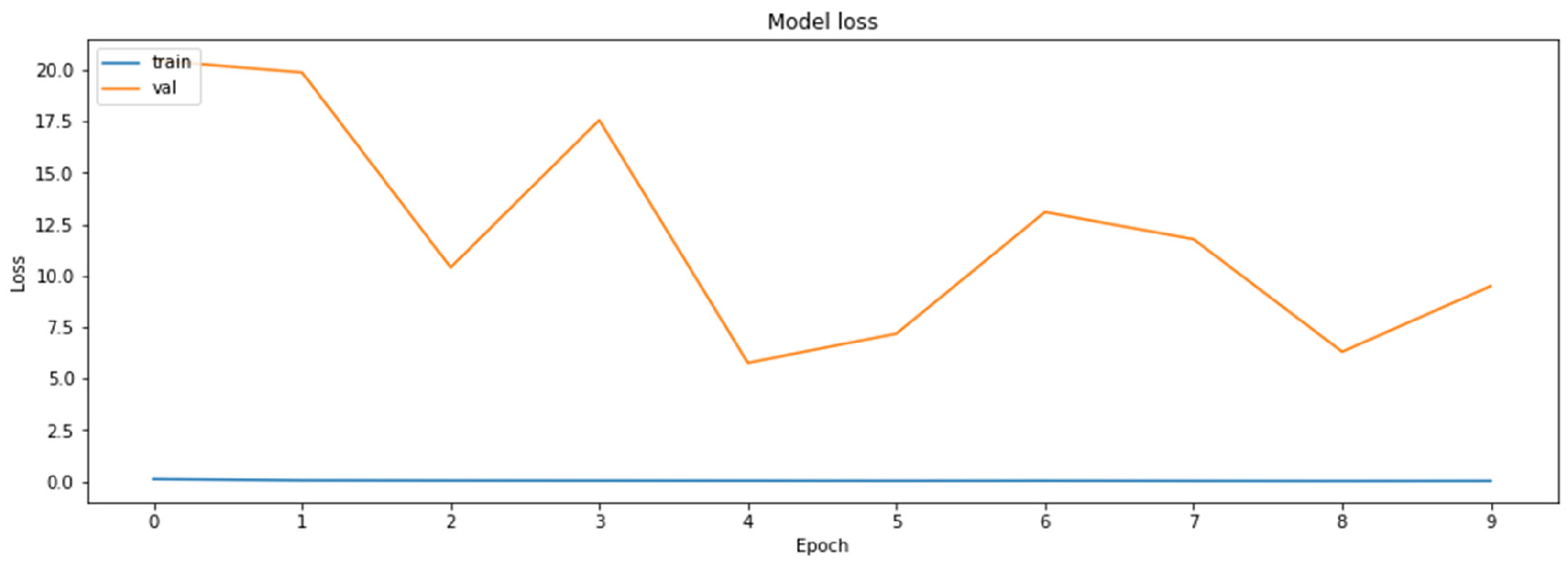
Quantization-aware training can be used to alleviate model accuracy drops caused by the quantization process by training the model to work with less accurate weights. TFMOT supports the QAT process for most of the standard layers, but in the case unsupported layers, custom layer quantization must be implemented. The training results of QAT applied on the base model can be seen in Figure 5 and Figure 6.
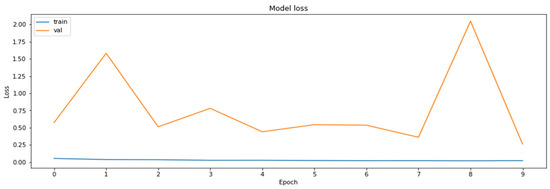
Figure 5.
The loss function values on the training and the validation datasets obtained during the training with the application of the QAT method.
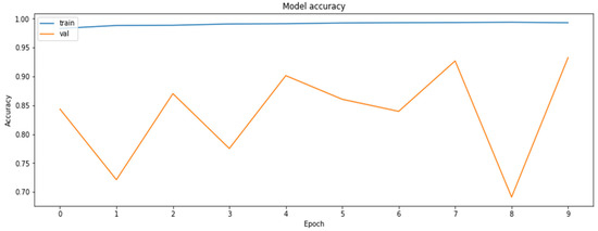
Figure 6.
The accuracy of the model on the training and the validation datasets obtained during the training with the application of the QAT method.
3.4.4. Weight Clustering
The current version of the TFMOT library supports the following algorithms for centroid initialization of clusters: LINEAR, RANDOM, DENSITY_BASED I, and KMEANS_PLUS_PLUS. Results of weight clustering training can be seen in the Appendix A (Figure A1, Figure A2, Figure A3, Figure A4, Figure A5 and Figure A6).
3.4.5. Combined Method
The combination of the pruning, weight clustering, and quantization-aware training techniques apply the pruning technique, then the weight clustering technique, retaining the percentage of cut-off weights, and ultimately the QAT technique, which retains the percentage of cut-off weights and the number of extracted clusters.
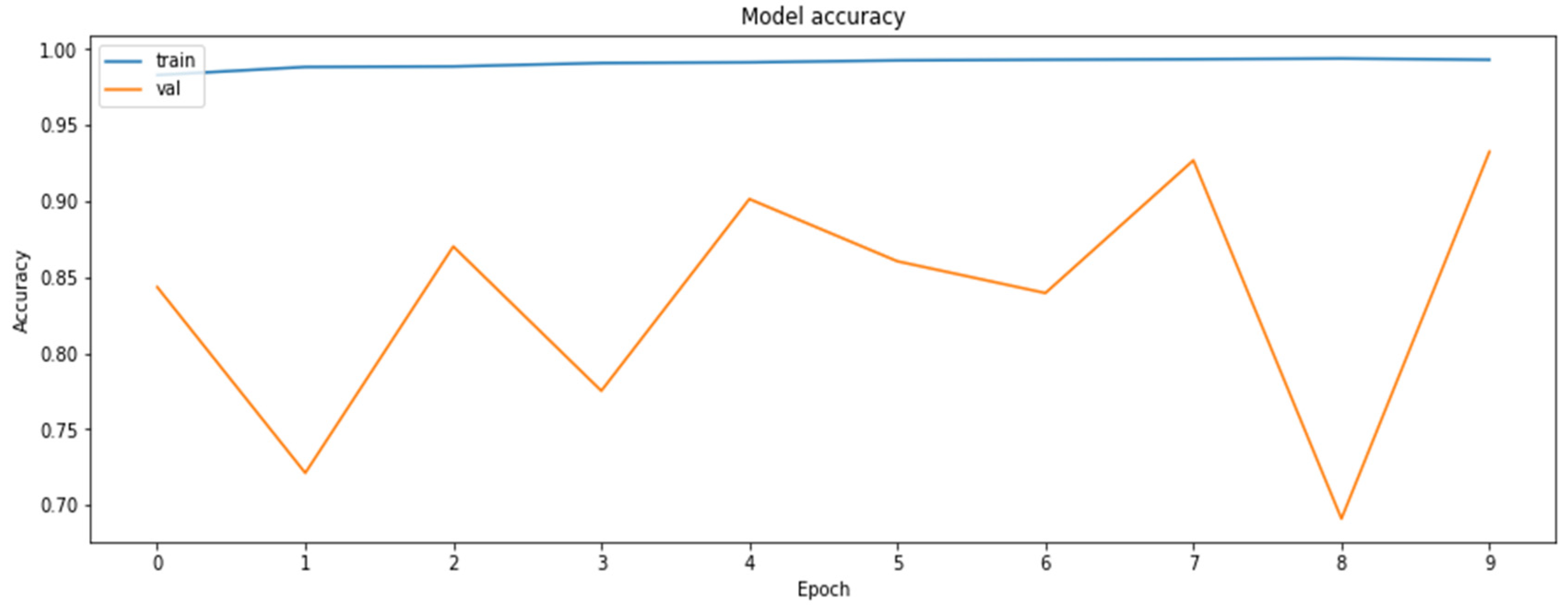
The results of applying the pruning part of the algorithm on the base model are presented in Figure 7 and Figure 8.

Figure 7.
Training and validation datasets obtained during the application of the pruning part of the PCQAT.

Figure 8.
Training and the validation datasets obtained during the application of the pruning part of the PCQAT.
After that, we applied weight clustering to the pruned model, enabling preservation of the sparsity flag, which ensured the preservation of the percentage of the cut-off weights during weight clustering. The results of the training of this part of the algorithm are shown in Figure 9 and Figure 10.

Figure 9.
Training and the validation datasets obtained during the implementation of the weight clustering of the PCQAT.

Figure 10.
Training and the validation datasets obtained during the application of the weight clustering part of the PCQAT.
Finally, QAT was applied on the weight-clustered model, and sparsity-preserving and cluster-preserving flags were set in order to maintain the compression achieved by previous methods. The results of the training of this part of the algorithm are shown in Figure 11 and Figure 12.
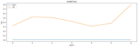
Figure 11.
The loss function values for the training and the validation datasets based on QAT part of the PCQAT method.

Figure 12.
The accuracy of the model for the training and the validation datasets based on the QAT part of the PCQAT method.
3.4.6. Model Distillation
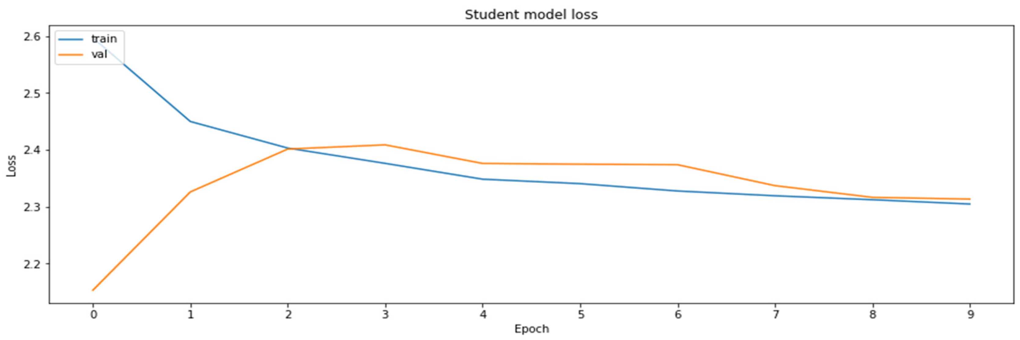
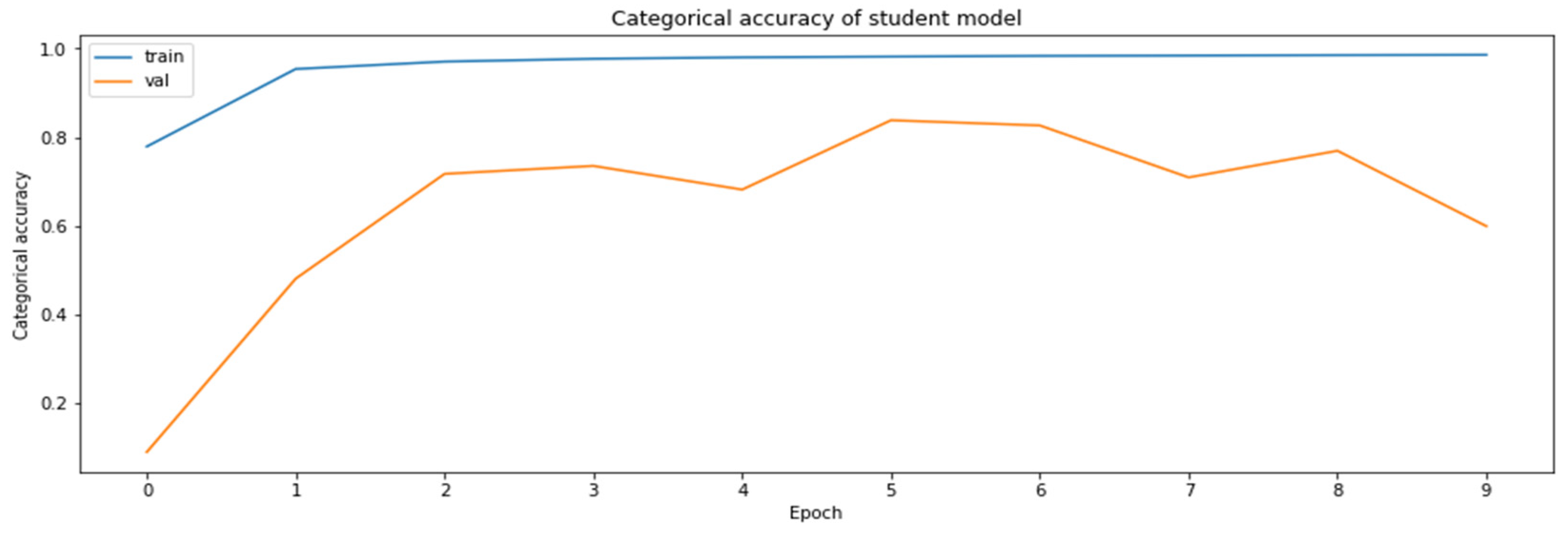
Since the primary goal was to compress the original model as much as possible while retaining as much of the original accuracy as possible, knowledge distillation was considered as a method to transfer the knowledge of the original model to a smaller model, and by doing so, it could be considered as a compression method. For this reason, the MobileNetV2 model, which is three times smaller than the initial ResNet18 model according to the number of the parameters (the ResNet18 model has about 11 million parameters, whereas the MobileNetV2 has about 3.5 million), was selected as the student model for the distillation process. For the needs of the application of distillation, the Distiller class, whose implementation can be referred to at the end of the paper, was used. The loss function used during the distillation process represents a combination of the student loss function and the distillation loss function (as proposed in the paper [27]).
loss = self.alpha ∗ student_loss + (1 − self.alpha) ∗ distillation_loss
The alpha parameter that determined the share of the student and distillation loss values against the final loss was ALPHA = 0.1, whereas the value of the temperature at which distillation was performed was TEMPERATURE = 10. The results obtained by distillation are shown in Figure 13 and Figure 14.

Figure 13.
Training and the validation datasets obtained during the model distillation process.
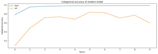
Figure 14.
The accuracy of the model for the validation datasets obtained during the model distillation process.
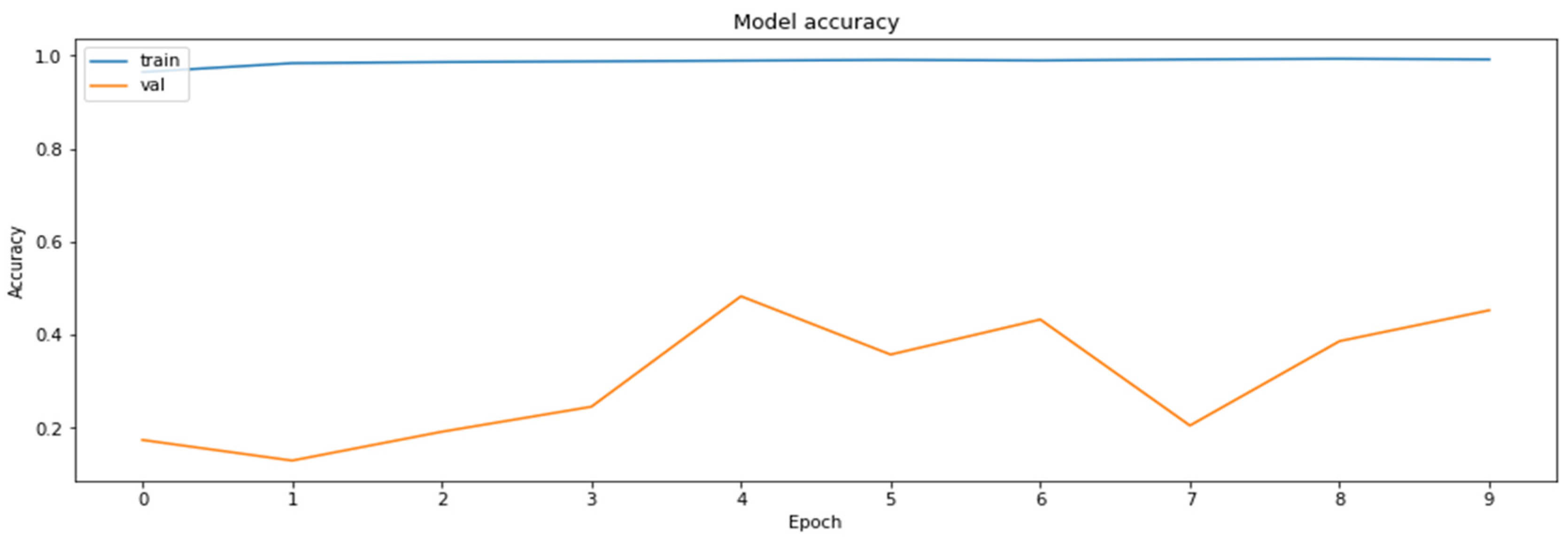
To determine the advantages of the model distillation, yet another MobileNetV2 model was also trained through a classical training process, during which the parameters were the same during the model compiling as those in the case of the base model. Training of this second MobileNetV2 model was carried out for the same number of epochs as was used for the duration of the distillation process. The results of the training of the second MobileNetV2 model are shown in Figure 15 and Figure 16.
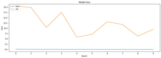
Figure 15.
The loss function values for the validation datasets obtained during the regular training of the model.
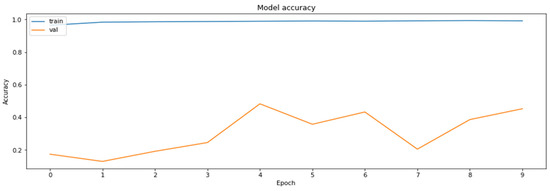
Figure 16.
The accuracy of the model for the validation datasets obtained during the regular training of the model.
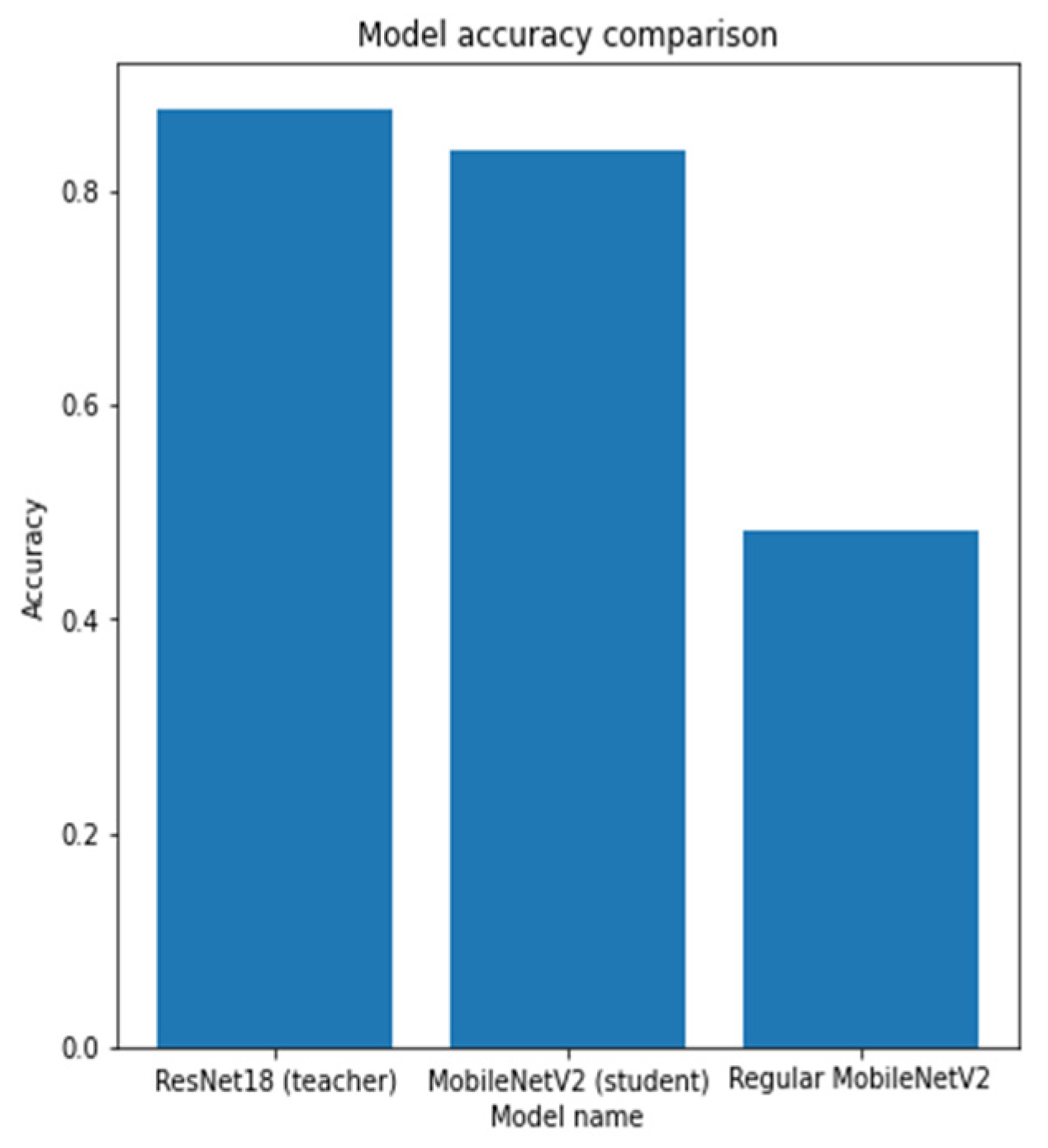
As can be seen according to the graphics, the accuracy of the regularly trained model did not reach the accuracy results achieved by the distilled model. Finally, the comparison of the accuracies of the two models for the validation dataset is shown in Figure 17.

Figure 17.
The comparison of the accuracy of the teacher model (the base ResNet18 model), the student model (MobileNetV2), and the regularly trained student model (MobileNetV2).
Given the fact that a larger number of the obtained models matched the application of one method (due to quantization), Table 2 shows the average time of the execution of a single training epoch for each of the methods.

Table 2.
The average time of the execution of a single training epoch for each of the methods.
Acronyms from Table 2:
- Base—initial ResNet18 model;
- PR—pruning method applied on the ResNet18 model;
- CL KPP 32—weight clustering, using KMeans++ for centroid initialization and 32 clusters applied on ResNet18 model;
- CL LIN 32—weight clustering, using linear centroid initialization and 32 clusters applied on the ResNet18 model;
- CL KPP 256—weight clustering, using KMeans++ for centroid initialization and 256 clusters applied on ResNet18 model;
- QAT—quantization-aware training applied on ResNet18 model;
- PCQAT PR—combined method, pruning part of the method applied on ResNet18 model;
- PCQAT CL—combined method, weight clustering part of the method applied on ResNet18 model;
- PCQAT QAT—combined method, quantization-aware training part of the method applied on ResNet18 model;
- Distillation—knowledge distillation of MobileNetV2 model from ResNet18 model.
4. Final Comparisons
The following characteristics of the obtained models were taken into consideration for the final comparison:
- The model execution time;
- The model accuracy;
- The model size;
- The model size after the zip-function-enabled compression.
The final comparison of the models was performed on a Raspberry Pi 4 device since TF Lite conversion generated the models optimized for ARM processors. Starting the models on processors with an x86 set of instructions generated drastically worse results concerning the model execution time for TF Lite-quantized models (they are so much worse in the case of INT8-quantized models that the evaluation process lasts for far too long). The platform on which the model was being executed had no influence on the remaining monitored model characteristics (the model accuracy and the model size). The validation set CRC-VAL-HE-7K was the dataset used for this final comparison.
4.1. The Model Execution Time
The total time needed for the model to classify all the images contained in the evaluation set was taken for the model comparison. The model comparison as per the execution time should be taken with caution since the models that are converted with the help of the TF Lite library are optimized for execution on ARM processors. It can be seen that the application of each compression method reduced the initial model execution time of 1409.98 s, whereas the TF Lite model conversion led to an increase in the execution time. The best results were obtained after the application of distillation, 670.22 s (since MobileNetV2 has three times as few parameters than ResNet18). Apart from distillation, significant results for the execution time were also achieved for the INT8 quantization of the models.
4.2. The Model Accuracy
Regarding accuracy, it can be seen that the application of pruning led to an accuracy loss of around 6%. The combination of pruning and integer quantization drastically degraded the performances of the models. The very transformation of the initial model in the TF Lite led to an accuracy loss of 10%, which can be used to present arguments for the same result (the same accuracy degradation) obtained after the application of quantization to the initial model. On the other hand, the models obtained with the help of QAT and the clustering of weights provided better results than the initial model. Where QAT is concerned, an improvement in the model accuracy of 4–6% was achieved, whereas that improvement was around 3–4% when speaking about weight clustering. These results show that it may be possible to train the base model, which would reach as much as 95% accuracy, or that the QAT and clustered models were overfitted for the selected validation subset. The application of the PCQAT technique degraded the model performances by 4–5%, which is correct bearing in mind the fact that this method led to the greatest model compression as per the size. The application of distillation led to a 4% accuracy loss.
4.3. The Model Size
The model size was the size of a model in the HDF5 format obtained with the help of the Keras save_model function or the tflite format in the case of the models converted with the help of the TF Lite library. What could be noticed is that the conversion of the models in the TF Lite reduced the size of the converted model about three times, that FP16 quantization reduced the model size two times, and INT8 reduced it four times to the initial TF Lite model. The distillation of the model, in this case, generated the best results, which generated the model size of almost 10 Mb (a compression of as many as 13 times was achieved).
4.4. The Model Size after the Zip-Function-Enabled Compression
The application of the zip compression to the obtained models led to a reduction in the file sizes with almost all the models, the best results simultaneously being obtained with the models compressed by pruning or the clustering of weights, with which this additional compression led to a reduction in the model size on the disk of 3.4 and 8.5 times, respectively (a reduction of 8.5 times was achieved in the case of the clustering of the weights with the linear initialization of the centroids). The combination of these two methods with the PCQAT-compressed model led to a compression of 3.4 times as well. The application of the zip function to the remaining models led to a reduction in the initial file by a few Mb, which can be neglected in the majority of the cases to the initial file size.
4.5. Recommendations for the Application of Compression with Tensorflow Library
The selection of a compression method depends on the model compression goal (i.e., what the primary compression goal is), the results of the existing models, as well as the platform on which the model will be executed. The simplest type of compression which is always applicable and does not require additional training is FP16 quantization (post-training). This type of quantization reduces the model size by one-half and leads to a faster model execution with Nvidia volt cards or the latest architecture because of the presence of a specialized piece of hardware for operations with FP16 data. For those reasons, it is sensible to apply this type of compression should the same significantly not degrade the original model’s performance. Should there be a need for the model to be applied on some microcomputers or should there be a need for the model to be used on Edge TPU devices (for example due to a reduced price for renting TPU cards to classical GPU cards), then INT8 quantization is what we have to resort to. The application of this quantization almost always requires that the QAT method be used before quantization itself so as not to witness any model performance degradation at all.
In the cases when the main goal is to reduce the model size on the disk (due to the transfer via a network), all the compression methods (pruning, quantization, and weight clustering) can be used.
The maximum compression can be achieved through a combination of a larger number of methods (such as PCQAT, for example). What we should be cautious about is the application of these methods to the key parts of a model (such as the model’s initial layers or the attention heads with the models using the attention mechanism).
In the cases when the main goal is to accelerate the model execution, the best to use is model quantization or model distillation. In situations such as these, distillation is always a sensible option, whereas quantization is only sensible if there is a specialized piece of hardware that will lead to acceleration while working with less-precise data. Should there be a group of trained models used together as an ensemble, the whole ensemble can be subjected to distillation onto one model, which drastically reduces that model’s size.
5. Conclusions
To enable a broader application of DNN models on RC devices, techniques intended to reduce their complexity need to be developed. As has already been seen in this paper, there are different DNN model compression technique groups, such as quantization, pruning, and parameter sharing. Model distillation is a special type of technique. With this technique, no existing model knowledge is reduced, but its knowledge is transferred onto a smaller model instead. A larger number of techniques need to be used at one time for the compression of bigger models. What can be concluded after the application of all these techniques is that contemporary DNN models are quite inefficient. The best results are obtained by training deeper and more complex models, whose compression or distillation reduces them to a more efficient model.
In this paper, quantization, pruning, weight clustering, QAT, PCQAT, and distillation were performed for the compression of ResNet18. The greatest model compression on the disk was achieved by applying the PCQAT method, whose application led to a reduction in the size of the initial model by as many as 45 times, whereas the greatest model acceleration was achieved by distillation on the MobileNetV2 model. Both methods lead to a reduction in the accuracy of the base model (around 4%). As has been stated, all the methods led to the compression of the initial size of the model with a slight loss in the model accuracy or an increase in the model accuracy. Therefore, in this case, better results cannot be achieved. Additionally, it might be interesting to explore whether the degradation of performance could be decreased by some other compression methods or by applying more sophisticated implementation of already mentioned methods.
All the methods led to the compression of the initial size of the model with a slight loss in the model accuracy or an increase in the model accuracy in the case of QAT and weight clustering.
In addition, the distillation process may further be improved by introducing the teacher-teaching assistant model, whose complexity ranges between ResNet18 and MobileNetV2, or distillation could be performed with the help of hints. Additionally, application of evolutionary algorithms [43] and multicriteria decision making [44] can be investigated for compressing DNNs.
Author Contributions
Conceptualization, B.P., U.V. and D.K.; methodology, M.S. and D.S.; software, B.P.; writing—original draft preparation, B.P., U.V. and D.K.; writing—review and editing, M.S. and D.S.; supervision, D.K. All authors have read and agreed to the published version of the manuscript.
Funding
This research received no external funding.
Data Availability Statement
Not applicable.
Conflicts of Interest
The authors declare no conflict of interest.
Appendix A
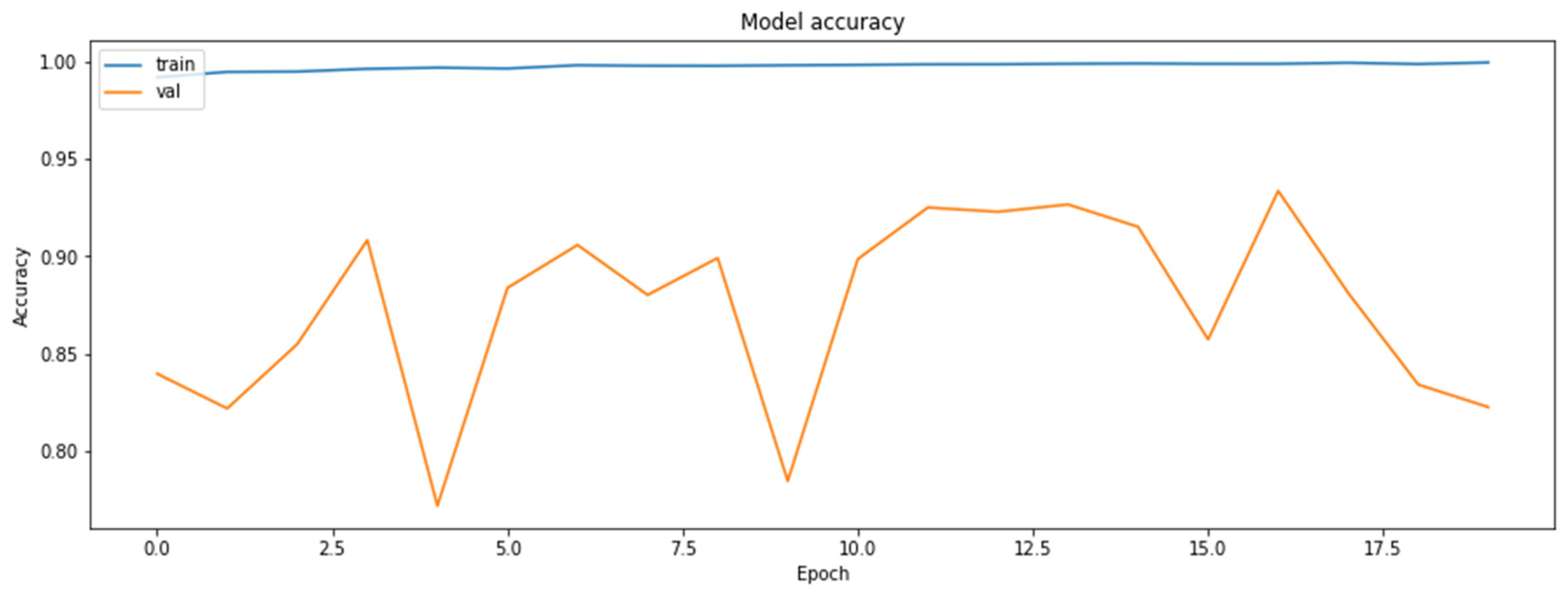
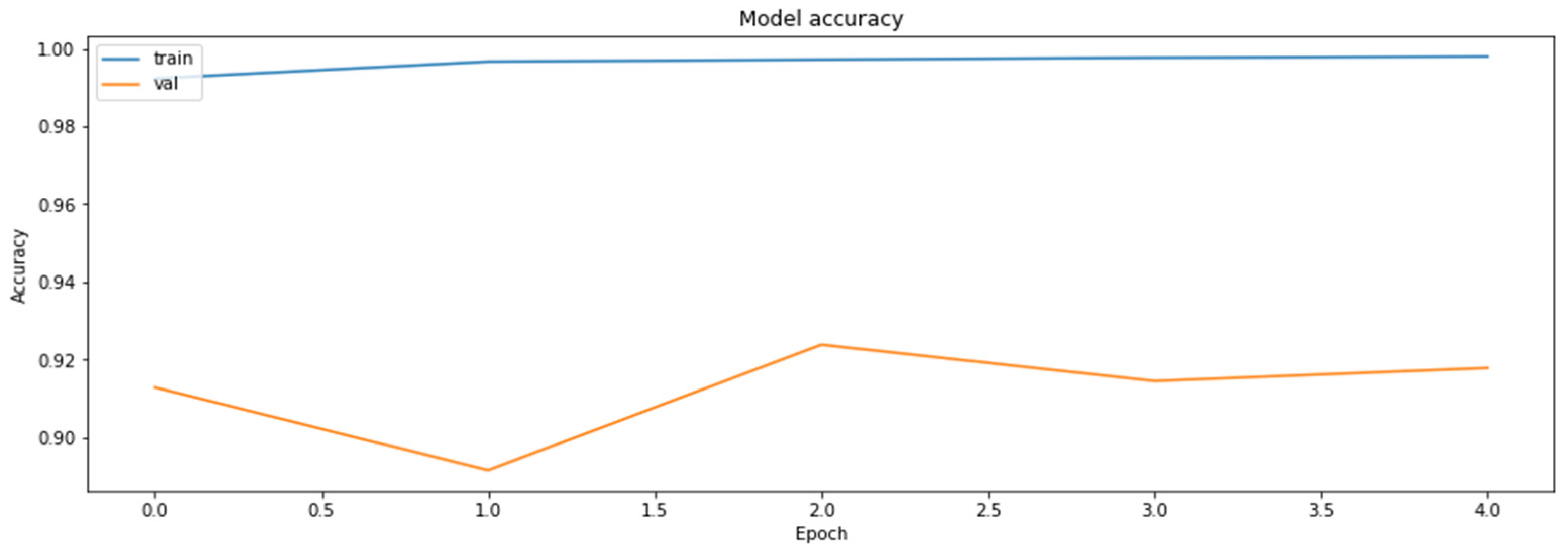
A couple of combinations of the number of clusters and the centroid initialization algorithm were tested. A review of the model training results is given in Figure A1, Figure A2, Figure A3, Figure A4, Figure A5, Figure A6 and Figure A7.
The centroid initialization algorithm: KMeans++
The number of the clusters: 32
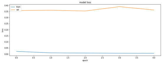
Figure A1.
The loss function value for the training and the validation datasets obtained during the training of the model with the weights clustered with the KMeans++ initialization of 32 centroids.
Figure A1.
The loss function value for the training and the validation datasets obtained during the training of the model with the weights clustered with the KMeans++ initialization of 32 centroids.
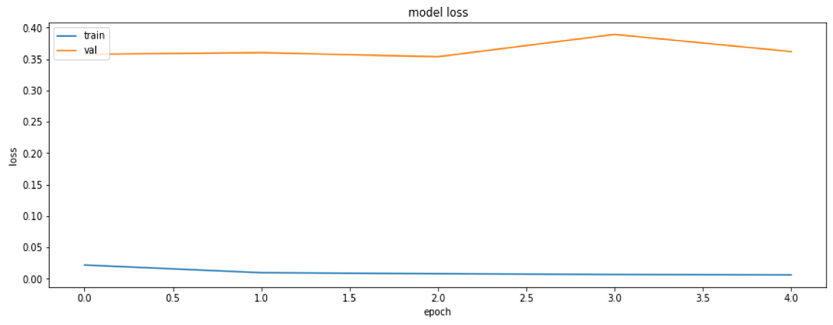
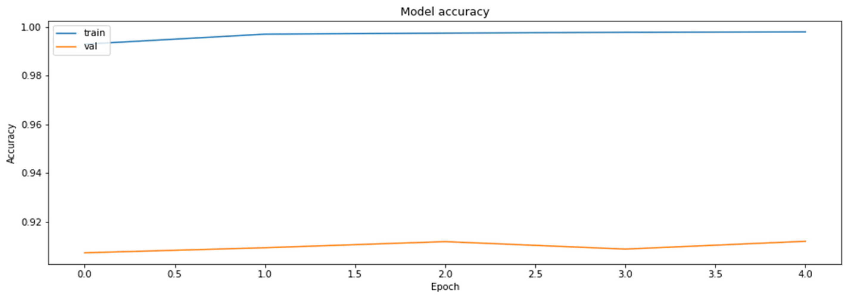
Figure A2.
The accuracy of the model for the training and the validation dataset obtained during the training of the model with the weights clustered with KMeans++ initialization of 32 centroids.
Figure A2.
The accuracy of the model for the training and the validation dataset obtained during the training of the model with the weights clustered with KMeans++ initialization of 32 centroids.
The centroid initialization algorithm: Linear
The number of the clusters: 32
Figure A3.
The loss function values for the training and the validation datasets obtained during the training of the model with the weights clustered with the linear initialization of 32 centroids.
Figure A3.
The loss function values for the training and the validation datasets obtained during the training of the model with the weights clustered with the linear initialization of 32 centroids.
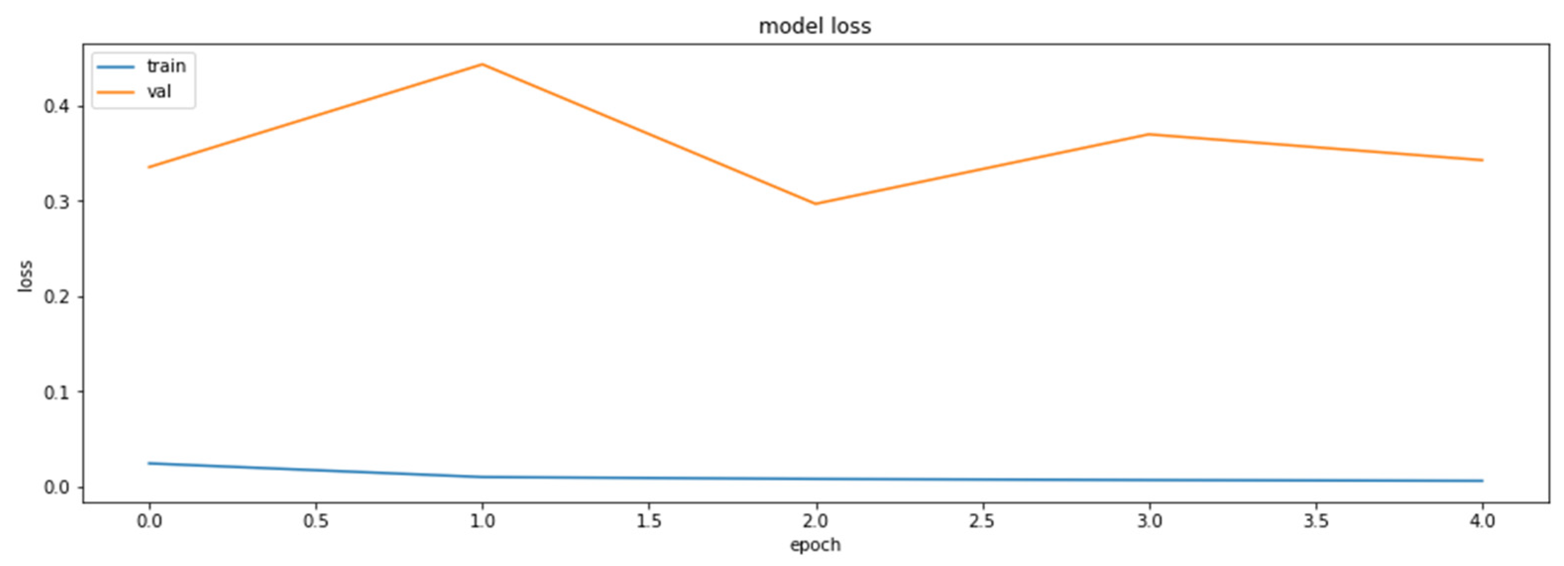
Figure A4.
The accuracy of the model for the training and the validation datasets obtained during the training of the model with the weights clustered with the linear initialization of 32 centroids.
Figure A4.
The accuracy of the model for the training and the validation datasets obtained during the training of the model with the weights clustered with the linear initialization of 32 centroids.
The centroid initialization algorithm: KMeans++
The number of the clusters: 256
Figure A5.
The loss function value for the training and the validation datasets obtained during the training of the model with the weights clustered with KMeans++ initialization of 256 centroids.
Figure A5.
The loss function value for the training and the validation datasets obtained during the training of the model with the weights clustered with KMeans++ initialization of 256 centroids.
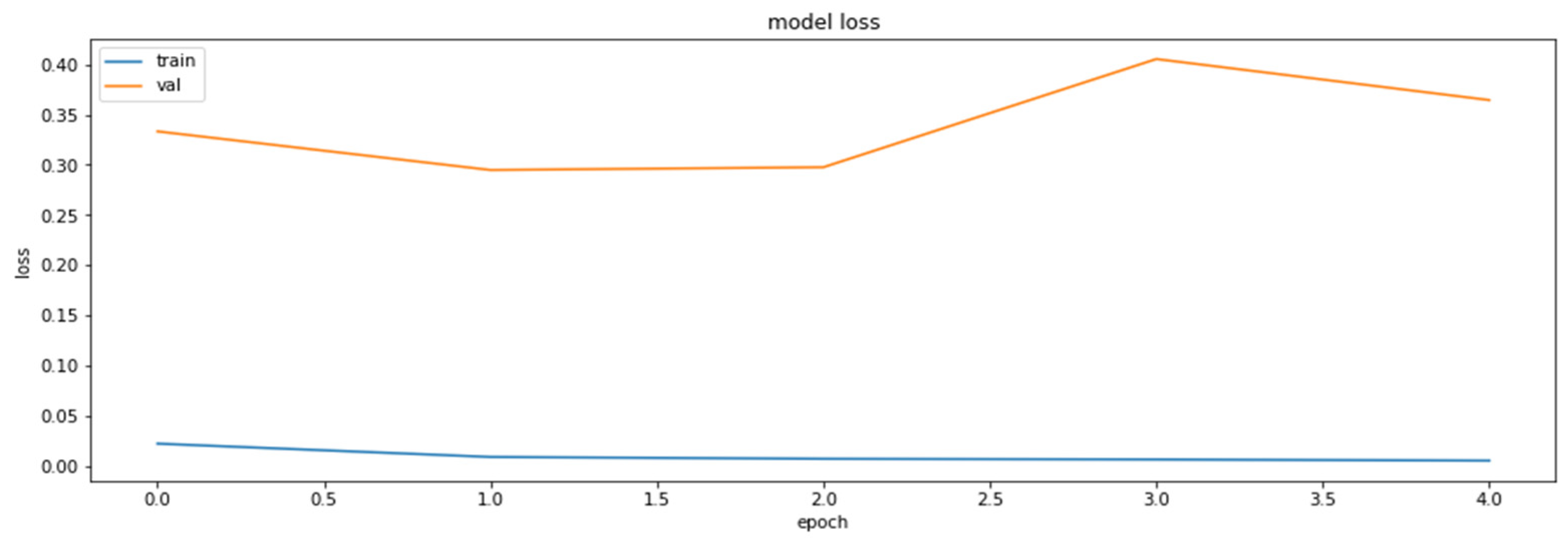

Figure A6.
The accuracy of the model for the training and the validation datasets obtained during the training of the model with the weights clustered with KMeans++ initialization of 256 centroids.
Figure A6.
The accuracy of the model for the training and the validation datasets obtained during the training of the model with the weights clustered with KMeans++ initialization of 256 centroids.

Further in the text, the results of the comparison(s) of the obtained models are presented (see Figure A7 and Figure A8). The models that were created using the same compression method are colored with the same color. The colors are as follows:


Figure A7.
The comparison of the model accuracies and the comparison of the model execution time.
Figure A7.
The comparison of the model accuracies and the comparison of the model execution time.
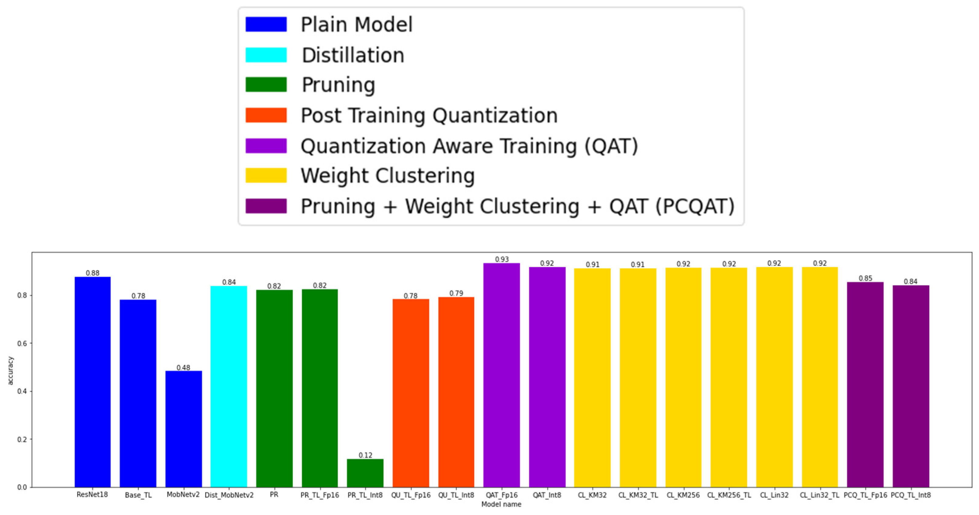

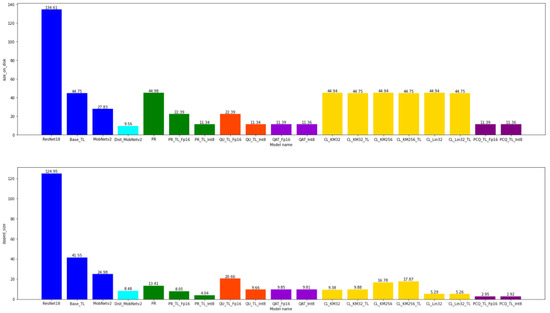
Figure A8.
The comparison of the model size on the disk and the comparison of the model size on the disk after the application of the zip function.
Figure A8.
The comparison of the model size on the disk and the comparison of the model size on the disk after the application of the zip function.

References
- Kotenko, I.; Izrailov, K.; Buinevich, M. Static Analysis of Information Systems for IoT Cyber Security: A Survey of Machine Learning Approaches. Sensors 2022, 22, 1335. [Google Scholar] [CrossRef] [PubMed]
- Shenbagalakshmi, V.; Jaya, T. Application of machine learning and IoT to enable child safety at home environment. J. Supercomput. 2022, 78, 10357–10384. [Google Scholar] [CrossRef]
- Mohammadi, F.G.; Shenavarmasouleh, F.; Arabnia, H.R. Applications of Machine Learning in Healthcare and Internet of Things (IOT): A Comprehensive Review. arXiv 2022, arXiv:2202.02868. [Google Scholar]
- Mohammed, C.M.; Askar, S. Machine learning for IoT healthcare applications: A review. Int. J. Sci. Bus. 2021, 5, 42–51. [Google Scholar]
- Hamad, Z.J.; Askar, S. Machine Learning Powered IoT for Smart Applications. Int. J. Sci. Bus. 2021, 5, 92–100. [Google Scholar]
- Atul, D.J.; Kamalraj, R.; Ramesh, G.; Sankaran, K.S.; Sharma, S.; Khasim, S. A machine learning based IoT for providing an intrusion detection system for security. Microprocess. Microsyst. 2021, 82, 103741. [Google Scholar] [CrossRef]
- Murdoch, W.J.; Singh, C.; Kumbier, K.; Abbasi-Asl, R.; Yu, B. Definitions, methods, and applications in interpretable machine learning. Proc. Natl. Acad. Sci. USA 2019, 116, 22071–22080. [Google Scholar] [CrossRef] [Green Version]
- Chen, R.-C.; Dewi, C.; Huang, S.-W.; Caraka, R.E. Selecting critical features for data classification based on machine learning methods. J. Big Data 2020, 7, 1–26. [Google Scholar] [CrossRef]
- Abdulhammed, R.; Musafer, H.; Alessa, A.; Faezipour, M.; Abuzneid, A. Features dimensionality reduction ap-proaches for machine learning based network intrusion detection. Electronics 2019, 8, 322. [Google Scholar] [CrossRef] [Green Version]
- Murdoch, W.J.; Singh, C.; Kumbier, K.; Abbasi-Asl, R.; Yu, B. Interpretable machine learning: Definitions, methods, and applications. arXiv 2019, arXiv:1901.04592. [Google Scholar] [CrossRef] [Green Version]
- Helm, J.M.; Swiergosz, A.M.; Haeberle, H.S.; Karnuta, J.M.; Schaffer, J.L.; Krebs, V.E.; Spitzer, A.I.; Ramkumar, P.N. Machine Learning and Artificial Intelligence: Definitions, Applications, and Future Directions. Curr. Rev. Musculoskelet. Med. 2020, 13, 69–76. [Google Scholar] [CrossRef] [PubMed]
- Canziani, A.; Paszke, A.; Culurciello, E. An analysis of deep neural network models for practical applications. arXiv 2016, arXiv:1605.07678. [Google Scholar]
- Sze, V.; Chen, Y.-H.; Yang, T.-J.; Emer, J.S. Efficient Processing of Deep Neural Networks: A Tutorial and Survey. Proc. IEEE 2017, 105, 2295–2329. [Google Scholar] [CrossRef] [Green Version]
- Anbarasan, M.; Muthu, B.; Sivaparthipan, C.; Sundarasekar, R.; Kadry, S.; Krishnamoorthy, S.; Dasel, A.A. Detection of flood disaster system based on IoT, big data and convolutional deep neural network. Comput. Commun. 2020, 150, 150–157. [Google Scholar] [CrossRef]
- Han, S.; Mao, H.; Dally, W.J. Deep compression: Compressing deep neural networks with pruning, trained quantization and Huffman coding. arXiv 2015, arXiv:1510.00149. [Google Scholar]
- Lakhan, A.; Mastoi, Q.-U.; Elhoseny, M.; Memon, M.S.; Mohammed, M.A. Deep neural network-based application partitioning and scheduling for hospitals and medical enterprises using IoT assisted mobile fog cloud. Enterp. Inf. Syst. 2021, 15, 1–23. [Google Scholar] [CrossRef]
- Sattler, F.; Wiegand, T.; Samek, W. Trends and advancements in deep neural network communication. arXiv 2020, arXiv:2003.03320. [Google Scholar]
- Verhelst, M.; Moons, B. Embedded Deep Neural Network Processing: Algorithmic and Processor Techniques Bring Deep Learning to IoT and Edge Devices. IEEE Solid-State Circuits Mag. 2017, 9, 55–65. [Google Scholar] [CrossRef]
- Mehra, M.; Saxena, S.; Sankaranarayanan, S.; Tom, R.J.; Veeramanikandan, M. IoT based hydroponics system using Deep Neural Networks. Comput. Electron. Agric. 2018, 155, 473–486. [Google Scholar] [CrossRef]
- Thakkar, A.; Chaudhari, K. A comprehensive survey on deep neural networks for stock market: The need, challenges, and future directions. Expert Syst. Appl. 2021, 177, 114800. [Google Scholar] [CrossRef]
- Brajević, I.; Brzaković, M.; Jocić, G. Solving integer programming problems by using population-based beetle antennae search algorithm. J. Process Manag. New Technol. 2021, 9, 89–99. [Google Scholar] [CrossRef]
- Abdou, M.A. Literature review: Efficient deep neural networks techniques for medical image analysis. Neural Comput. Appl. 2022, 34, 5791–5812. [Google Scholar] [CrossRef]
- Fang, X.; Liu, H.; Xie, G.; Zhang, Y.; Liu, D. Deep Neural Network Compression Method Based on Product Quantization. In Proceedings of the 39th Chinese Control Conference (CCC), Shenyang, China, 27–30 July 2020. [Google Scholar] [CrossRef]
- Anwar, S.; Hwang, K.; Sung, W. Structured Pruning of Deep Convolutional Neural Networks. ACM J. Emerg. Technol. Comput. Syst. 2017, 13, 1–18. [Google Scholar] [CrossRef] [Green Version]
- Li, H.; Kadav, A.; Durdanovic, I.; Samet, H.; Graf, H.P. Pruning Filters for Efficient ConvNets. arXiv 2016, arXiv:1608.08710. [Google Scholar]
- Chen, W.; Wilson, J.T.; Tyree, S.; Weinberger, K.Q.; Chen, Y. Compressing Neural Networks with the Hashing Trick. In Proceedings of the 32nd International Conference on Machine Learning, Lille, France, 6–11 July 2015. [Google Scholar]
- Hinton, G.; Vinyals, O.; Dean, J. Distilling the Knowledge in a Neural Network. arXiv 2015, arXiv:1503.02531. [Google Scholar]
- Bucila, C.; Caruana, R.; Niculescu-Mizil, A. Model compression. In Proceedings of the 12th ACM SIGKDD International Conference on Knowledge Discovery and Data Mining, KDD ’06, New York, NY, USA, 20–23 August 2006; ACM: New York, NY, USA; pp. 535–541. [Google Scholar]
- Gou, J.; Yu, B.; Maybank, S.J.; Tao, D. Knowledge Distillation: A Survey. Int. J. Comput. Vis. 2021, 129, 1789–1819. [Google Scholar] [CrossRef]
- Cai, H.; Gan, C.; Wang, T.; Zhang, Z.; Han, S. Once-for-All: Train One Network and Specialize It for Efficient Deployment. arXiv 2019, arXiv:1908.09791. [Google Scholar]
- Luo, J.-H.; Wu, J.; Lin, W. ThiNet: A Filter Level Pruning Method for Deep Neural Network Compression. In Proceedings of the IEEE International Conference on Computer Vision (ICCV), Venice, Italy, 22–29 October 2017; Institute of Electrical and Electronics Engineers (IEEE): Piscataway, NJ, USA, 2017; pp. 5068–5076. [Google Scholar]
- Duan, X.; Guo, D.; Qin, C. Image Information Hiding Method Based on Image Compression and Deep Neural Network. Comput. Model. Eng. Sci. 2020, 124, 721–745. [Google Scholar] [CrossRef]
- Chen, R.; Chen, Y.; Su, J. Deep convolutional neural networks compression method based on linear representation of kernels. In Proceedings of the Eleventh International Conference on Machine Vision (ICMV 2018), Munich, Germany, 30 November 2018; 11041, p. 110412N. [Google Scholar] [CrossRef]
- Sun, S.; Chen, W.; Bian, J.; Liu, X.; Liu, T. Ensemble-Compression: A New Method for Parallel Training of Deep Neural Networks. Machine Learning and Knowledge Discovery in Databases. In Lecture Notes in Artificial Intelligence; ECML PKDD 2017, PT I; Book Series; Volume 10534, pp. 187–202. [CrossRef] [Green Version]
- Salehinejad, H.; Valaee, S. Ising-dropout: A Regularization Method for Training and Compression of Deep Neural Networks. In Proceedings of the ICASSP IEEE International Conference on Acoustics, Speech and Signal Processing (ICASSP), Brighton, UK, 12–17 May 2019; pp. 3602–3606. [Google Scholar] [CrossRef] [Green Version]
- Yamagiwa, S.; Yang, W.; Wada, K. Adaptive Lossless Image Data Compression Method Inferring Data Entropy by Applying Deep Neural Network. Electronics 2022, 11, 504. [Google Scholar] [CrossRef]
- Zeng, L.; Chen, S.; Zeng, S. An Efficient End-to-End Channel Level Pruning Method for Deep Neural Networks Compression. In Proceedings of the IEEE 10th International Conference on Software Engineering and Service Science (ICSESS), Beijing, China, 18–20 October 2019; pp. 43–46. [Google Scholar] [CrossRef]
- Ademola, O.A.; Leier, M.; Petlenkov, E. Evaluation of Deep Neural Network Compression Methods for Edge Devices Using Weighted Score-Based Ranking Scheme. Sensors 2021, 21, 7529. [Google Scholar] [CrossRef]
- Kather, J.N.; Halama, N.; Marx, A. Zenodo. Available online: https://zenodo.org/record/1214456#.YZkx57so9hF (accessed on 12 December 2021).
- Macenko, M.; Niethammer, M.; Marron, J.S.; Borland, D.; Woosley, J.T.; Guan, X.; Schmitt, C.; Thomas, N.E. A Method For Normalizing Histology Slides For Quantitative Analysis. In Proceedings of the IEEE International Symposium on Biomedical Imaging, Boston, MA, USA, 28 June–1 July 2009. [Google Scholar]
- Yakubovskiy, P. Classification Models Zoo—Keras (and TensorFlow Keras). Available online: https://pypi.org/project/image-classifiers (accessed on 12 December 2021).
- TensorFlow Model Optimization Toolkit. Available online: https://www.tensorflow.org/model_optimization/guide (accessed on 3 May 2022).
- Zhou, Y.; Yen, G.G.; Yi, Z. A Knee-Guided Evolutionary Algorithm for Compressing Deep Neural Networks. IEEE Trans. Cybern. 2019, 51, 1626–1638. [Google Scholar] [CrossRef] [PubMed]
- dos Santos, M.; Costa, I.P.d.A.; Gomes, C.F.S. Multicriteria decision-making in the selection of warships: A new approach to the ahp method. Int. J. Anal. Hierarchy Process 2021, 13, 147–169. [Google Scholar] [CrossRef]
Publisher’s Note: MDPI stays neutral with regard to jurisdictional claims in published maps and institutional affiliations. |
© 2022 by the authors. Licensee MDPI, Basel, Switzerland. This article is an open access article distributed under the terms and conditions of the Creative Commons Attribution (CC BY) license (https://creativecommons.org/licenses/by/4.0/).

