
An Adaptive Three-Dimensional Improved Virtual Force Coverage Algorithm for Nodes in WSN


Abstract
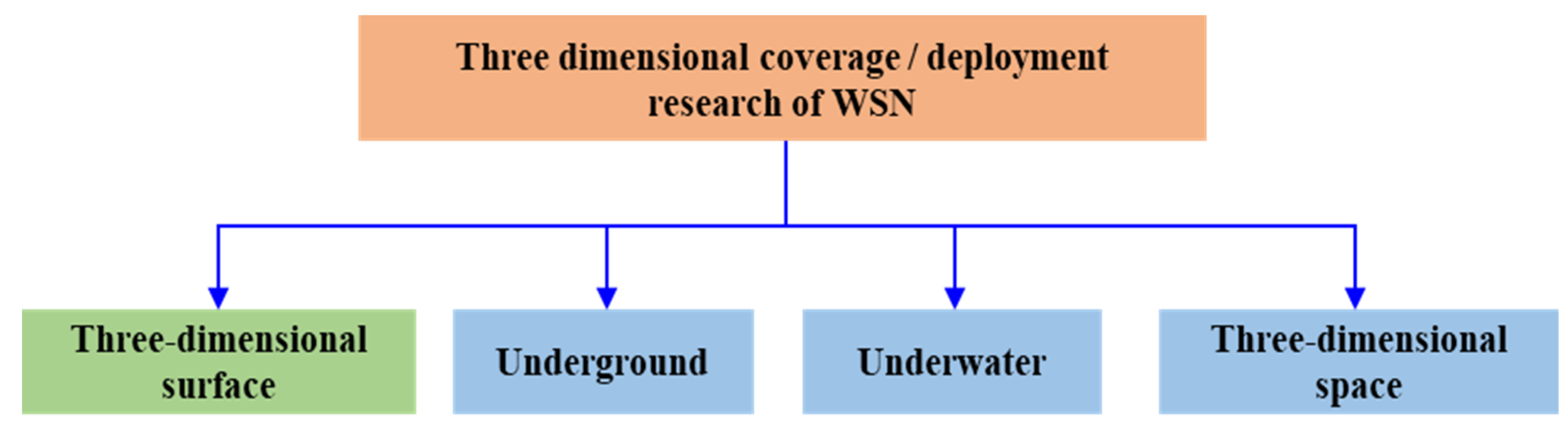
:1. Introduction
2. Coverage Problem in Three-Dimensional Space
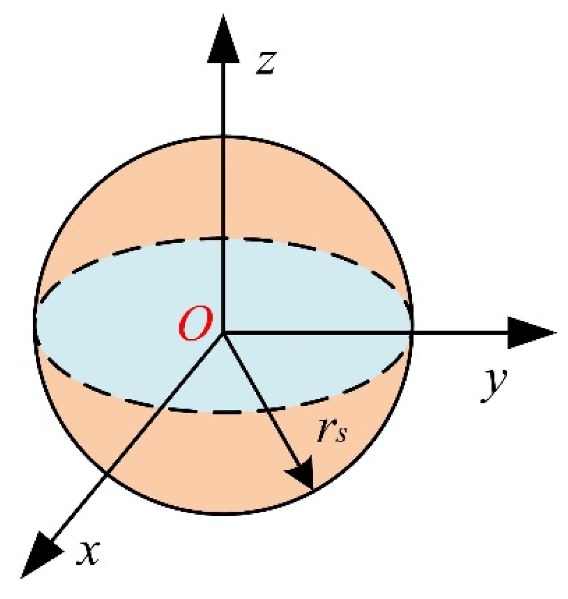
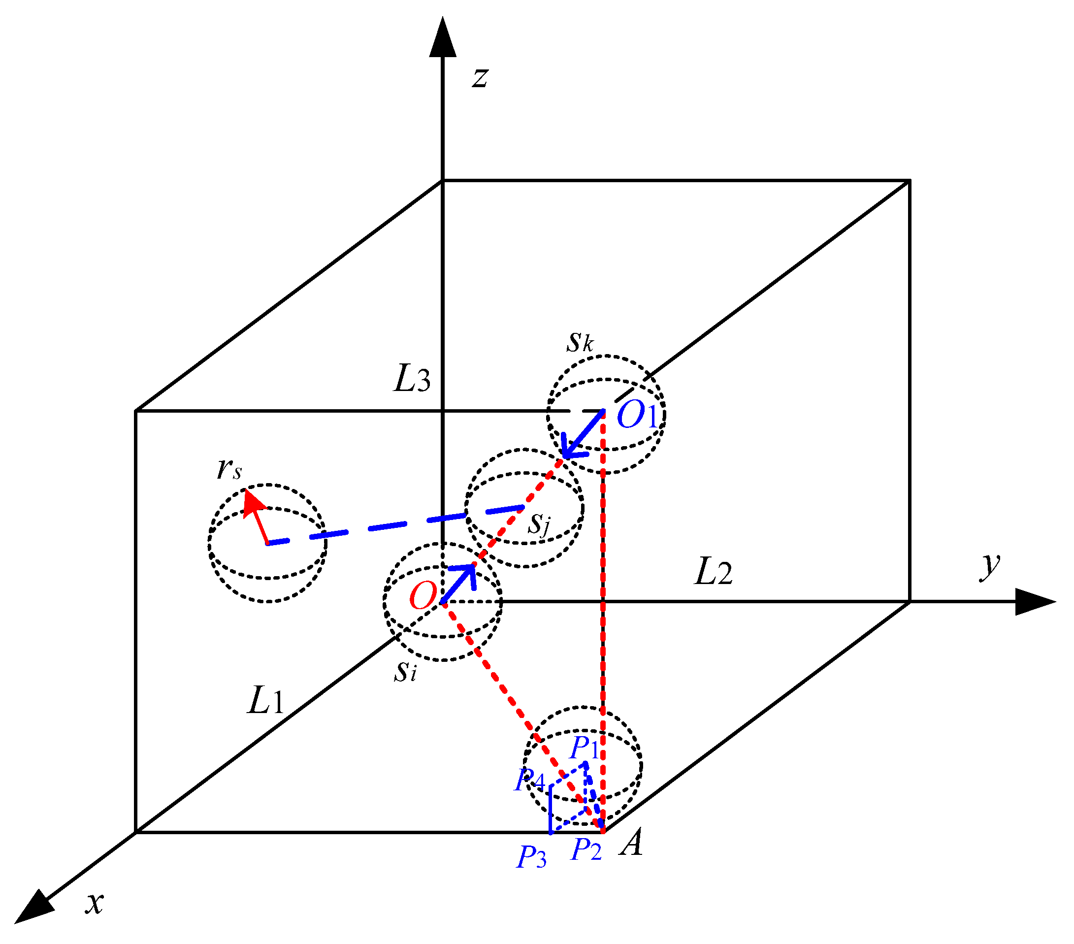
2.1. Node Perception Model
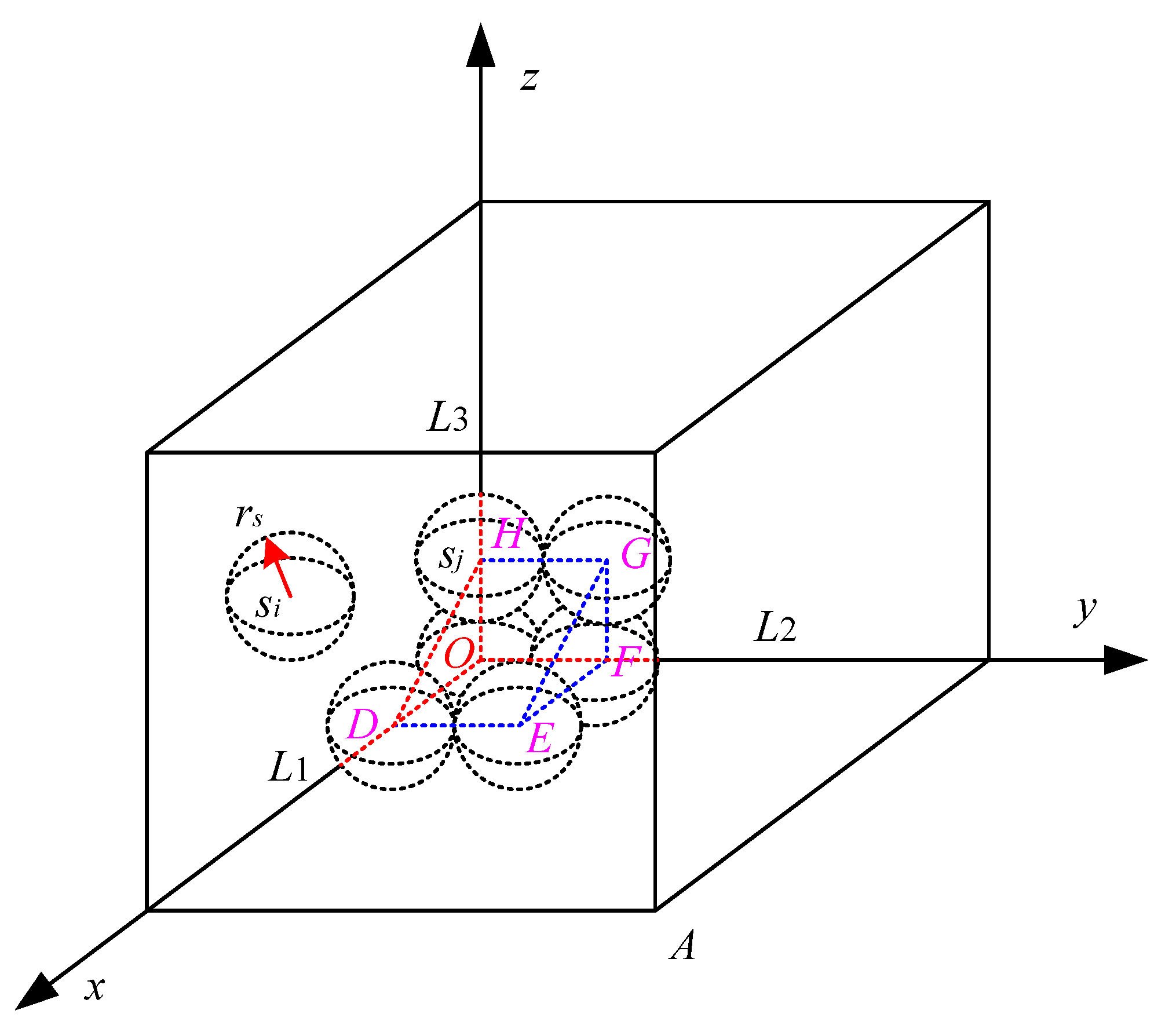
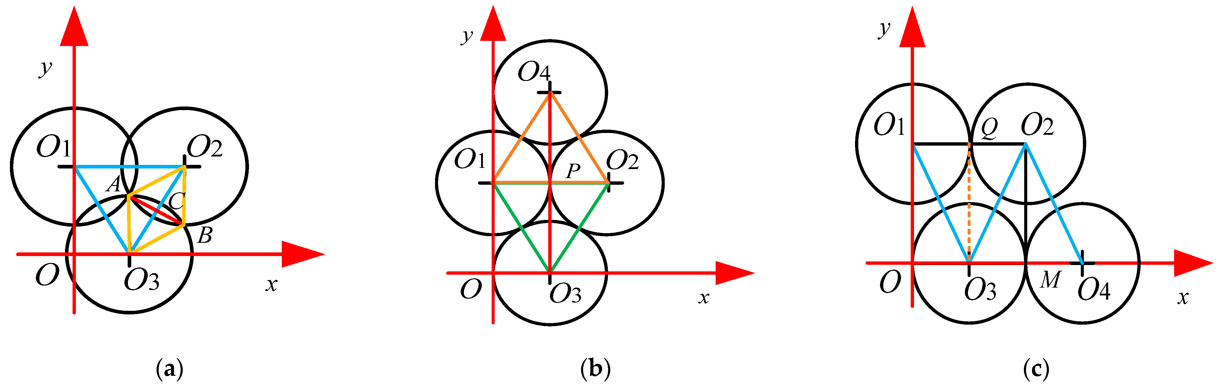
2.2. Three-Dimensional Point Coverage
2.3. Three-Dimensional Coverage Rate
3. Three-Dimensional Improved Virtual Force Coverage (3D-IVFC) Algorithm
3.1. Node Initial Position
3.2. Virtual Force Resultant Force
3.2.1. Force between Nodes
3.2.2. Area Boundary Limitation
3.3. Node Mobility Strategy
3.4. Adaptive Virtual Force Parameters
3.5. Complexity Analysis
| Algorithm 1: Pseudo-code of the 3D-IVFC algorithm. |
| Input: Monitoring area 500 m × 500 m × 500 m, the coordinate position of the node, and the maximum iterations Max_iter. |
| 1. Set the scope of the three-dimensional space area: Xmax = 500, Xmin = 10; Ymax = 500, Ymin = 10; Zmax = 500, Zmin = 10, and the step length of the point to be monitored is 25. |
| 2. Randomly deploy the initial position of nodes, and calculate coverage and unmonitored points k. |
| 3. For t = 1: Max_iter |
| 4. For i = 1: n |
| 5. For k = 1: k |
| 6. Calculate the distance between the node and the unmonitored point using Equation (2). |
| 7. If dik > rs |
| 8. Update the parameters using Equation (26). |
| 9. Calculate the resultant force F using Equations (13), (15)–(17). |
| 10. End |
| 11. End |
| 12. Move the node in space using Equations (18)–(20). |
| 13. End |
| 14. For i = 1: n |
| 15. For j = 1: n |
| 16. Calculate the distance between nodes using Equation (2). |
| 17. If dik > rs and dik < = rc |
| 18. Calculate the resultant force F using Equations (13), (15)–(17). |
| 19. End |
| 20. End |
| 21. Update the position of the node in space using Equations (18)–(20). |
| 22. Determine whether the node location exceeds the deployed space. |
| 23. End |
| 24. Update the coverage. |
| 25. End |
| Output: Optimized coverage, node location, and node movement trajectory |
4. Simulation Results
4.1. Experimental Environment and Parameter Setting
4.2. Different Initial Deployment Strategies
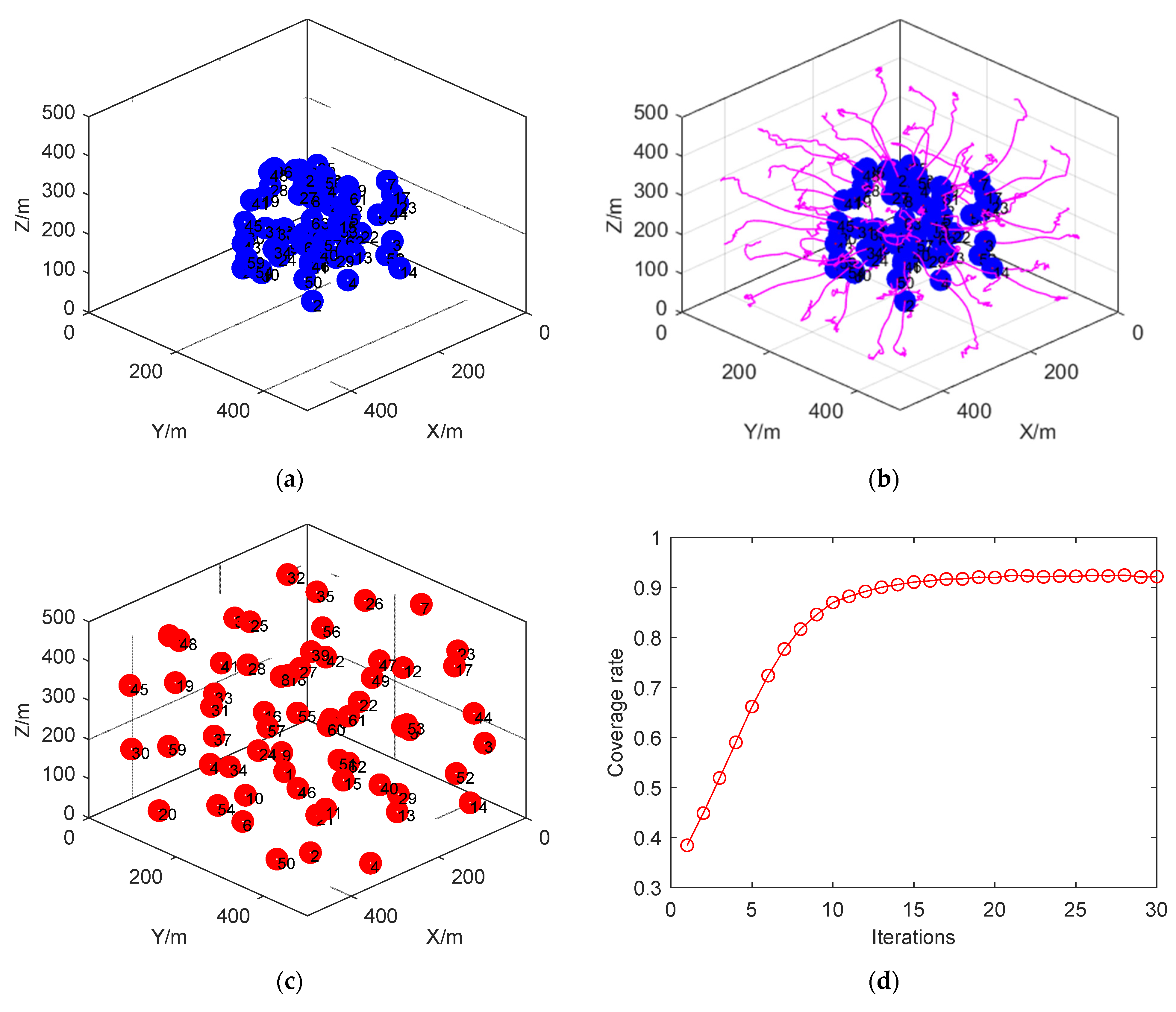
4.2.1. Case 1: Initial Node Random Deployment (3D-IVFC Algorithm)
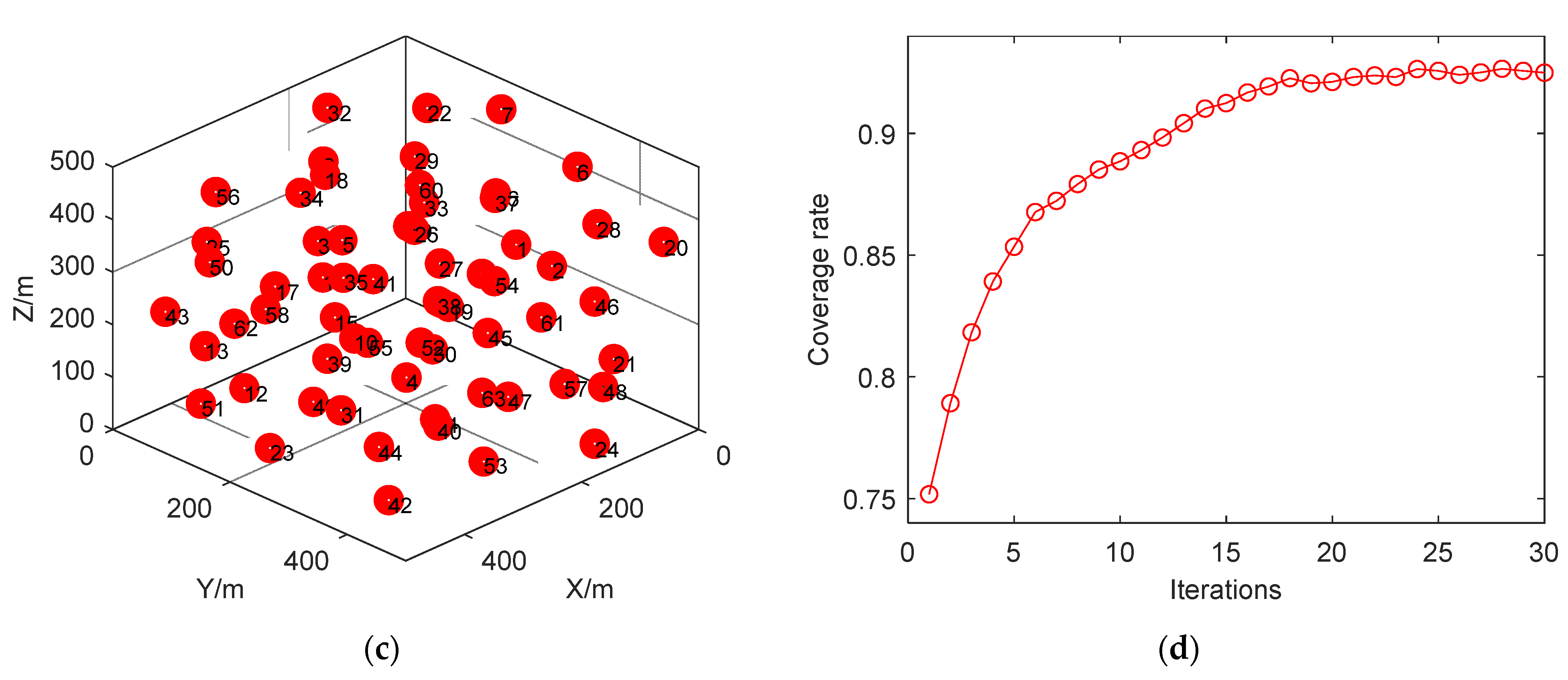
4.2.2. Case 2: Initial Node Location Centered Deployment (3D-IVFC Algorithm)
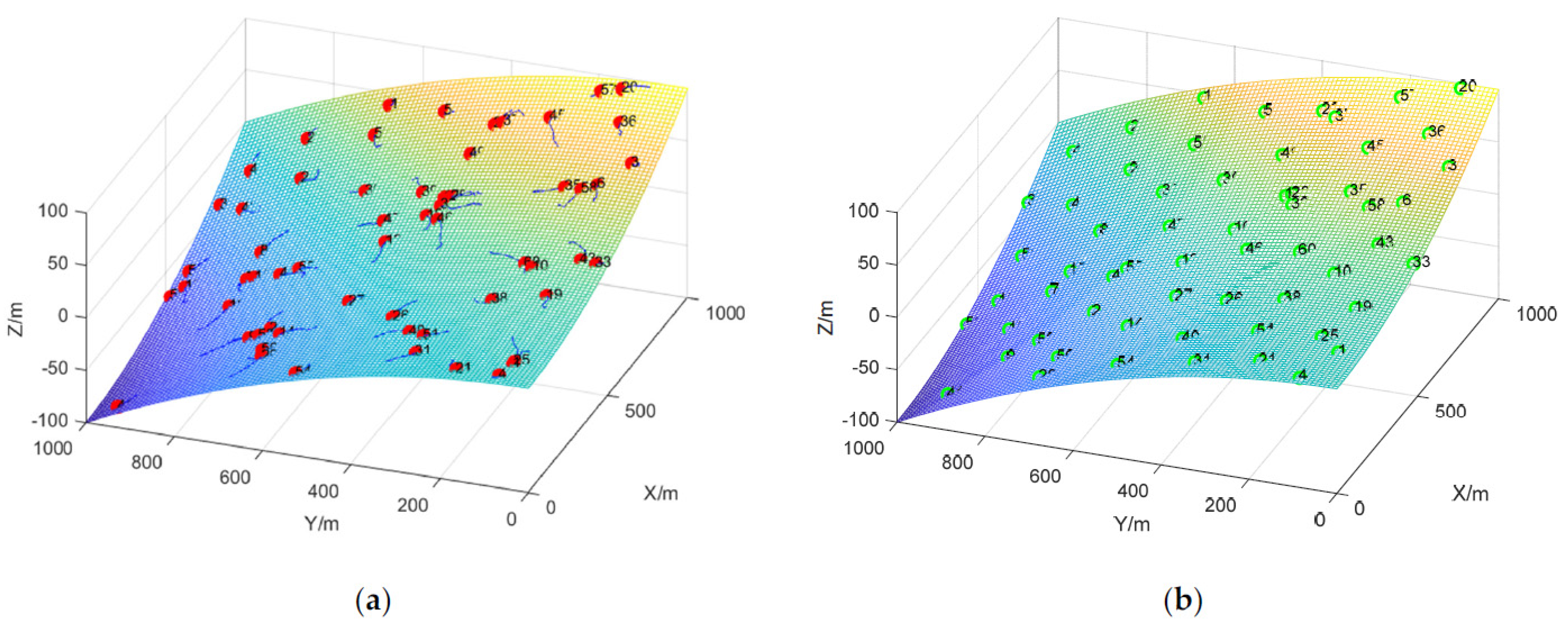
4.2.3. D-VFC Algorithm for the Surface Coverage Issue
5. Discussion
6. Conclusions
Author Contributions
Funding
Institutional Review Board Statement
Informed Consent Statement
Data Availability Statement
Conflicts of Interest
References
- Akyildiz, I.F.; Su, W.; Sankarasubram-Aniam, Y.; Cayirci, E. Wireless sensor networks: A survey. Comput. Netw. 2002, 38, 393–422. [Google Scholar] [CrossRef] [Green Version]
- Rashid, B.; Rehmani, M.H. Applications of wireless sensor networks for urban areas: A survey. J. Netw. Comput. Appl. 2016, 60, 192–219. [Google Scholar] [CrossRef]
- Akyildiz, I.F.; Pompili, D.; Melodia, T. Underwater acoustic sensor networks: Research challenges. Ad Hoc Netw. 2005, 3, 257–279. [Google Scholar] [CrossRef]
- Akyildiz, I.F.; Stuntebeck, E.P. Wireless underground sensor networks: Research challenges. Ad Hoc Netw. 2006, 4, 669–686. [Google Scholar] [CrossRef]
- Huang, C.F.; Tseng, Y.; Lo, L.C. The coverage problem in three-dimensional wireless sensor networks. In Proceedings of the IEEE Global Telecommunications Conference, Globecom’04, Dallas, TX, USA, 29 November–3 December 2004; pp. 3182–3186. [Google Scholar]
- Watfa, M.K.; Commuri, S. The 3-dimensional wireless sensor network coverage problem. In Proceedings of the IEEE International Conference on Networking, Sensing and Control, Ft. Lauderdale, FL, USA, 23–25 April 2006; pp. 856–861. [Google Scholar]
- Zhao, M.; Lei, J.; Lei, J.; Wu, M.Y.; Liu, Y.; Shu, W. Surface coverage in wireless sensor networks. In Proceedings of the IEEE INFOCOM, Rio de Janeiro, Brazil, 19–25 April 2009; pp. 109–117. [Google Scholar]
- Zafer, M.; Senouci, M.R.; Aissani, M. Efficient deployment approach of wireless sensor networks on 3D terrains. Int. J. Data Min. Model. Manag. 2021, 13, 114–136. [Google Scholar] [CrossRef]
- Bai, X.; Zhang, C.; Xuan, D.; Jia, W. Full-coverage and k-connectivity (k=14,6) three dimensional networks. In Proceedings of the IEEE INFOCOM, Rio de Janeiro, Brazil, 19–25 April 2009; pp. 388–396. [Google Scholar]
- Si, P.; Ma, J.; Tao, F.; Fu, Z.; Shu, L. Energy-efficient barrier coverage with probabilistic sensors in wireless sensor networks. IEEE Sens. J. 2020, 20, 5624–5633. [Google Scholar] [CrossRef]
- Saad, A.; Senouci, M.R.; Benyattou, O. Toward a realistic approach for the deployment of 3D Wireless Sensor Networks. IEEE Trans. Mob. Comput. 2022, 21, 1508–1519. [Google Scholar] [CrossRef]
- Ammari, H.M.; Das, S.K. A study of k-coverage and measures of connectivity in 3D wireless sensor networks. IEEE Trans. Comput. 2010, 59, 243–257. [Google Scholar] [CrossRef]
- Zhong, Y.X.; Huang, J.G.; Han, J. Research on deployment, coverage and connectivity in three- dimensional sensor networks. Control Decis. 2011, 26, 1447–1451. [Google Scholar]
- Boukerche, A.; Sun, P. Connectivity and coverage-based protocols for wireless sensor networks. Ad Hoc Netw. 2018, 80, 54–69. [Google Scholar] [CrossRef]
- Liu, H.; Chai, Z.J.; Du, J.Z.; Wu, B. Sensor redeployment algorithm based on combined virtual forces in three-dimensional space. Acta Autom. Sin. 2011, 37, 713–723. [Google Scholar]
- Tan, L.; Wang, Y.H.; Yang, M.H.; Hu, J.P.; Yang, C.Y. Three-dimensional space self-deployment algorithm based on virtual force compensation. Chin. J. Sci. Instrum. 2015, 36, 2570–2578. [Google Scholar]
- Tang, X.J.; Tan, L.; Wang, M.J. Autonomous deployment algorithm of three-dimensional mobile sensor network based on Voronoi diagram. Chin. J. Sens. Actuators 2018, 31, 613–619. [Google Scholar]
- Chen, Y.; Cao, L.Z. Virtual potential field and learning automata-based coverage control algorithm for directional sensor networks. Syst. Eng. Electron. 2015, 37, 1177–1184. [Google Scholar] [CrossRef]
- Zou, Y.; Chakrabarty, K. Sensor deployment and target localization based on virtual forces. In Proceedings of the IEEE INFOCOM, San Francisco, CA, USA, 30 March–3 April 2003; pp. 1293–1303. [Google Scholar]
- Liu, X.; Wang, X.; Jia, J.; Huang, M. A distributed deployment algorithm for communication coverage in wireless robotic networks. J. Netw. Comput. Appl. 2021, 180, 103019. [Google Scholar] [CrossRef]
- Hu, T.; Zhong, S. Research on a virtual force algorithm in Wireless Sensor Network. In Proceedings of the International Conference on Frontiers of Electronics, Information and Computation Technologies, Changsha, China, 21–23 May 2021; pp. 1–5. [Google Scholar]
- Thilagavathi, P.; Manickam, J. ERTC: An Enhanced RSSI based Tree Climbing mechanism for well-planned path localization in WSN using the virtual force of Mobile Anchor Node. J. Ambient Intell. Humaniz. Comput. 2021, 12, 6665–6676. [Google Scholar] [CrossRef]
- Sabale, K.; Sapre, S.; Mini, S. Obstacle handling mechanism for mobile anchor assisted localization in wireless sensor networks. IEEE Sens. J. 2021, 21, 21999–22010. [Google Scholar] [CrossRef]
- Ji, K.; Zhang, Q.; Yuan, Z.; Cheng, H.; Yu, D. A virtual force interaction scheme for multi-robot environment monitoring. Robot. Auton. Syst. 2022, 149, 103967. [Google Scholar] [CrossRef]
- Wang, S.; Yang, X.; Wang, X.; Qian, Z. A virtual force algorithm-Lévy-embedded grey wolf optimization algorithm for wireless sensor network coverage optimization. Sensors 2019, 19, 2735. [Google Scholar] [CrossRef] [Green Version]
- Yao, Y.; Li, Y.; Xie, D.; Hu, S.; Wang, C.; Li, Y. Coverage enhancement strategy for WSNs based on virtual force-directed ant lion optimization algorithm. IEEE Sens. J. 2021, 21, 19611–19622. [Google Scholar] [CrossRef]
- Luo, C.; Wang, B.; Cao, Y.; Xin, G.; He, C.; Ma, L. A hybrid coverage control for enhancing UWSN localizability using IBSO-VFA. Ad Hoc Netw. 2021, 123, 102694. [Google Scholar] [CrossRef]
- Zhang, M.; Wang, D.; Yang, J. Hybrid-flash butterfly optimization algorithm with logistic mapping for solving the engineering constrained optimization problems. Entropy 2022, 24, 525. [Google Scholar] [CrossRef]
- Yang, J.; Xu, M.; Zhao, W.; Xu, B. A multipath routing protocol based on clustering and ant colony optimization for wireless sensor networks. Sensors 2010, 10, 4521–4540. [Google Scholar] [CrossRef] [Green Version]
- Singh, A.; Sharma, S.; Singh, J. Nature-inspired algorithms for wireless sensor networks: A comprehensive survey. Comput. Sci. Rev. 2021, 39, 100342. [Google Scholar] [CrossRef]
- Luo, C.; Cao, Y.; Xin, G.; Wang, B.; Lu, E.; Wang, H. Three-dimensional coverage optimization of underwater nodes under multi-constraints combined with water flow. IEEE Internet Things J. 2022, 9, 2375–2389. [Google Scholar] [CrossRef]
- Yan, L.; He, Y.; Huangfu, Z. An uneven node self-deployment optimization algorithm for maximized coverage and energy balance in underwater wireless sensor networks. Sensors 2021, 21, 1368. [Google Scholar] [CrossRef] [PubMed]


| Parameters | 3D-VFC | IVFA | 3D-IVFC |
|---|---|---|---|
| Deployment area side length/m | 500 × 500 × 500 | 500 × 500 × 500 | 500 × 500 × 500 |
| Number of nodes | 63 | 63 | 63 |
| Perceived radius rs/m | 90 | 90 | 90 |
| Communication radius/m | |||
| Max_iter | 30 | 30 | 30 |
| Repulsion and gravitational coefficient | Calculated by Equation (26) | ||
| Maximum boundary moving step/m | 5 | 5 | 5 |
| Maximum node moving step/m | 10 | 10 | 10 |
| Boundary safety distance threshold/m |
| Algorithm | No. | 1 | 2 | 3 | 4 | 5 | 6 | 7 | 8 | 9 | 10 | Average |
|---|---|---|---|---|---|---|---|---|---|---|---|---|
| 3D-VFC | Initialization (%) | 74.76 | 72.41 | 74.83 | 74.30 | 72.64 | 73.18 | 76.21 | 79.39 | 76.81 | 76.43 | 75.10 |
| Optimal (%) | 90.15 | 91.69 | 91.29 | 90.90 | 91.75 | 91.26 | 92.00 | 91.06 | 91.88 | 91.90 | 91.39 | |
| Time (s) | 3.97 | 2.58 | 2.54 | 2.74 | 2.50 | 2.50 | 2.76 | 2.69 | 2.74 | 2.54 | 2.76 | |
| IVFA | Initialization (%) | 75.26 | 74.16 | 73.59 | 70.95 | 75.53 | 74.56 | 74.58 | 72.78 | 73.10 | 70.99 | 73.55 |
| Optimal (%) | 91.04 | 91.36 | 91.90 | 91.34 | 92.05 | 91.20 | 91.40 | 91.58 | 91.55 | 91.65 | 91.51 | |
| Time (s) | 3.01 | 2.87 | 2.98 | 2.78 | 2.80 | 3.09 | 4.86 | 2.73 | 3.86 | 2.84 | 3.18 | |
| 3D-IVFC | Initialization (%) | 77.59 | 74.93 | 74.40 | 77.38 | 72.93 | 76.64 | 72.83 | 72.38 | 75.90 | 72.95 | 74.79 |
| Optimal (%) | 92.48 | 92.05 | 92.18 | 92.36 | 92.06 | 91.91 | 92.34 | 91.85 | 92.15 | 92.09 | 92.15 | |
| Time (s) | 2.89 | 2.50 | 2.49 | 2.86 | 2.61 | 2.73 | 2.40 | 2.47 | 2.44 | 2.46 | 2.59 |
| Algorithm | No. | 1 | 2 | 3 | 4 | 5 | 6 | 7 | 8 | 9 | 10 | Average |
|---|---|---|---|---|---|---|---|---|---|---|---|---|
| 3D-VFC | Initialization (%) | 37.19 | 37.45 | 36.89 | 39.11 | 40.03 | 39.66 | 38.81 | 36.69 | 38.93 | 40.70 | 38.55 |
| Optimal (%) | 91.21 | 91.28 | 91.74 | 91.80 | 91.56 | 91.56 | 91.75 | 91.28 | 92.16 | 91.78 | 91.61 | |
| Time (s) | 3.05 | 2.98 | 2.69 | 2.43 | 2.61 | 2.53 | 2.54 | 3.07 | 2.96 | 2.73 | 2.76 | |
| IVFA | Initialization (%) | 39.39 | 37.08 | 38.73 | 39.58 | 37.30 | 39.46 | 39.96 | 38.41 | 38.59 | 42.01 | 39.05 |
| Optimal (%) | 91.76 | 92.05 | 91.55 | 91.99 | 91.93 | 91.33 | 91.99 | 92.15 | 91.11 | 91.50 | 91.74 | |
| Time (s) | 2.98 | 2.93 | 2.81 | 2.82 | 2.87 | 3.00 | 2.90 | 2.78 | 2.75 | 2.79 | 2.86 | |
| 3D-IVFC | Initialization (%) | 38.43 | 38.45 | 40.30 | 40.39 | 36.64 | 36.84 | 38.46 | 37.38 | 41.55 | 36.34 | 38.48 |
| Optimal (%) | 92.16 | 92.50 | 92.14 | 92.28 | 92.31 | 92.29 | 92.14 | 92.20 | 92.28 | 92.26 | 92.26 | |
| Time (s) | 2.83 | 2.93 | 2.61 | 2.87 | 2.89 | 2.91 | 2.64 | 2.95 | 2.68 | 2.60 | 2.79 |
Publisher’s Note: MDPI stays neutral with regard to jurisdictional claims in published maps and institutional affiliations. |
© 2022 by the authors. Licensee MDPI, Basel, Switzerland. This article is an open access article distributed under the terms and conditions of the Creative Commons Attribution (CC BY) license (https://creativecommons.org/licenses/by/4.0/).
Share and Cite
Zhang, M.; Yang, J.; Qin, T. An Adaptive Three-Dimensional Improved Virtual Force Coverage Algorithm for Nodes in WSN. Axioms 2022, 11, 199. https://doi.org/10.3390/axioms11050199
Zhang M, Yang J, Qin T. An Adaptive Three-Dimensional Improved Virtual Force Coverage Algorithm for Nodes in WSN. Axioms. 2022; 11(5):199. https://doi.org/10.3390/axioms11050199
Chicago/Turabian StyleZhang, Mengjian, Jing Yang, and Tao Qin. 2022. "An Adaptive Three-Dimensional Improved Virtual Force Coverage Algorithm for Nodes in WSN" Axioms 11, no. 5: 199. https://doi.org/10.3390/axioms11050199
APA StyleZhang, M., Yang, J., & Qin, T. (2022). An Adaptive Three-Dimensional Improved Virtual Force Coverage Algorithm for Nodes in WSN. Axioms, 11(5), 199. https://doi.org/10.3390/axioms11050199