
On Discrete Poisson–Mirra Distribution: Regression, INAR(1) Process and Applications
 ,
,  ,
, 
 and
and
Abstract
:1. Introduction
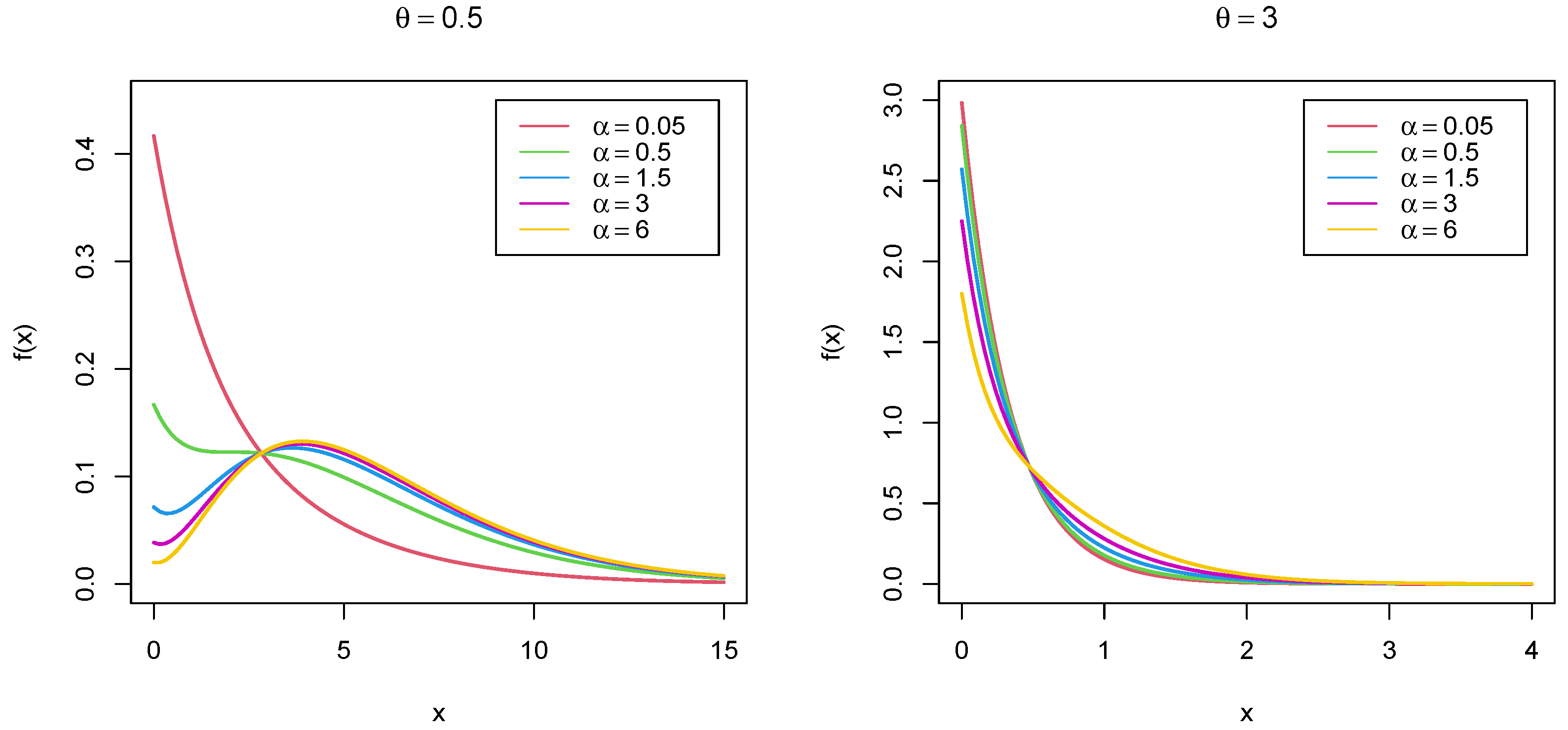
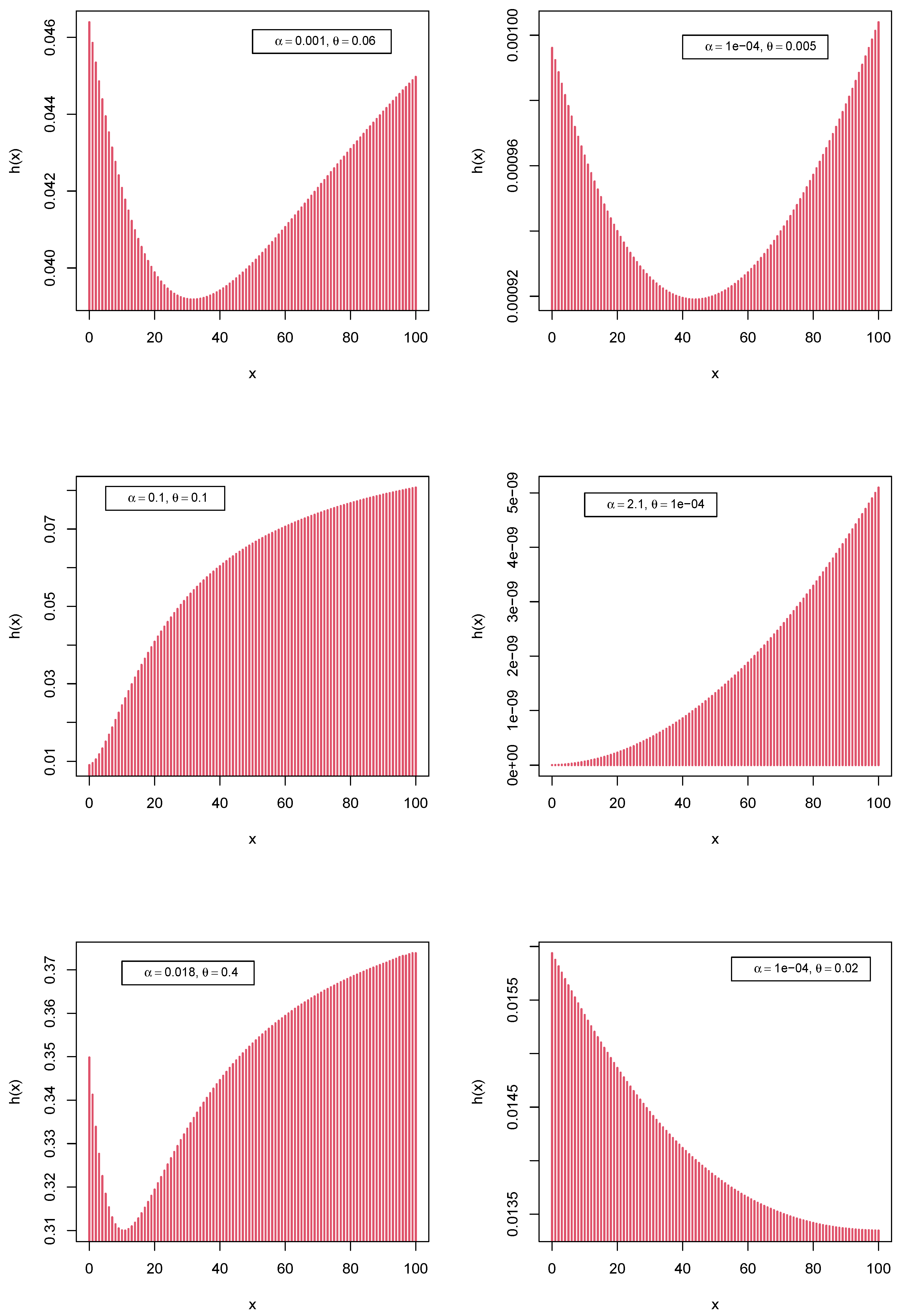
2. The Mirra Distribution
3. The Poisson–Mirra Distribution
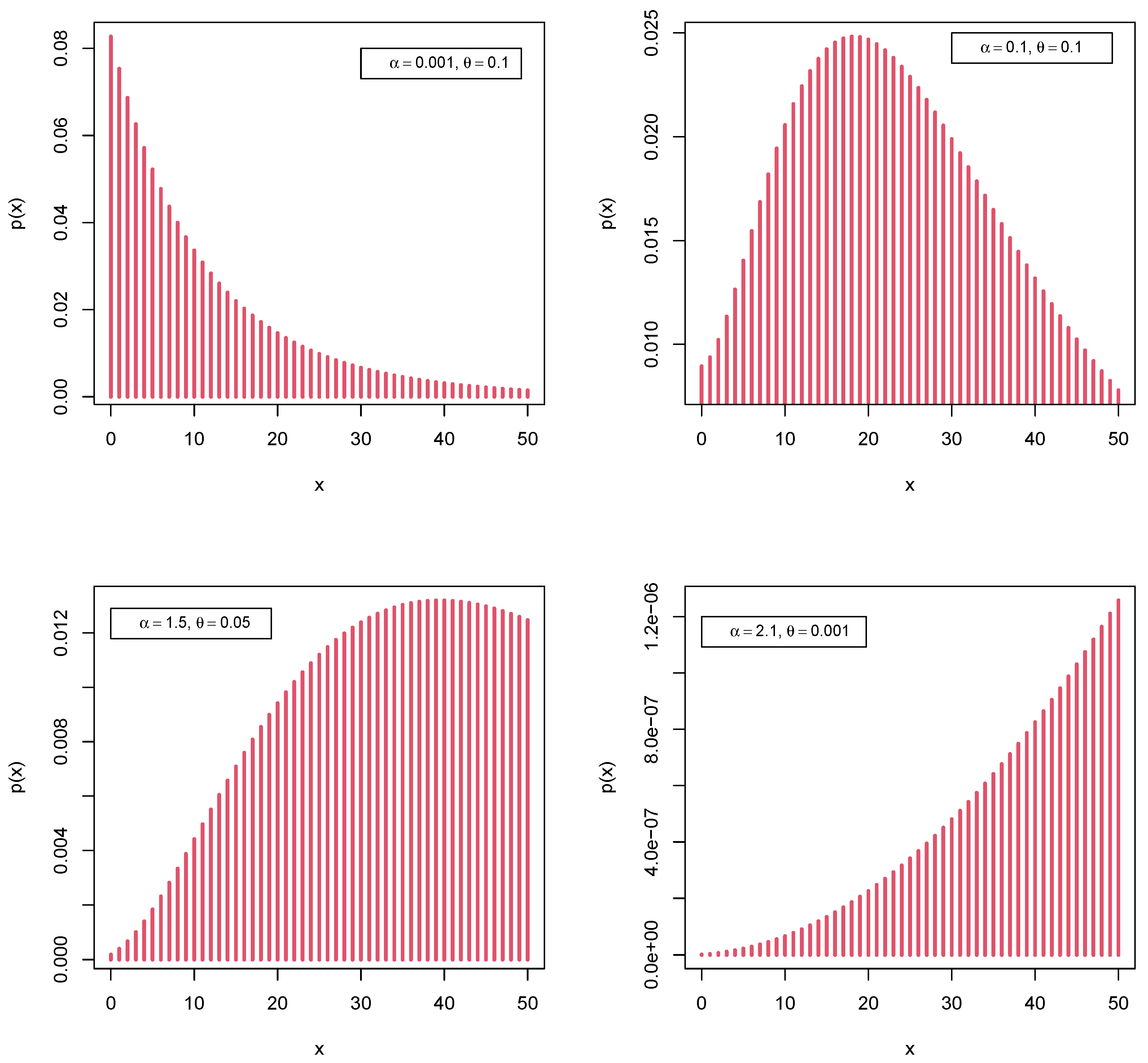
3.1. Presentation
3.2. Mode
3.3. Cdf and Hf
3.4. Moments
3.5. Rényi and Shannon Entropies
4. Estimation of the Parameters
4.1. Maximum Likelihood Estimation
4.2. Bayesian Estimation
4.3. Performance of the PMiD Parameters Using Simulation Study
5. PMiD Regression Model
6. INAR(1) Model with PMiD Innovations
7. Estimation of the Parameters: PMiD-INAR(1) Process
7.1. Conditional Maximum Likelihood (CML) Estimation
7.2. Conditional Least Squares (CLS) Estimation
7.3. Yule–Walker (YW) Estimation
7.4. Simulation: PMiD-INAR(1) Process
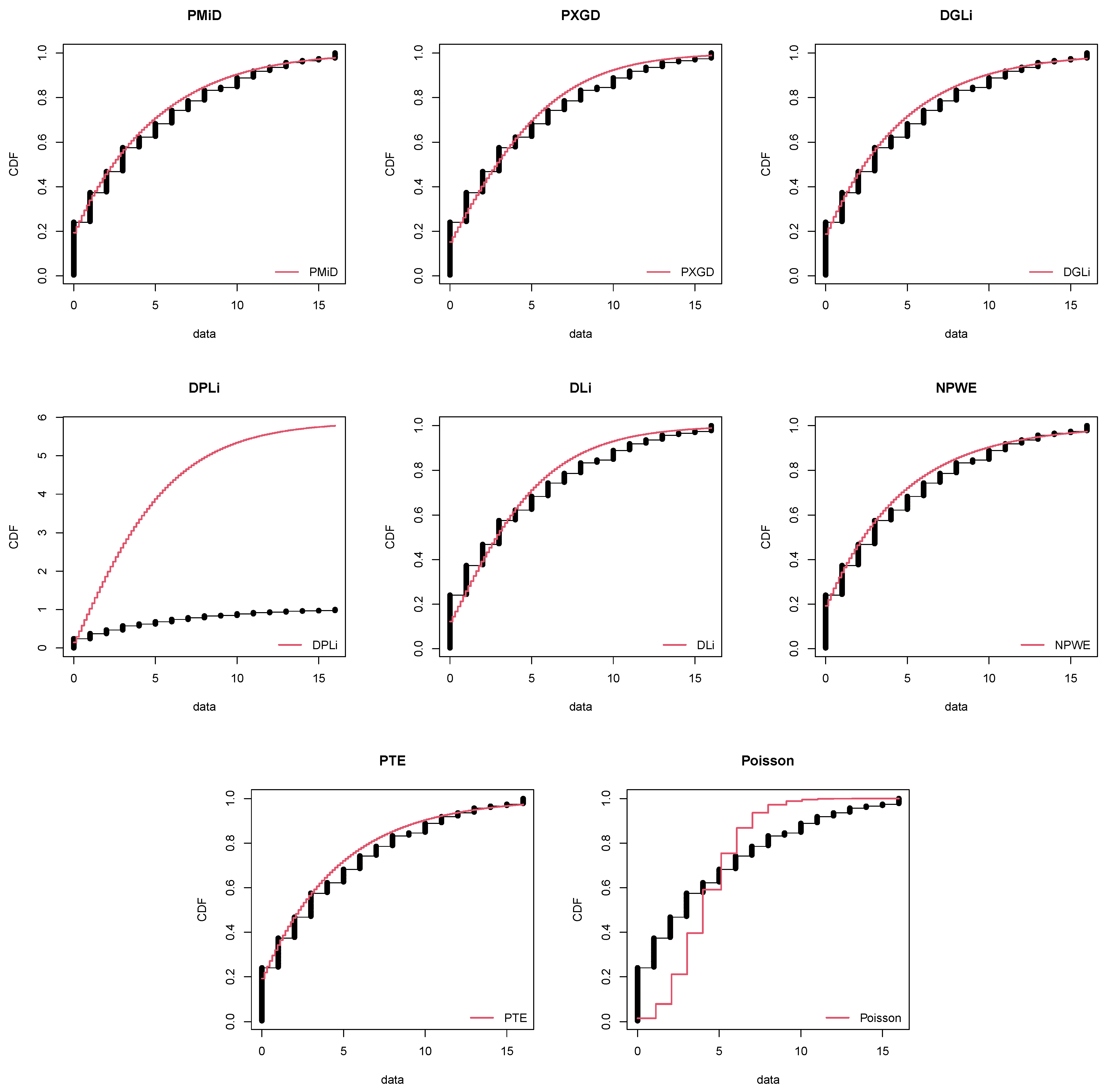
8. Applications and Empirical Study
8.1. COVID-19 Data: Armenia
8.2. Length of Hospital Stay
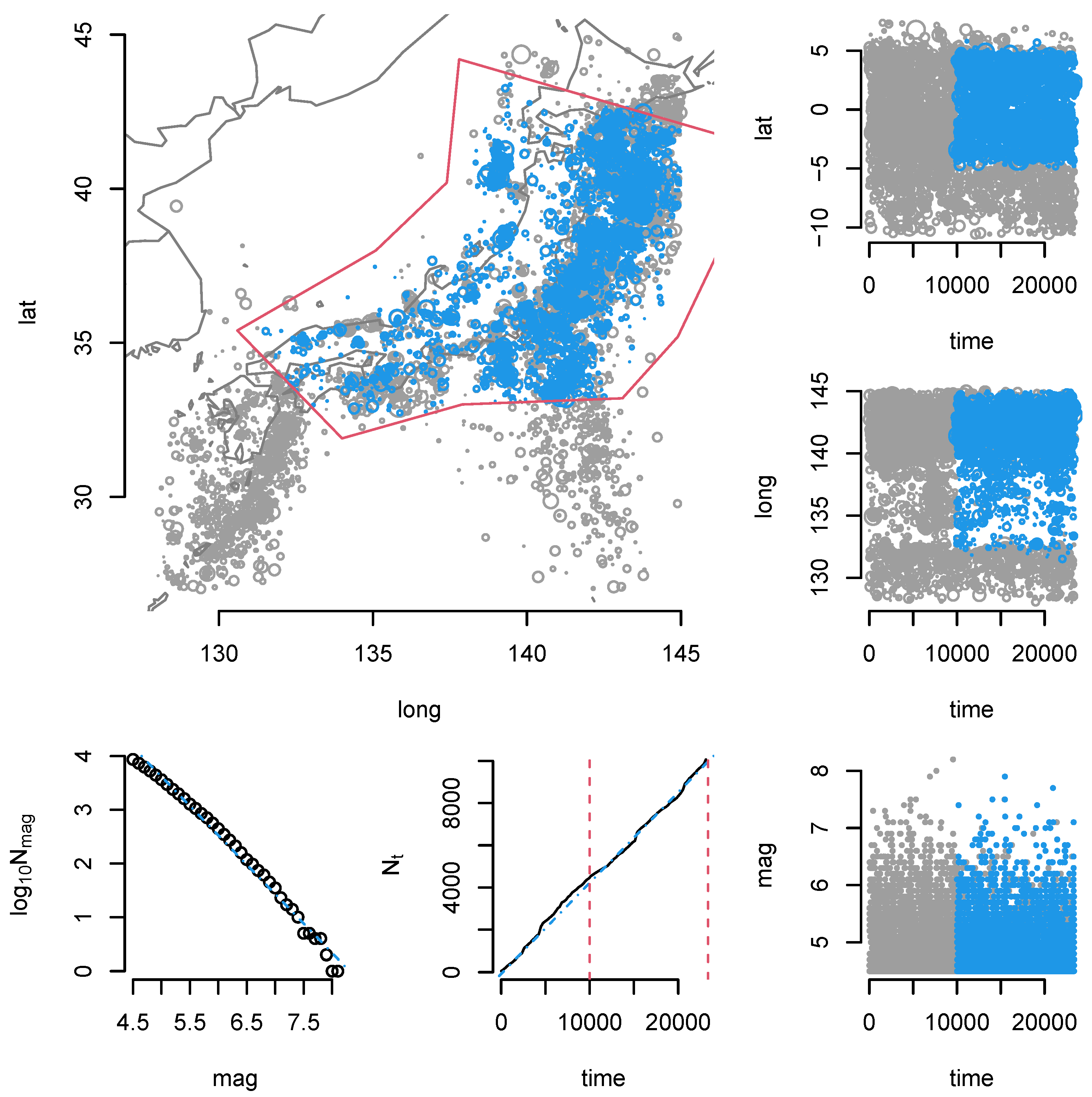
8.3. Japan Earthquake Data
9. Discussion
9.1. Context
9.2. This Work
9.3. Contributions and Limitations
9.4. Future Work
10. Conclusions
Author Contributions
Funding
Acknowledgments
Conflicts of Interest
Abbreviations
| INAR(1) | First-order Integer-valued Autoregressive |
| NB | Negative Binomial |
| PL | Poisson–Lindley |
| PMiD | Poisson–Mirra Distribution |
| MiD | Mirra Distribution |
| XGD | Xgamma Distribution |
| Probability Density Function | |
| cdf | Cumulative Distribution Function |
| sf | Survival Function |
| hf | Hazard Function |
| pmf | Probability Mass Function |
| PXGD | Poisson–Xgamma Distribution |
| DI | Dispersion Index |
| pgf | Probability Generating Function |
| mgf | Moment Generating Function |
| cf | Characteristic Function |
| MLE | Maximum Likelihood Estimate |
| hC | half-Cauchy |
| MHA | Metropolis–Hastings Algorithm |
| MCMC | Markov Chain Monte Carlo |
| MSE | Mean Squared Error |
| CP | Coverage Probability |
| AL | Average Length |
| CML | Conditional Maximum Likelihood |
| CLS | Conditional Least Squares |
| YW | Yule–Walker |
| ACF | Autocorrelation Function |
| MRE | Mean Relative Error |
| AIC | Akaike Information Criterion |
| BIC | Bayesian Information Criterion |
| GOF | Goodness-of-Fit |
| DGLi | Discrete Generalized Lindley |
| DPLi | Discrete Poisson–Lindley |
| DLi | Discrete Lindley |
| NPWE | New Poisson-Weighted Exponential |
| PTE | Poisson-Transmuted Exponential |
| SE | Standard Error |
| CI | Confidence Interval |
| df | Degrees of Freedom |
Appendix A
References
- Rigby, R.; Stasinopoulos, D.; Akantziliotou, C. A framework for modelling overdispersed count data, including the poisson-shifted generalized inverse gaussian distribution. Comput. Stat. Data Anal. 2008, 53, 381–393. [Google Scholar] [CrossRef]
- Sellers, K.F.; Raim, A. A flexible zero-inflated model to address data dispersion. Comput. Stat. Data Anal. 2016, 99, 68–80. [Google Scholar] [CrossRef]
- Contreras-Reyes, J.E. Lerch distribution based on maximum nonsymmetric entropy principle: Application to Conway’s game of life cellular automaton. Chaos Solitons Fractals 2021, 151, 111272. [Google Scholar] [CrossRef]
- Al-Osh, M.A.; Alzaid, A.A. First-order integer-valued autoregressive (INAR(1)) process. J. Time Ser. Anal. 1987, 8, 261–275. [Google Scholar] [CrossRef]
- McKenzie, E. Some simple models for discrete variate time series1. JAWRA J. Am. Water Resour. Assoc. 1985, 21, 645–650. [Google Scholar] [CrossRef]
- McKenzie, E. Autoregressive moving-average processes with negative-binomial and geometric marginal distributions. Adv. Appl. Probab. 1986, 18, 679–705. [Google Scholar] [CrossRef]
- Jung, R.; Ronning, G.; Tremayne, A. Estimation in conditional first order autoregression with discrete support. Stat. Pap. 2005, 46, 195–224. [Google Scholar] [CrossRef]
- Jazi, M.A.; Jones, G.; Lai, C.-D. Integer valued ar(1) with geometric innovations. J. Iran. Stat. Soc. 2012, 11, 173–190. [Google Scholar]
- Lívio, T.; Khan, N.M.; Bourguignon, M.; Bakouch, H. An inar(1) model with poisson-lindley innovations. Econ. Bull. 2018, 38, 1505–1513. [Google Scholar]
- Altun, E. A new one-parameter discrete distribution with associated regression and integer-valued autoregressive models. Math. Slovaca 2020, 70, 979–994. [Google Scholar] [CrossRef]
- Sen, S.; Ghosh, S.; Al-Mofleh, H. The Mirra distribution for modeling time-to-event data sets. In Strategic Management, Decision Theory, and Decision Science; Sinha, B.K., Bagchi, S.B., Eds.; Springer: Singapore, 2021; pp. 59–73. [Google Scholar]
- Sen, S.; Maiti, S.; Chandra, N. The xgamma distribution: Statistical properties and application. J. Mod. Appl. Stat. Methods 2016, 15, 774–788. [Google Scholar] [CrossRef] [Green Version]
- Altun, E.; Cordeiro, G.M.; Ristić, M.M. An one-parameter compounding discrete distribution. J. Appl. Stat. 2021, 1–22. [Google Scholar] [CrossRef]
- Sankaran, M. The discrete poisson-lindley distribution. Biometrics 1970, 26, 145–149. [Google Scholar] [CrossRef]
- R Core Team. R: A Language and Environment for Statistical Computing; R Foundation for Statistical Computing: Vienna, Austria, 2021; Available online: https://www.R-project.org/ (accessed on 6 September 2021).
- Gelman, A.; Hill, J. Data Analysis Using Regression and Multilevel/Hierarchical Models; Analytical Methods for Social Research; Cambridge University Press: Cambridge, UK, 2006. [Google Scholar]
- Weiß, C. An Introduction to Discrete-Valued Time Series; John Wiley & Sons, Ltd.: Hoboken, NJ, USA, 2018. [Google Scholar]
- Alzaid, A.; Alosh, M. First-order integer-valued autoregressive (inar (1)) process: Distributional and regression properties. Stat. Neerl. 1988, 42, 53–61. [Google Scholar] [CrossRef]
- El-morshedy, M.; Altun, E.; Eliwa, M.S. A new statistical approach to model the counts of novel coronavirus cases. Math. Sci. 2021, 1–14. [Google Scholar] [CrossRef]
- Gómez-Déniz, E.; Calderín-Ojeda, E. The discrete lindley distribution: Properties and applications. J. Stat. Comput. Simul. 2011, 81, 1405–1416. [Google Scholar] [CrossRef]
- Altun, E. A new generalization of geometric distribution with properties and applications. Commun. Stat.-Simul. Comput. 2020, 49, 793–807. [Google Scholar] [CrossRef]
- Bhati, D.; Kumawat, P.; Gómez-Déniz, E. A new count model generated from mixed poisson transmuted exponential family with an application to health care data. Commun. Stat. Theory Methods 2017, 46, 11060–11076. [Google Scholar] [CrossRef]
- Jalilian, A. Etas: An r package for fitting the space-time etas model to earthquake data. J. Stat. Software Code Snippets 2019, 88, 1–39. [Google Scholar] [CrossRef] [Green Version]


| and Various Values of | |||||
|---|---|---|---|---|---|
| Measures | |||||
| Mean | 0.9091 | 0.3081 | 0.1877 | 0.1357 | 0.1064 |
| Variance | 1.7796 | 0.4085 | 0.2240 | 0.1544 | 0.1179 |
| DI | 1.9576 | 1.3256 | 1.1931 | 1.1379 | 1.1076 |
| Skewness | 2.1407 | 2.5913 | 2.9319 | 3.2482 | 3.5398 |
| Kurtosis | 9.3872 | 11.8878 | 13.6830 | 15.5978 | 17.5592 |
| and Various Values of | |||||
| Measures | |||||
| Mean | 1.2 | 0.3481 | 0.1990 | 0.1403 | 0.1087 |
| Variance | 2.4267 | 0.4792 | 0.2411 | 0.1608 | 0.1209 |
| DI | 2.0222 | 1.3769 | 1.2117 | 1.1462 | 1.1118 |
| Skewness | 1.8289 | 2.5314 | 2.9032 | 3.2258 | 3.5212 |
| Kurtosis | 7.4713 | 11.5402 | 13.5972 | 15.5194 | 17.4747 |
| Parameters | n | MLE | Bias | MSE | CP | AL |
|---|---|---|---|---|---|---|
| 100 | 2.8296 | 0.3296 | 5.4612 | 0.8302 | 18.9348 | |
| 250 | 2.9959 | 0.4959 | 4.3959 | 0.8701 | 12.1873 | |
| 500 | 2.9402 | 0.4402 | 2.7254 | 0.9131 | 7.6664 | |
| 750 | 2.8896 | 0.3896 | 2.1199 | 0.9171 | 5.9141 | |
| 1000 | 2.8283 | 0.3283 | 1.5774 | 0.9181 | 4.8197 | |
| 100 | 0.4922 | −0.0078 | 0.0019 | 0.9570 | 0.1855 | |
| 250 | 0.4973 | −0.0027 | 0.00075 | 0.9630 | 0.1161 | |
| 500 | 0.4989 | −0.0011 | 0.00038 | 0.9640 | 0.0816 | |
| 750 | 0.4998 | −0.00023 | 0.00025 | 0.9710 | 0.0666 | |
| 1000 | 0.5003 | 0.00031 | 0.0002 | 0.9610 | 0.0578 |
| n | CML | CLS | YW | |||||||
|---|---|---|---|---|---|---|---|---|---|---|
| Bias | MSE | MRE | Bias | MSE | MRE | Bias | MSE | MRE | ||
| p | 100 | −0.0029 | 0.0021 | 0.9943 | 0.0366 | 0.0079 | 0.9269 | −0.0674 | 0.0181 | 0.8653 |
| 250 | −0.0017 | 0.00095 | 0.9966 | −0.0137 | 0.0030 | 0.9725 | −0.0246 | 0.0047 | 0.9508 | |
| 500 | −0.0015 | 0.00054 | 0.9984 | −0.0069 | 0.0016 | 0.9862 | −0.0101 | 0.0019 | 0.9799 | |
| 750 | −0.0012 | 0.00035 | 0.9966 | −0.0056 | 0.0011 | 0.9888 | −0.0070 | 0.0013 | 0.9859 | |
| 1000 | −0.0011 | 0.00029 | 0.9979 | −0.0027 | 0.0008 | 0.9946 | −0.0037 | 0.0008 | 0.9927 | |
| 100 | 0.0701 | 0.1251 | 1.1169 | 0.0826 | 0.0248 | 1.1377 | 1.8696 | 20.5181 | 4.1161 | |
| 250 | 0.0628 | 0.0957 | 1.1047 | 0.0517 | 0.0107 | 1.0862 | 0.9482 | 7.7421 | 2.5804 | |
| 500 | 0.0483 | 0.0740 | 1.0805 | 0.0456 | 0.0071 | 1.0760 | 0.4234 | 1.8246 | 1.7056 | |
| 750 | 0.0456 | 0.0617 | 1.0760 | 0.0427 | 0.0053 | 1.0712 | 0.2460 | 0.7204 | 1.4099 | |
| 1000 | 0.0421 | 0.0566 | 1.0785 | 0.0384 | 0.0044 | 1.0641 | 0.1495 | 0.2579 | 1.2492 | |
| 100 | −0.0203 | 0.0120 | 0.9710 | −0.0151 | 0.0049 | 0.9784 | 0.0291 | 0.1533 | 1.0416 | |
| 250 | −0.0092 | 0.0058 | 0.9868 | −0.0016 | 0.0020 | 0.9979 | −0.0083 | 0.0236 | 0.9881 | |
| 500 | −0.0057 | 0.0038 | 0.9918 | 0.0014 | 0.0011 | 1.0022 | −0.0047 | 0.0091 | 0.9933 | |
| 750 | −0.0032 | 0.0021 | 0.9954 | 0.0011 | 0.0008 | 1.0038 | −0.0040 | 0.0044 | 0.9943 | |
| 1000 | −0.0011 | 0.0018 | 0.9984 | 0.0009 | 0.0006 | 1.0067 | −0.0021 | 0.0035 | 0.9970 | |
| Distribution | Abbreviation | Reference |
|---|---|---|
| Discrete generalized Lindley | DGLi | [19] |
| Poisson–Xgamma | PXGD | [13] |
| Discrete Poisson–Lindley | DPLi | [9] |
| Discrete Lindley | DLi | [20] |
| New Poisson-weighted exponential | NPWE | [21] |
| Poisson-transmuted exponential | PTE | [22] |
| Poisson | P | - |
| Distribution | ||||||
|---|---|---|---|---|---|---|
| MLE | SE | CI | MLE | SE | CI | |
| PMiD | 0.1029 | 0.0586 | (−0.0121, 0.2178) | 0.4162 | 0.0463 | (0.3254, 0.5070) |
| PXGD | 0.5431 | 0.0275 | (0.4892, 0.5969) | - | - | - |
| DGLi | 0.2477 | 0.0843 | (0.0825, 0.4128) | 0.7763 | 0.0316 | (0.7144, 0.8382) |
| DPLi | 0.41001 | 0.0227 | (0.3656, 0.4545) | - | - | - |
| DLi | 0.6914 | 0.0121 | (0.6677, 0.7151) | - | - | - |
| NPWE | 0.2167 | 3.1158 | (−5.8903, 6.3236) | 0.1008 | 15.8322 | (−30.9297, 31.1313) |
| PTE | 0.0001 | 0.2144 | (−0.4202, 0.4202) | 0.2385 | 0.0303 | (0.1790, 0.2980) |
| P | 4.1931 | 0.1342 | (−3.9302, 4.4561) | - | - | - |
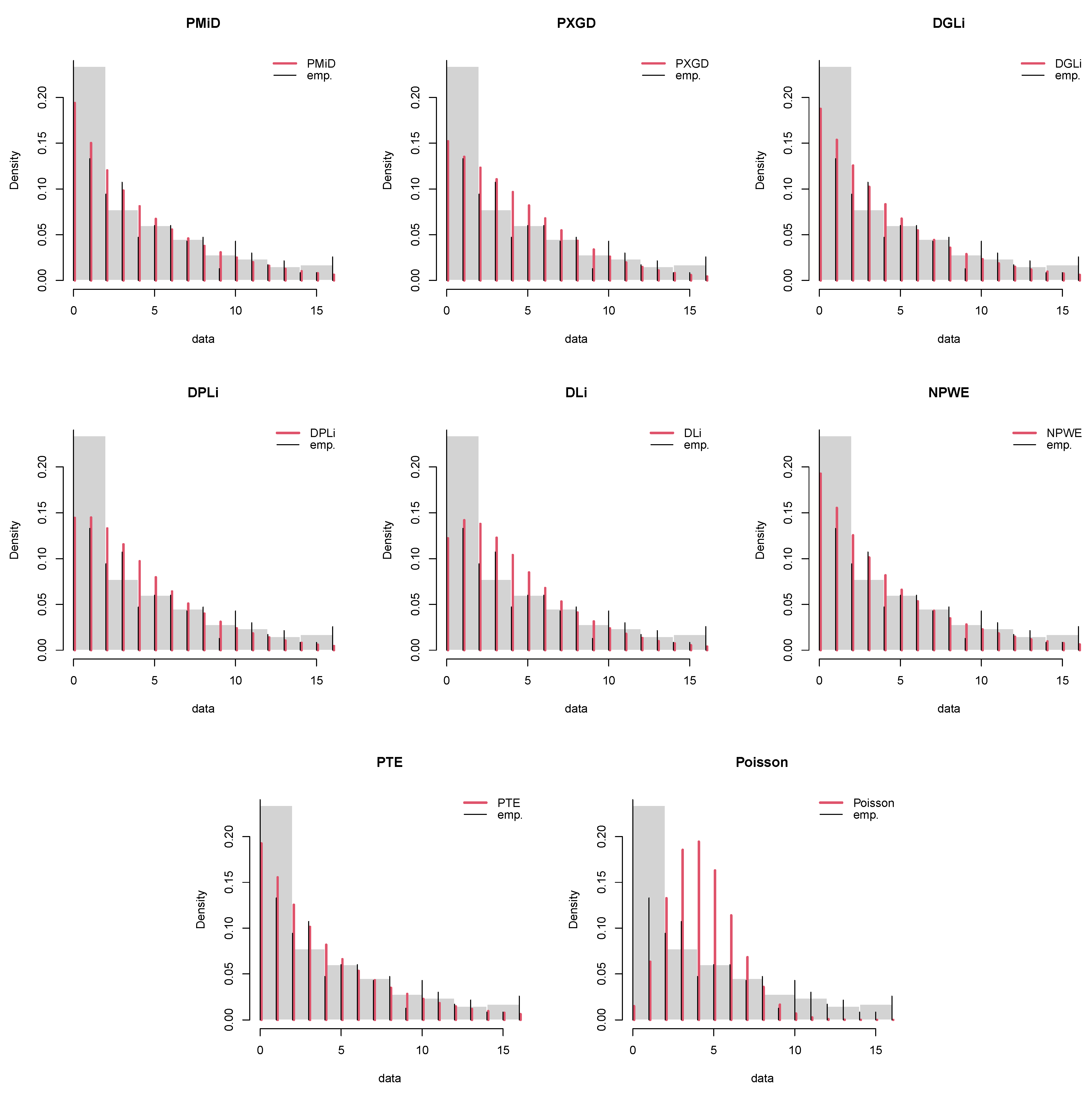
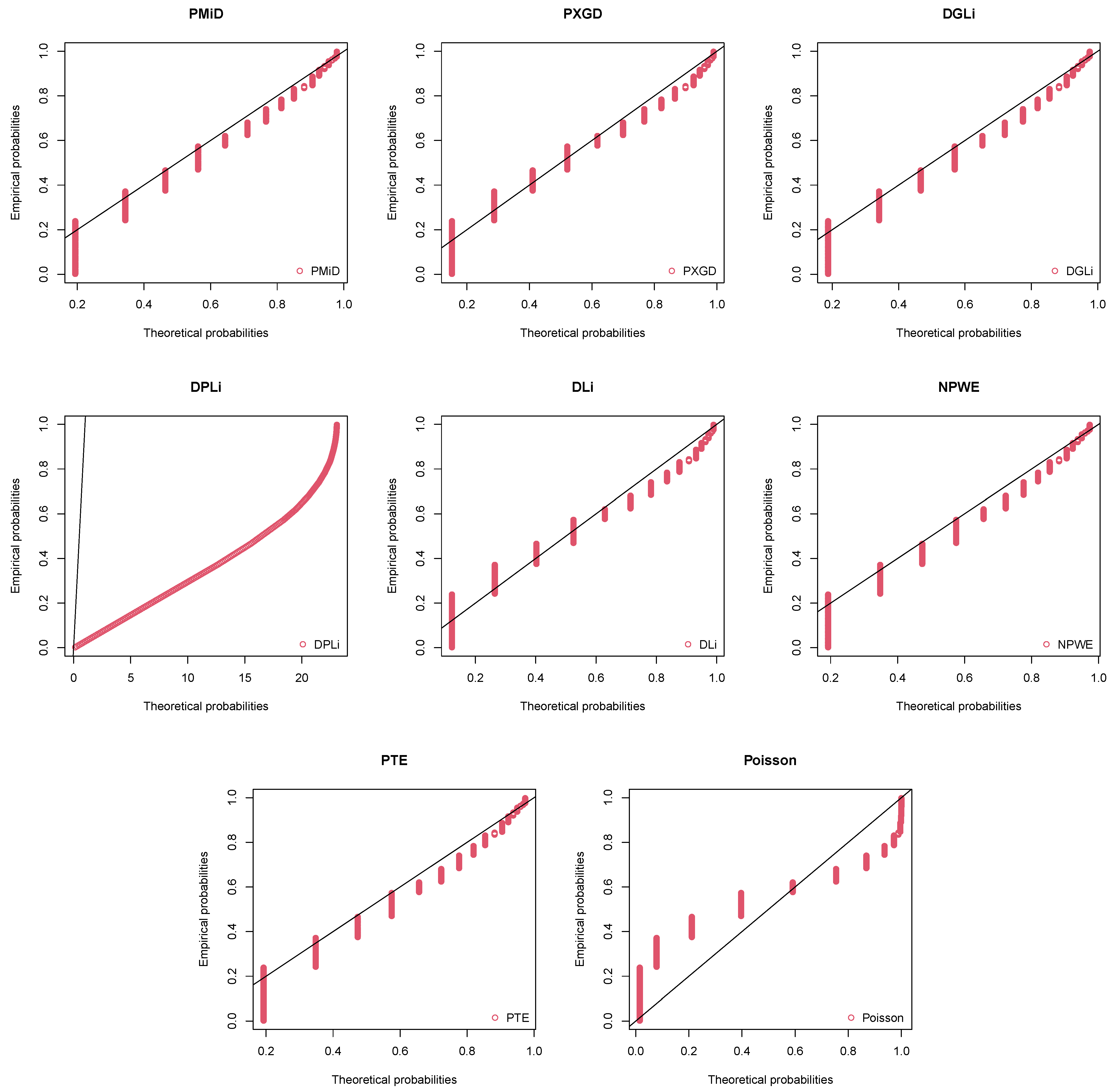
| X | OF | Expected Frequency | |||||||
|---|---|---|---|---|---|---|---|---|---|
| PMiD | PXGD | DGLi | DPLi | DLi | NPWE | PTE | P | ||
| 0 | 56 | 45.1654 | 35.4419 | 43.6875 | 33.6739 | 28.4819 | 44.8674 | 44.8672 | 3.5181 |
| 1 | 31 | 35.0039 | 31.4999 | 35.8015 | 33.7917 | 33.0940 | 36.2276 | 36.2274 | 14.7516 |
| 2 | 22 | 28.0128 | 28.7071 | 29.2575 | 30.9936 | 32.1465 | 29.2515 | 29.2514 | 30.9278 |
| 3 | 25 | 22.8835 | 25.7701 | 23.8497 | 26.9655 | 28.6318 | 23.6187 | 23.6186 | 43.2281 |
| 4 | 11 | 18.8974 | 22.5056 | 19.3972 | 22.6594 | 24.2248 | 19.0706 | 19.0705 | 45.3153 |
| 5 | 14 | 15.6646 | 19.0995 | 15.7433 | 18.5775 | 19.8108 | 15.3983 | 15.3982 | 38.0026 |
| 6 | 14 | 12.9730 | 15.7909 | 12.7535 | 14.9535 | 15.8141 | 12.4331 | 12.4331 | 26.5583 |
| 7 | 10 | 10.7033 | 12.7614 | 10.3135 | 11.8663 | 12.3974 | 10.0389 | 10.0390 | 15.9089 |
| 8 | 11 | 8.7834 | 10.1133 | 8.3269 | 9.3101 | 9.5833 | 8.1058 | 8.1059 | 8.3385 |
| 9 | 3 | 7.1637 | 7.8812 | 6.7131 | 7.2372 | 7.3255 | 6.5449 | 6.5450 | 3.8850 |
| 10 | 10 | 5.8053 | 6.0535 | 5.4045 | 5.5826 | 5.5485 | 5.2846 | 5.2846 | 1.6290 |
| 11 | 7 | 4.6746 | 4.5919 | 4.3455 | 4.2783 | 4.1706 | 4.2670 | 4.2670 | 0.6210 |
| 12 | 4 | 3.7409 | 3.4454 | 3.4898 | 3.2605 | 3.1147 | 3.4453 | 3.4453 | 0.2170 |
| 13 | 5 | 2.9762 | 2.5607 | 2.7995 | 2.4729 | 2.3133 | 2.7819 | 2.7818 | 0.0700 |
| 14 | 2 | 2.3547 | 1.8870 | 2.2434 | 1.8676 | 1.7099 | 2.2462 | 2.2462 | 0.0210 |
| 15 | 2 | 1.8534 | 1.3802 | 1.7960 | 1.4053 | 1.2586 | 1.8136 | 1.8140 | 0.0059 |
| ≥16 | 6 | 6.3439 | 3.5106 | 7.0775 | 4.1044 | 3.3744 | 7.6048 | 7.6049 | 0.0020 |
| Total | 233 | 233 | 233 | 233 | 233 | 233 | 233 | 233 | |
| 590.3751 | 596.7075 | 592.6174 | 598.9318 | 605.3913 | 592.7991 | 592.7991 | 827.4472 | ||
| AIC | 1184.750 | 1195.415 | 1189.235 | 1199.864 | 1212.783 | 1189.598 | 1189.598 | 1656.894 | |
| BIC | 1191.652 | 1198.866 | 1196.137 | 1203.315 | 1216.234 | 1196.500 | 1196.500 | 1660.345 | |
| 9.3187 | 25.1615 | 12.3710 | 28.1328 | 45.7236 | 12.0550 | 12.0549 | 483.1912 | ||
| df | 6 | 7 | 6 | 8 | 7 | 6 | 6 | 7 | |
| p value | 0.1564 | <0.001 | 0.0542 | 0.0004 | <0.001 | 0.0608 | 0.0607 | <0.001 | |
| Parameter | ML | Bayes |
|---|---|---|
| 0.1029 | 0.1688 | |
| 0.4162 | 0.4515 |
| Covariates | Poisson | NPWE | PXGD | PMiD | ||||
|---|---|---|---|---|---|---|---|---|
| Estimate (SE) | p-Value | Estimate (SE) | p-Value | Estimate (SE) | p-Value | Estimate (SE) | p-Value | |
| 1.4560 (0.0159) | <0.001 | 1.3871 (0.0458) | <0.001 | 1.3996 (0.0349) | <0.001 | 2.1007 (0.0228) | <0.001 | |
| 0.9604 (0.0122) | <0.001 | 0.9982 (0.0363) | <0.001 | 0.9721 (0.0270) | <0.001 | 0.3693 (0.0789) | <0.001 | |
| −0.1240 (0.0118) | <0.001 | −0.1276 (0.0380) | <0.001 | −0.1269 (0.0280) | <0.001 | −0.0553 (0.0130) | <0.001 | |
| 0.3266 (0.0121) | <0.001 | 0.4047 (0.0376) | <0.001 | 0.1201 (0.0298) | <0.001 | 0.2087 (0.0220) | <0.001 | |
| 0.1222 (0.0125) | <0.001 | 0.1189 (0.0405) | <0.001 | 0.3732 (0.0280) | <0.001 | 0.0309 (0.0108) | <0.001 | |
| − | 0.5311 (1.4829 × 10³) | 0.9997 | − | 0.3296 (0.0054) | <0.001 | |||
| L | 11,189.90 | 11,194.01 | 10,569.80 | 10,382.38 | ||||
| AIC | 22,389.80 | 22,400.02 | 21,149.60 | 20,776.76 | ||||
| BIC | 22,420.72 | 22,437.13 | 21,180.60 | 20,813.88 | ||||
| Model | Parameters | Estimate | SE | L | AIC | BIC |
|---|---|---|---|---|---|---|
| INAR-PMiD(1) | p | 0.2813 | 0.0293 | 446.0982 | 898.1965 | 905.4166 |
| 0.6869 | 2.8522 | |||||
| 0.0247 | 0.0019 | |||||
| INAR-NPWE(1) | p | 0.3503 | 0.0204 | 465.8715 | 937.7431 | 944.9632 |
| 0.0068 | 0.0043 | |||||
| 0.3408 | 0.8622 | |||||
| INAR-PTE(1) | p | 0.0320 | 0.0293 | 451.1948 | 908.3896 | 915.6098 |
| −0.9999 | 0.2543 | |||||
| 0.0130 | 0.00124 | |||||
| INAR-DPLi(1) | p | 0.3179 | 0.0238 | 450.902 | 905.804 | 910.6174 |
| 0.0172 | 0.0015 | |||||
| PINAR(1) | p | 0.0592 | 0.0145 | 1418.918 | 2841.836 | 2846.65 |
| 158.6002 | 2.7801 |
Publisher’s Note: MDPI stays neutral with regard to jurisdictional claims in published maps and institutional affiliations. |
© 2022 by the authors. Licensee MDPI, Basel, Switzerland. This article is an open access article distributed under the terms and conditions of the Creative Commons Attribution (CC BY) license (https://creativecommons.org/licenses/by/4.0/).
Share and Cite
Maya, R.; Irshad, M.R.; Chesneau, C.; Nitin, S.L.; Shibu, D.S. On Discrete Poisson–Mirra Distribution: Regression, INAR(1) Process and Applications. Axioms 2022, 11, 193. https://doi.org/10.3390/axioms11050193
Maya R, Irshad MR, Chesneau C, Nitin SL, Shibu DS. On Discrete Poisson–Mirra Distribution: Regression, INAR(1) Process and Applications. Axioms. 2022; 11(5):193. https://doi.org/10.3390/axioms11050193
Chicago/Turabian StyleMaya, Radhakumari, Muhammed Rasheed Irshad, Christophe Chesneau, Soman Latha Nitin, and Damodaran Santhamani Shibu. 2022. "On Discrete Poisson–Mirra Distribution: Regression, INAR(1) Process and Applications" Axioms 11, no. 5: 193. https://doi.org/10.3390/axioms11050193
APA StyleMaya, R., Irshad, M. R., Chesneau, C., Nitin, S. L., & Shibu, D. S. (2022). On Discrete Poisson–Mirra Distribution: Regression, INAR(1) Process and Applications. Axioms, 11(5), 193. https://doi.org/10.3390/axioms11050193