Article

Fractional Modelling and Optimal Control of COVID-19 Transmission in Portugal

by
Silvério Rosa
1,† and
Delfim F. M. Torres
2,*,†
1
Department of Mathematics, Instituto de Telecomunicações (IT), Universidade da Beira Interior, 6201-001 Covilhã, Portugal
2
Center for Research and Development in Mathematics and Applications (CIDMA), Department of Mathematics, University of Aveiro, 3810-193 Aveiro, Portugal
*
Author to whom correspondence should be addressed.
These authors contributed equally to this work.
Axioms 2022, 11(4), 170; https://doi.org/10.3390/axioms11040170
Submission received: 31 October 2021 / Revised: 25 March 2022 / Accepted: 6 April 2022 / Published: 11 April 2022
(This article belongs to the Special Issue Mathematics of the COVID-19)

Abstract

:
A fractional-order compartmental model was recently used to describe real data of the first wave of the COVID-19 pandemic in Portugal [Chaos Solitons Fractals 144 (2021), Art. 110652]. Here, we modify that model in order to correct time dimensions and use it to investigate the third wave of COVID-19 that occurred in Portugal from December 2020 to February 2021, and that has surpassed all previous waves, both in number and consequences. A new fractional optimal control problem is then formulated and solved, with vaccination and preventive measures as controls. A cost-effectiveness analysis is carried out, and the obtained results are discussed.

1. Introduction

In January 2020, the World Health Organization (WHO) announced the existence of a significant number of pneumonia cases in Wuhan. Against all the predictions, COVID-19 (COrona VIrus Disease-19) spread quickly across the globe and, on 11th of March, was declared as a pandemic [1]. Caused by SARS-CoV-2 (Severe Acute Respiratory Syndrome Corona Virus 2), COVID-19 is the first pandemic in the digital era from which very few territories of the world are untouched. Many governments were forced to decree measures that seemed to be outdated, such as the isolation of individuals and the complete lockdown of regions and even countries, that compromise individual freedoms, damage business and economy, and threaten a significant number of jobs.
To fight COVID-19 and its harmful effects, a multidisciplinary approach is needed. In particular, mathematical modelling plays an important role in the prediction of possible scenarios and in its effective control [2,3]. Readers interested in fractional modelling are referred to [4,5] and references therein.
The pandemic numbers have put national health systems under pressure. Many reported cases were not reported on time, but with a delay of days. Hence, in this paper, we do not use the number of daily reported cases but the means of the previous five days of reported cases, as suggested in [6].
The mean of five days of daily reported cases induces memory into the model. Fractional derivatives have been intensively used to obtain models of infectious diseases that take into account the memory effects. Many researchers have focused particular attention in modelling real-world phenomena using non-integer order derivatives. Those dynamics have been modelled and studied by using the concept of fractional-order derivatives. These problems appear in a range of diversified fields of applied sciences, including biology, physics, ecology, and engineering [7,8].
A classical compartmental model with a super-spreader class was firstly applied to give an estimation of infected subjects and fatalities in Wuhan, China, in [9]. The first-order derivative was then substituted by a derivative of a fractional order, resulting in a model investigated with Caputo fractional derivatives [6]. Here, this fractional model is corrected and then used to model the third wave of COVID-19 in Portugal. We start by the estimation of parameters that best fit the real data. The sensitivity analysis to the fractional-order model is performed in order to identify which model parameters are most influential on the dynamics of the disease. Afterwards, fractional optimal control is applied, showing the effectiveness of our approach.
This paper is organized as follows. In Section 2, the fractional order model is formulated. Our main results are then given in Section 3: parameter estimation of the COVID-19 model with real data of Portugal (Section 3.1); sensitivity analysis of the parameters of the model, without forgetting the effect of the order of fractional differentiation (Section 3.2); fractional optimal control of the model (Section 3.3); and, finally, numerical simulations and cost-effectiveness of the fractional model (Section 3.4). We end with Section 4, which states the conclusions. Our main theoretical contributions consist of fractional-order model consistency and the mathematical problem rearrangement according to the Pontryagin theory. Moreover, we solve the fractional optimal control problem numerically by a method of Adams–Basforth–Moulton.

2. Fractional-Order COVID-19 Model

Since the time interval considered in this study is small, we assume that population is invariant. In addition, population is divided in eight classes: (i) susceptible individuals, S; (ii) exposed individuals, E; (iii) symptomatic infectious individuals, I; (iv) super-spreader individuals, P; (v) asymptomatic infectious individuals, A; (vi) hospitalized individuals, H; (vii) recovered individuals, R; and (viii) fatality class, F. Our fractional-order model is derived from the one presented in Ndaïrou et al. [6], which gives a generalization of an integer-order model that was used to study the start of the pandemic in Wuhan [9]. We use the fractional derivative in the sense of Caputo. Fractional differential equations are an active area of research and are adequate to incorporate the history of the processes. The model system of equations for COVID-19 proposed in [6] is given by
0 C D t α S = β I S N l β H S N β P S N , 0 C D t α E = β I S N + l β H S N + β P S N κ E , 0 C D t α I = κ ρ 1 E ( γ a + γ i ) I δ i I , 0 C D t α P = κ ρ 2 E ( γ a + γ i ) P δ p P , 0 C D t α A = κ ( 1 ρ 1 ρ 2 ) E , 0 C D t α H = γ a ( I + P ) γ r H δ h H , 0 C D t α R = γ i ( I + P ) + γ r H , 0 C D t α F = δ i I + δ p P + δ h H ,
where 0 C D t α denotes the left Caputo fractional-order derivative with derivative order α ( 0 < α 1 ). A description of the parameters of Model (1) can be found in Table 1.
We note that the equations of Model (1) do not have appropriate time dimensions. Indeed, on the left-hand side, dimension is (time) α , while on the right-hand side, dimension is (time) 1 . This means that Model (1) is only consistent when α = 1 . For the importance to be consistent with dimensions, we refer the reader, e.g., to [11,12]. Thus, here, we correct System (1) as follows:
0 C D t α S = β α I S N l β α H S N β α P S N , 0 C D t α E = β α I S N + l β α H S N + β α P S N κ α E , 0 C D t α I = κ α ρ 1 E ( γ a α + γ i α ) I δ i α I , 0 C D t α P = κ α ρ 2 E ( γ a α + γ i α ) P δ p α P , 0 C D t α A = κ α ( 1 ρ 1 ρ 2 ) E , 0 C D t α H = γ a α ( I + P ) γ r α H δ h α H , 0 C D t α R = γ i α ( I + P ) + γ r α H , 0 C D t α F = δ i α I + δ p α P + δ h α H .
A flow diagram of Model (2) is given in Figure 1. Note that, in the particular case α = 1 , both Models (1) and (2) coincide with the classical COVID-19 model first introduced in [9]. System (2) will be investigated in Section 3.

3. Main Results

We begin by discussing the adherence of the corrected Model (2) introduced in Section 2 with respect to COVID-19 and real data from the third wave that occurred in Portugal. For that, we need an adequate estimation of the parameter values.

3.1. Parameter Estimation

The uncorrected model (1) was used to study the dynamics of COVID-19 at the early stage of the pandemic, between 3 March 2020 and 27 April 2020, in [6]. During that period, government decreed a general lockdown of the country that was well accepted by the population due to the impact of the disease in other countries where it started earlier. With limited knowledge, this revealed to be an effective measure to reduce contacts and control the disease in a relatively short period of time.
That initial stage ended in May 2020, with the gradual release of the country from COVID-19 container measures and the cancelling of the State of Emergency. In that date, preventive measures were adopted to control the disease. One of the most important was the use of masks in confined spaces, made mandatory by Portuguese Decreto-Lei n.º 20/2020.
In October 2020, due to autumn weather conditions, the number of infected individuals started to be worrisome. In order to control it and to protect the Portuguese National Health Service, in November 2020, a new series of States of Emergency began. In January 2021, the cold weather, some relaxation among the population concerning preventive measures (being in crowds or poorly ventilated spaces, the misuse of masks, …) combined with new variants of COVID-19—more contagious than ever— that started circulating, forced the government to declare a new lockdown with the closure of schools in 22 January 2021.
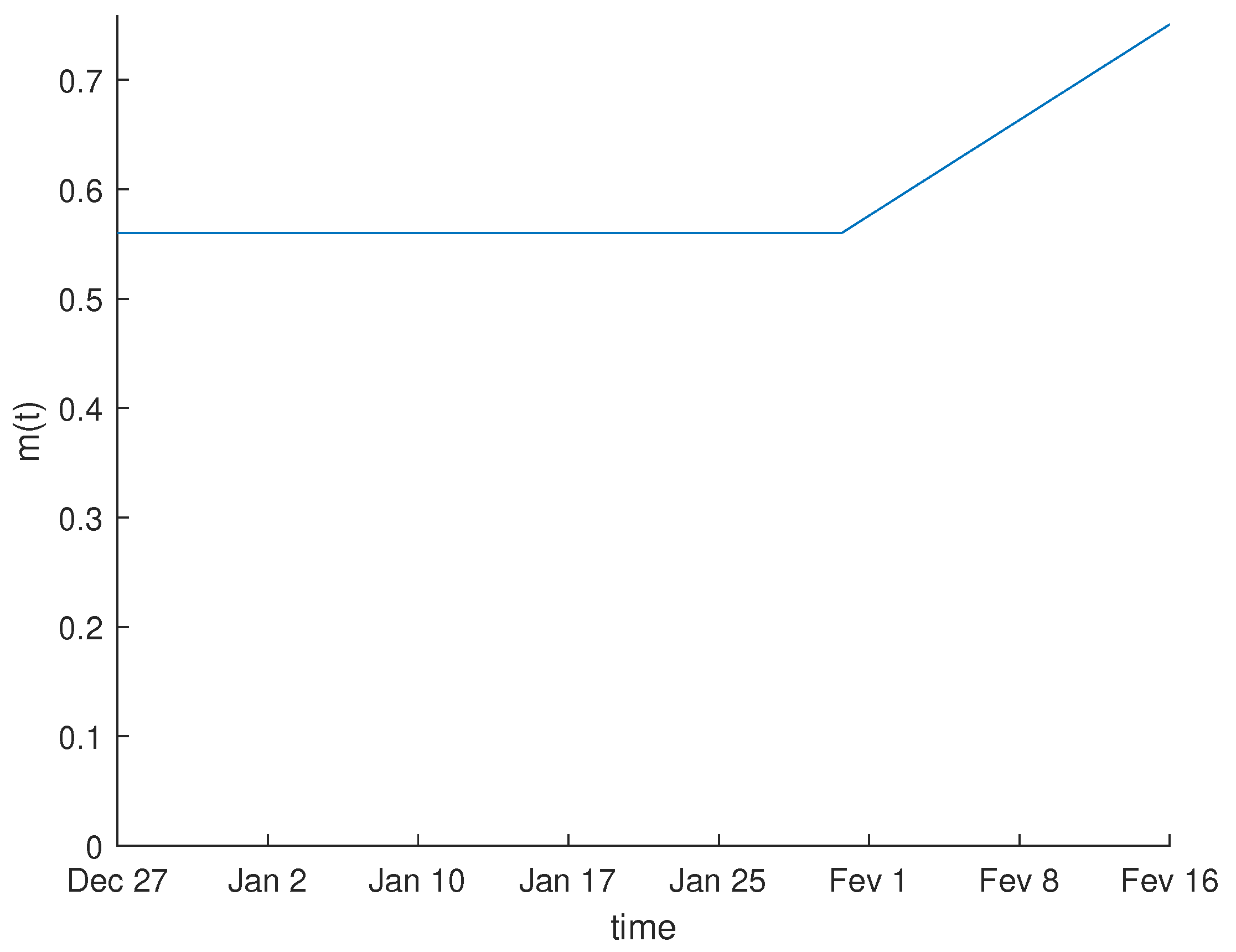
Due to the implementation of the preventive measures, during our model fitting, we assume that parameters have the same values of the first wave, with the exception of contact rates. The period we chose starts in 27 December 2020 and ends 16 February 2021, covering the third wave of the pandemic in Portugal. During that period, the closure of schools was declared, and that most certainly had an impact on contact rates. Hence, we consider that the transmission coefficient β is replaced by β ( 1 m ( t ) ) , and that β is replaced by β ( 1 m ( t ) ) , where m ( t ) is a continuous function that represents the rate of reduction of the contacts, and that varies with time according to Figure 2.
The values of two parameters were determined by the fitting of the model: (i) derivative order of the model, α , and (ii) a scaling factor s. See Table 2 for the resulting values and errors associated with the fitting.
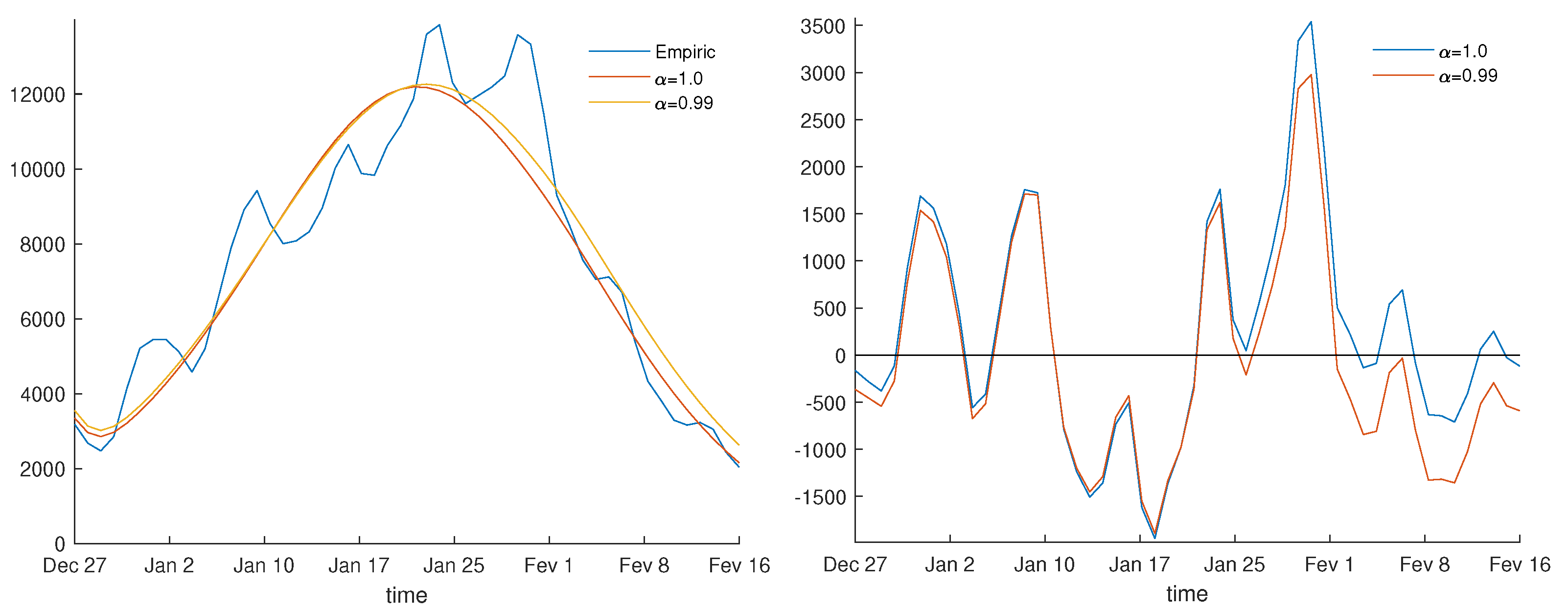
The fitting curves are presented in Figure 3, where real data was obtained from [13,14].
It is known that the available data has some mistakes. Frequently, days reporting few cases are followed by days reporting many new cases, without correspondence with reality. Due to the stress that the pandemic imposed over doctors and health professionals, these data do not flow as quickly and effectively as expected. Therefore, the numbers of new cases are not correctly determined by reported daily numbers. Thus, the number of new cases considered in this manuscript is, as suggested in [6], the mean of the previous five days of reported cases.
Following [15], our data fitting consisted in minimization of the l 2 norm of the difference between the real values and predictive cases of COVID-19 infection given by Model (2). Due to the oscillation of the number of confirmed cases per day, the fitting curves observed in Figure 3 (left) have significant gaps in comparison with real data. Figure 3 (right) presents the difference between the number of confirmed cases per day and the number of estimated cases, showing that the proposed model approximates well the average number of cases.
Consequently, fitting errors are quite high, being 14.13% for the classical integer-order model ( α = 1 ) and 13.37% for the fractional-order model with α = 0.99 , according to Table 2. The difference between the two derivative orders, in terms of absolute errors, justifies the preference for the fractional-order model with respect to the classical one.

3.2. Sensitivity Analysis

An important threshold, while studying infectious disease models, is the basic reproduction number. Following [9,10], we conclude that the basic reproduction number of the COVID-19 model (2) is
R 0 = β α ρ 1 ( γ a α l + a h ) a i a h + ( β α γ a α l + β α a h ) ρ 2 a p a h ,
where a i = γ a α + γ i α + δ i α , a p = γ a α + γ i α + δ p α and a h = γ r α + δ h α .
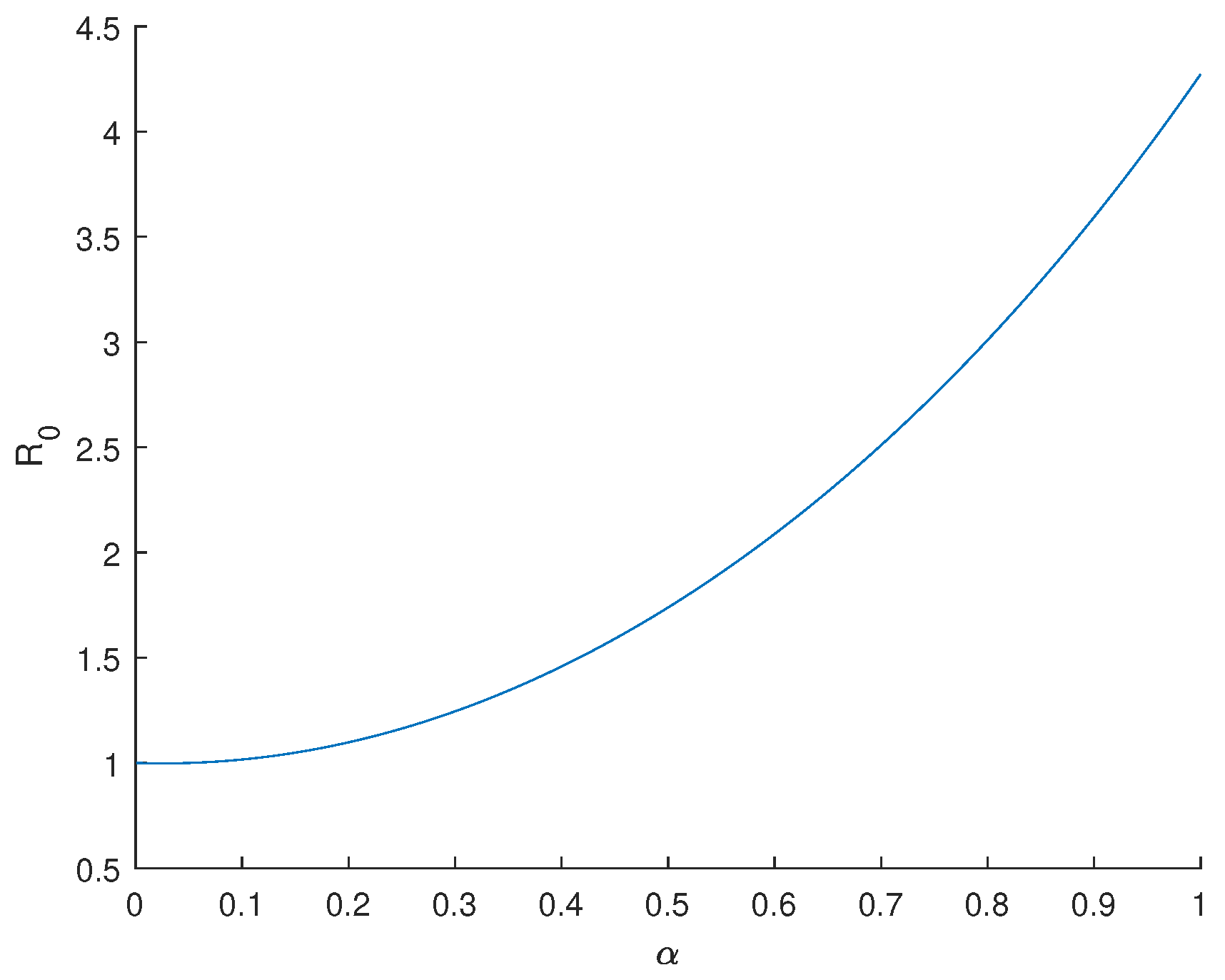
The impact of the variation of the derivative order α , in the evolution of R 0 , is presented in Figure 4. We observe in Figure 4 that R 0 1 , that is, we have an endemic scenario regardless of the value of α .
Sensitivity analysis measures the importance of each parameter of the model in the disease transmission.
Definition 1
(The sensitivity index [16,17]). Let R 0 be differentiable with respect to a given parameter p. The sensitivity of the model with respect to that parameter p can be measured by the index Υ p R 0 given by
Υ p R 0 = R 0 p p R 0 .
The sensitivity analysis of the classical COVID-19 model was presented in [9], that is, in the particular situation α = 1 in (2). In it, the authors concluded that the most sensitive parameters to the basic reproduction number R 0 are β , ρ 1 , and l. Therefore, special attention should be paid to the estimation of those parameters. In contrast, the estimation of β , ρ 2 , γ a , δ i , δ p , and δ h does not require as much attention because of its low sensitivity.
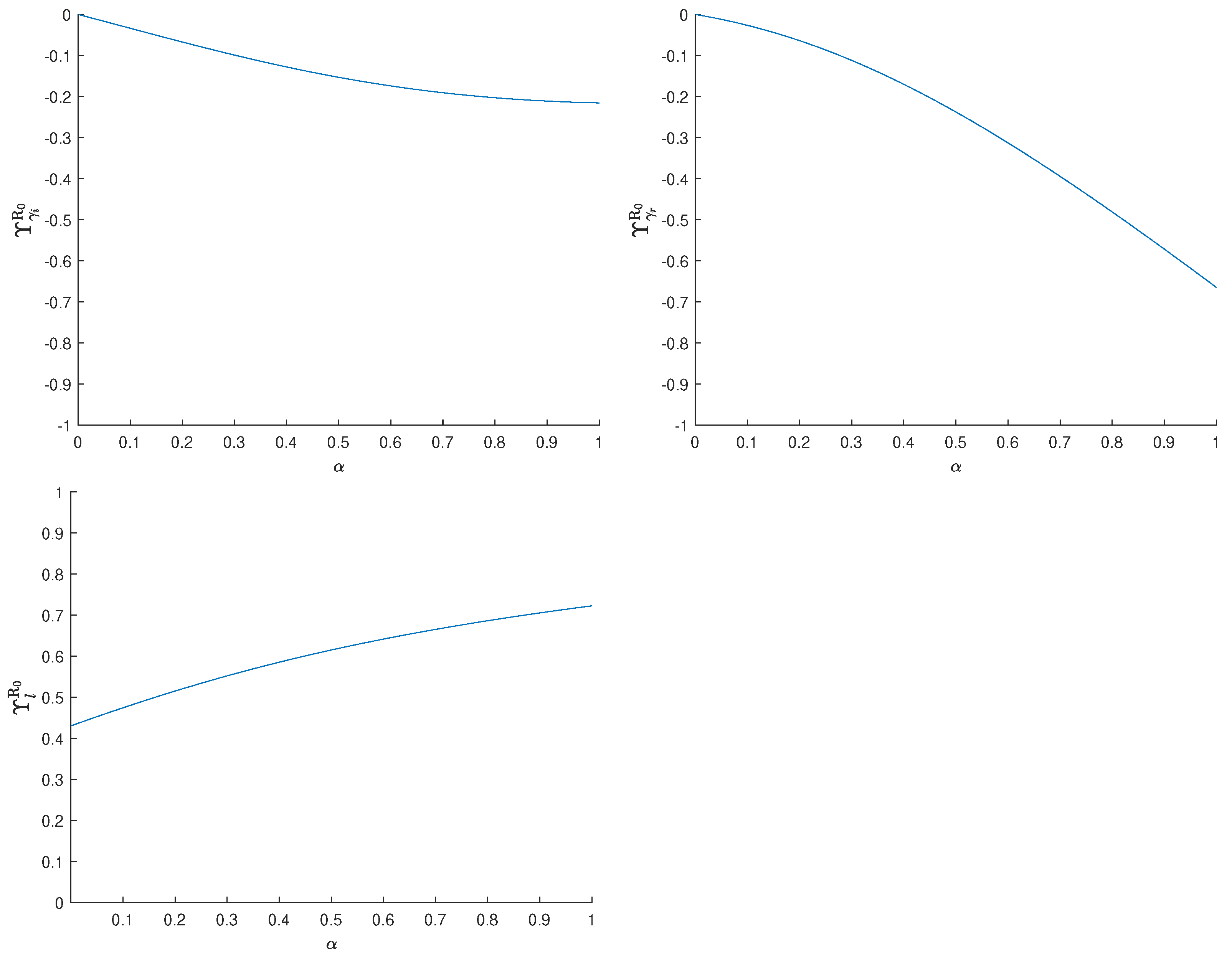
In the general situation of our fractional-order model (2), it should be emphasized that the sensitivity depends on the derivative order α of the fractional operator. We can observe this in Figure 5, where one clearly sees that the variation of α influences the sensitivity index of parameters β , ρ 1 , γ i , γ r , and l.
We see in Figure 5 that the sensitivity indexes of β and ρ 1 exhibit a quite similar evolution with respect to α , being very sensitive to the variation of α . On the opposite side, the sensitivity indexes of γ i and l are much less sensitive to the variation of the fractional-order α . The graphics with respect to the remaining parameters of the model are omitted here because, using the same scale, their curves do not go far from the x-axis.
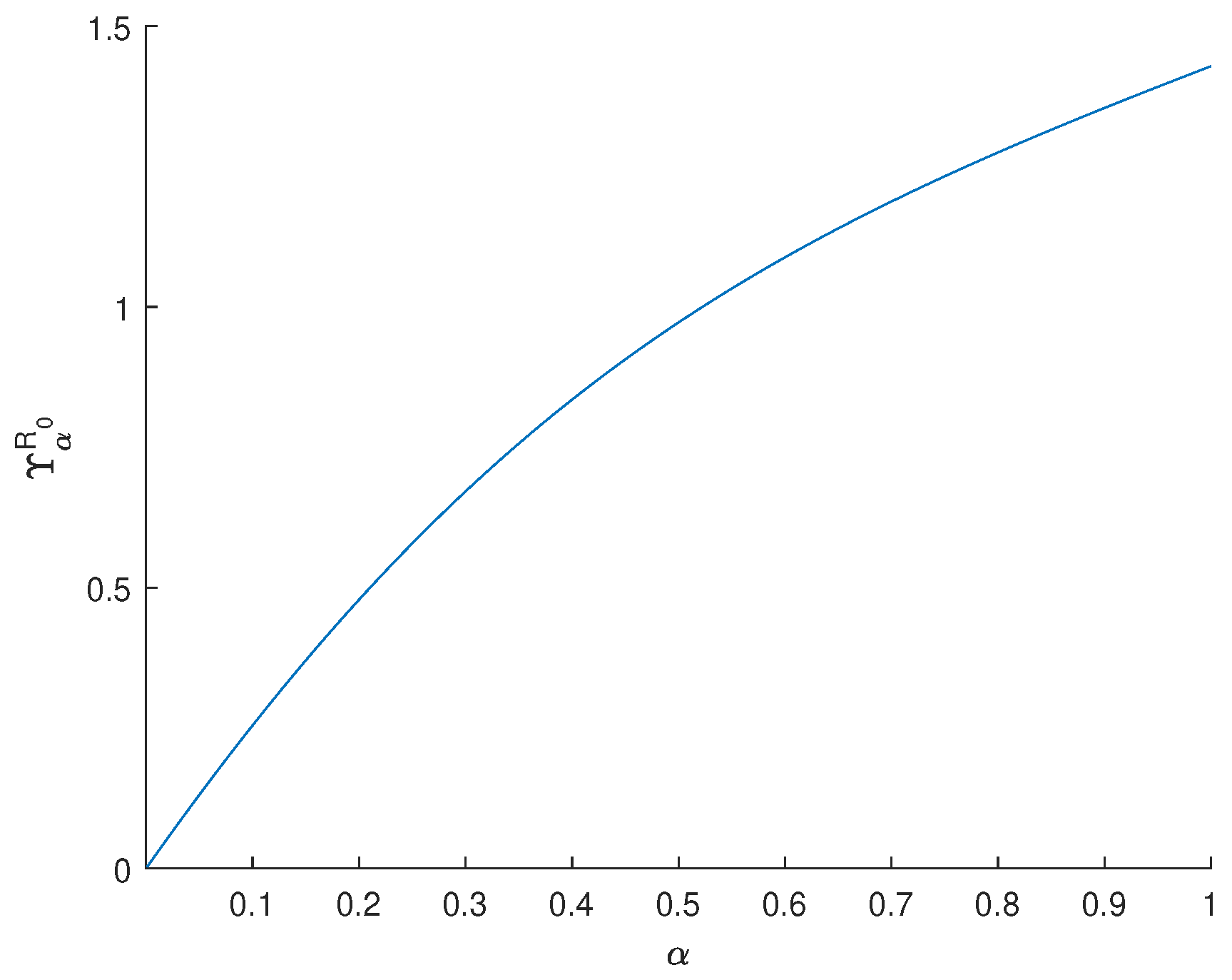
The evolution of the sensitivity index for the basic reproduction number R 0 with the variation of the derivative order α is presented in Figure 6. We observe that the sensitivity index decreases with the decrease of α .
Figure 5 and Figure 6 also show that the sensitivity of the model decreases in absolute value with the decrease in the derivative order. This means that the fractional-order model is less sensitive than the classical one, which is an advantage of our model.

3.3. Fractional Optimal Control of the Model

In this section, we aim to minimize the number of COVID-19-infected individuals and reduce the cost of control measures. This is carried out through (i) the use of vaccination as an effective measure time-dependent control v ( t ) and (ii) the use of the preventive measure control m ( t ) (representing the use of masks, limitations of the number of individuals in closed confined spaces, etc.), in order to control person-to-person contact. Therefore, the following fractional-order optimal control problem is considered:
min J ( I , P , v , m ) = 0 t f k 1 I + k 2 P + k 3 v 2 + k 4 m 2 d t
subject to
0 C D t α S = β α ( 1 m ) I S N l β α ( 1 m ) H S N β α ( 1 m ) P S N v S , 0 C D t α E = β α ( 1 m ) I S N + l β α ( 1 m ) H S N + β α ( 1 m ) P S N κ α E , 0 C D t α I = κ α ρ 1 E ( γ a α + γ i α ) I δ i α I , 0 C D t α P = κ α ρ 2 E ( γ a α + γ i α ) P δ p α P , 0 C D t α A = κ α ( 1 ρ 1 ρ 2 ) E , 0 C D t α H = γ a α ( I + P ) γ r α H δ h α H , 0 C D t α R = γ i α ( I + P ) + γ r α H + v S , 0 C D t α F = δ i α I + δ p α P + δ h α H ,
with given initial conditions
S ( 0 ) , E ( 0 ) , I ( 0 ) , P ( 0 ) , A ( 0 ) , H ( 0 ) , R ( 0 ) , F ( 0 ) = S 0 , E 0 , I 0 , P 0 , A 0 , H 0 , R 0 , F 0 0 .
Parameters 0 < k 1 , , k 4 < + are positive numbers that balance the size of the linear and quadratic terms in the cost, and t f is the duration of the control program. Moreover, k 3 and k 4 represent the costs of applying the control measures v and m, respectively. The set of admissible control functions is
U = ( v ( · ) , m ( · ) ) L ( 0 , t f ) : 0 v ( t ) v max , 0 m ( t ) m max t ( 0 , t f ) .
Pontryagin’s minimum principle (PMP) for fractional optimal control [18] is used to determine the solution of the problem. The Hamiltonian associated with our optimal control problem is given by
H = k 1 I + k 2 P + k 3 v 2 + k 4 m 2 + ξ 1 ( β α ( 1 m ) I S N l β α ( 1 m ) H S N β α ( 1 m ) P S N v S ) + ξ 2 ( β α ( 1 m ) I S N + l β α ( 1 m ) H S N + β α ( 1 m ) P S N κ α E ) + ξ 3 ( κ α ρ 1 E ( γ a α + γ i α ) I δ i α I ) + ξ 4 ( κ α ρ 2 E ( γ a α + γ i α ) P δ p α P ) + ξ 5 ( κ α ( 1 ρ 1 ρ 2 ) E ) + ξ 6 ( γ a α ( I + P ) γ r α H δ h α H ) + ξ 7 ( γ i α ( I + P ) + γ r α H + v S ) + ξ 8 ( δ i α I + δ p α P + δ h α H )
and the adjoint system of PMP asserts that the co-state variables ξ i ( t ) , i = 1 , , 8 , satisfy
0 C D t α ξ 1 ( t ) = ( m 1 ) ( β α ( I + l H ) + β α P ) ( ξ 1 ξ 2 ) N + ( ξ 7 ξ 1 ) v , 0 C D t α ξ 2 ( t ) = κ α ( ξ 2 + ξ 3 ρ 1 + ξ 4 ρ 2 ξ 5 ( ρ 1 + ρ 2 1 ) ) , 0 C D t α ξ 3 ( t ) = k 1 ( γ a α + γ i α ) ξ 3 + γ a α ξ 6 + γ i α ξ 7 + δ i α ( ξ 8 ξ 3 ) + β α ( m 1 ) ( ξ 1 ξ 2 ) S N , 0 C D t α ξ 4 ( t ) = k 2 ( γ a α + γ i α ) ξ 4 + γ a α ξ 6 + γ i α ξ 7 + δ p α ( ξ 8 ξ 4 ) + β α ( m 1 ) ( ξ 1 ξ 2 ) S N , 0 C D t α ξ 5 ( t ) = 0 C D t α ξ 7 ( t ) = 0 C D t α ξ 8 ( t ) = 0 , 0 C D t α ξ 6 ( t ) = γ r α ( ξ 7 ξ 6 ) + δ h α ( ξ 8 ξ 6 ) l β α ( m 1 ) ( ξ 1 ξ 2 ) S N ,
with t = t f t . In turn, the minimality conditions of PMP establish that the optimal controls v * and m * are given by
v * ( t ) = min max 0 , ( ξ 1 ( t ) ξ 7 ( t ) ) S ( t ) 2 k 3 , v max , m * ( t ) = min max 0 , ( β α ( I ( t ) + l H ( t ) ) + β α P ( t ) ) ( ξ 2 ( t ) ξ 1 ( t ) ) S ( t ) 2 k 4 N , m max .
Finally, according to PMP, the following transversality conditions also hold true:
ξ i ( t f ) = 0 , i = 1 , , 8 .
In Section 3.4, we use the necessary optimality conditions (9)–(11) to numerically solve the optimal control problem (4)–(7), both in classical and fractional cases.

3.4. Numerical Results and Cost-Effectiveness of the Fractional Optimal Control Problem

Pontryagin Minimum Principle (PMP) is utilized to numerically solve the optimal control problem as discussed in Section 3.3. For that we use the predict-evaluate-correct-evaluate (PECE) method of Adams–Basforth–Moulton [19], implemented by us in MATLAB. Firstly, we solve System (5) by the PECE procedure, with the initial values for the state variables (6) given, and a guess for the controls over the time interval [ 0 , t f ] , thus obtaining the values of the state variables. Analogously to [20], a change in variables is employed in the adjoint system and in the transversality conditions, obtaining a fractional initial value problem (IVP) from (9)–(11). The resulting IVP is also solved with the PECE algorithm, and the values of the co-state variables ξ i , i = 1 , , 8 , are obtained. The controls are then updated by a convex combination of the controls of the previous iteration and the current values, computed according to (10). This procedure is iteratively repeated until the values of all the variables and the values of the controls are almost coincident with the ones of the previous iteration, that is, until convergence is achieved. The solutions of the classical model (i.e., the case α = 1 ) were successfully confirmed by a classical forward-backward scheme, also implemented by us in MATLAB.
As estimated in [21], we consider that 10% of infected individuals are super-spreaders.
According with [22], the initial number of asymptomatic persons is estimated to be
I 0 + P 0 0.15 .
In what follows, we assume that the total population is equal to 10,280,000 (N). Based on real data obtained from [13] and on the above assumptions, the initial conditions are R 0 = 278776 , E 0 = 92069 , P 0 = 68208 × 0.1 , I 0 = 68208 × 0.9 , A 0 = 68208 / 0.15 , F 0 = 34 , H 0 = 2366 and S 0 = N R 0 E 0 P 0 I 0 A 0 H 0 .
The maximum number of effective daily vaccinated is estimated to be 30,000 (60,000 vaccine doses for two-dose vaccines), which corresponds to 0.003 in percentage, and this is the value of v max .
In addition, we consider that the maximum rate of reduction in contacts is the maximum value of function m ( t ) , m max , exhibited in Figure 2 and considered during the modelling phase.
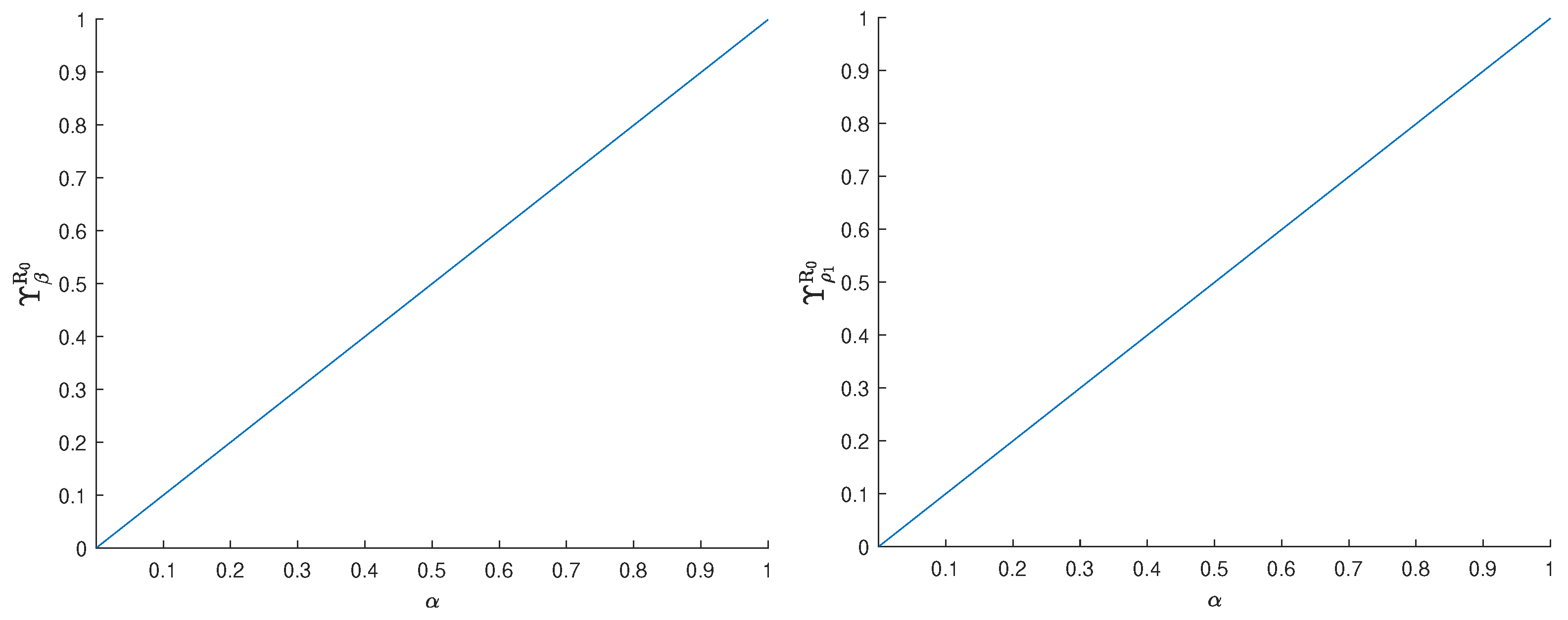
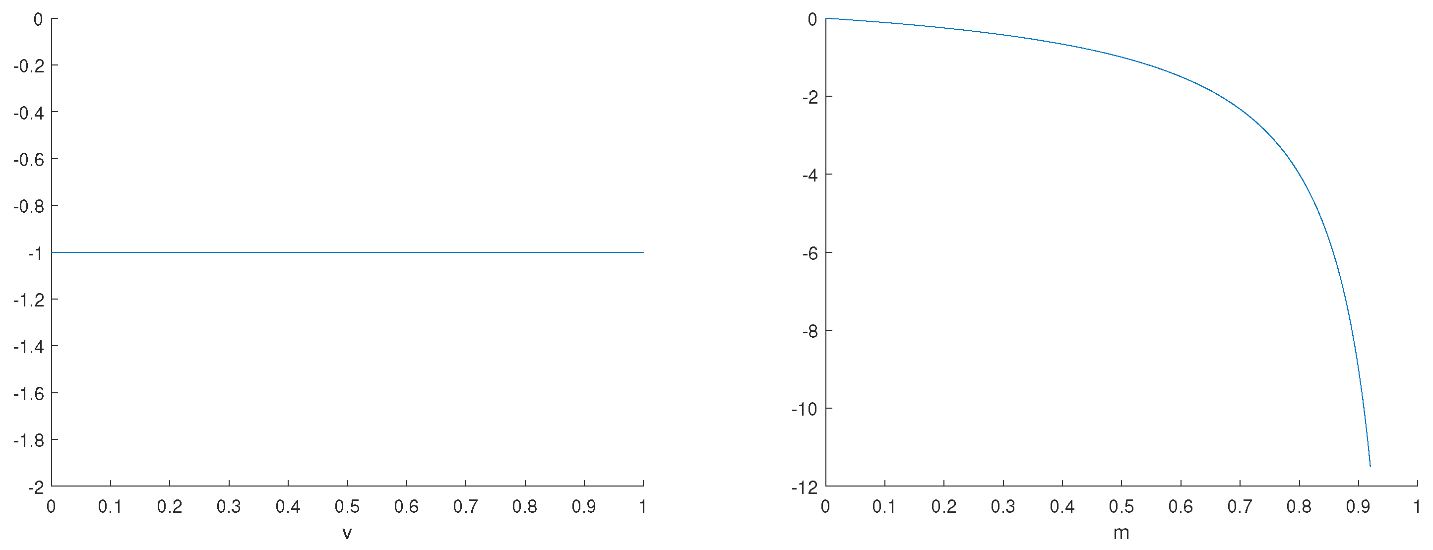
Following [23], the relevance of the two control measures considered in the control of the disease is calculated using the sensitivity index, as presented in Definition 1. With this purpose, the basic reproduction number of the model, now incorporating the two controls, needs to be determined. For that, we look to the controls as parameters. Using the next-generation matrix method of [24], we obtain that the basic reproduction number is now given by
R 0 = ( a h + γ a α l ) β α ( m 1 ) ρ 1 a h a i v + ( a h β α + β α γ a α l ) ( m 1 ) ρ 2 a h a p v ,
where a i = γ a α + γ i α + δ i α , a p = γ a α + γ i α + δ p α , and a h = γ r α + δ h α . The sensitivity indices are presented as functions of the control parameters in Figure 7, using the parametric values from Table 1 and the classical derivative.
The plots of Figure 7 show the following: (i) the curve of vaccination is constant and equal to 1 , meaning that the vaccination program has a substantial impact, even for small rates of application; (ii) the curve of preventive measures rapidly moves away from zero, meaning that a preventive programme has a substantial impact only if its rate of application is high. Thus, the use of masks and the limitation of individuals in confined spaces (shops, schools, and other public spaces) have to be mandatory and should be monitored by the authorities, when it is possible.
The weights of the cost functional (4) balance the relative importance of quadratic control terms. Since super-spreaders have a greater impact in the dynamics of the disease, we consider that super-spreaders are more expensive to control than regular infected individuals. Because the preventive measures need a high rate of application to be effective, we consider that preventive measures are more expensive than vaccination. In our numerical experiments, weights are k 1 = 1 , k 2 = 5 , k 3 = 1 , and k 4 = 10 .
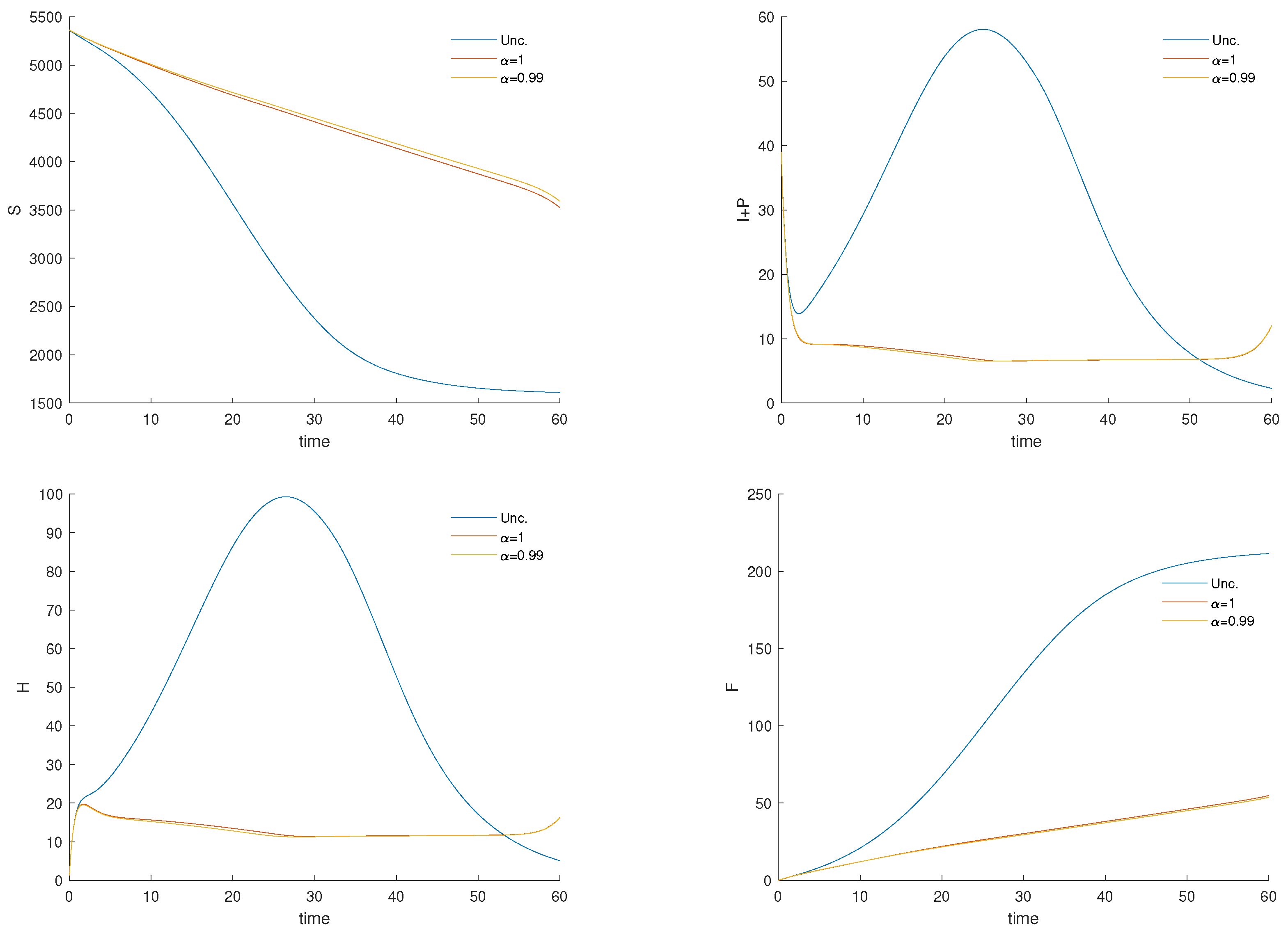
In Figure 8, the trajectories of the fractional optimal control problem (FOCP) for α = 0.99 are exhibited along with the solution of the classical optimal control problem (i.e., with α = 1 ) and the original (uncontrolled) model (2).
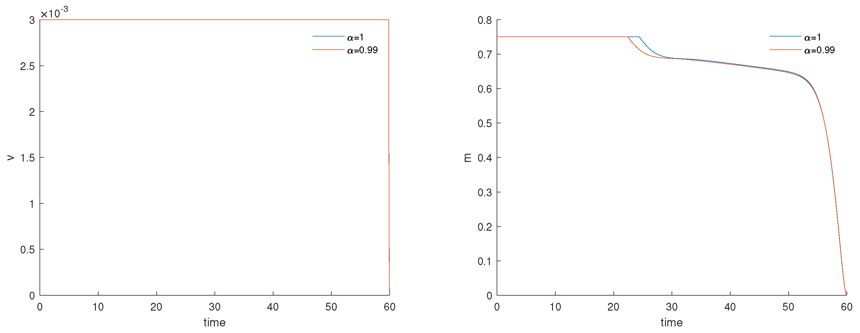
The corresponding Pontryagin controls are shown in Figure 9.
We can see in Figure 8 and Figure 9 that a change in the value of α corresponds to variations in the state and control variables. Moreover, comparing the solution of the original/uncontrolled model with the solution of the optimal control problem obtained from the application of the Pontryagin principle, we conclude that the considered control measures are effective in the management of COVID-19.
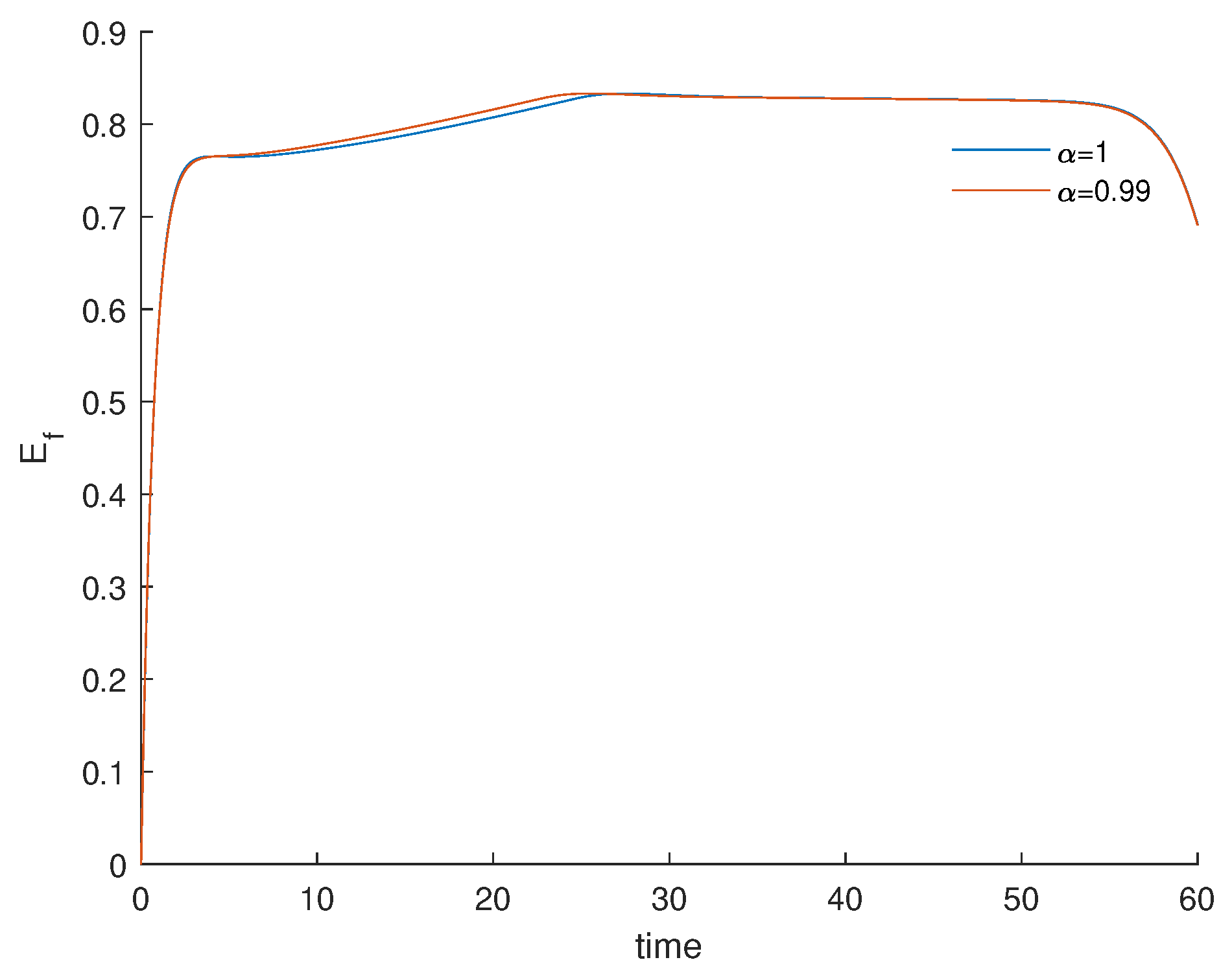
Figure 10 exhibits the efficacy function, defined in [25] by
E f ( t ) = i ( 0 ) i * ( t ) i ( 0 ) = 1 i * ( t ) i ( 0 ) ,
where i * ( t ) = I * ( t ) + P * ( t ) is the optimal solution associated with the fractional optimal control, and i ( 0 ) = I ( 0 ) + P ( 0 ) is the correspondent initial condition.
The efficacy function E f ( t ) measures the proportional variation in the number of infected individuals after the application of the control measures, { v * , m * } , by comparing the number of infectious individuals at time t with its initial value i ( 0 ) .
To assess the cost and the effectiveness of the proposed fractional control measures during the intervention period, some summary measures are now presented.
The total cases averted by the intervention during the time period t f is defined by
A V = t f i ( 0 ) 0 t f i * ( t ) d t ,
where i * ( t ) is the optimal solution associated with the fractional optimal controls, and i ( 0 ) is the correspondent initial condition [25]. Note that this initial condition is obtained as the equilibrium proportion i ¯ of System (2), which is independent of time, so that t f i ( 0 ) = 0 t f i ¯ d t represents the total infectious cases over a given period of t f days.
Effectiveness is defined as the proportion of cases averted to the total cases possible under no intervention [25]:
F ¯ = A V i ( 0 ) t f = 1 0 t f i * ( t ) d t i ( 0 ) t f .
The total cost associated with the intervention is defined in [25] by
T C = 0 t f C 1 v * ( t ) s * ( t ) + C 2 m * ( t ) i * ( t ) d t ,
where s * ( t ) = S * ( t ) , and C i corresponds to the per person unit cost of the two possible interventions: (i) vaccination at time t of susceptible individuals ( C 1 ) and (ii) the implementation of preventive measures, such as the use of masks and the physical distancing of susceptible individuals ( C 2 ).
Finally, the average cost-effectiveness ratio is given by
A C E R = T C A V
(see [25,26]).
Table 3 summarizes the presented cost-effectiveness measures (13)–(17). The results clearly show the effectiveness of the controls in the reduction of COVID-19 infections and the advantage of using the fractional model.
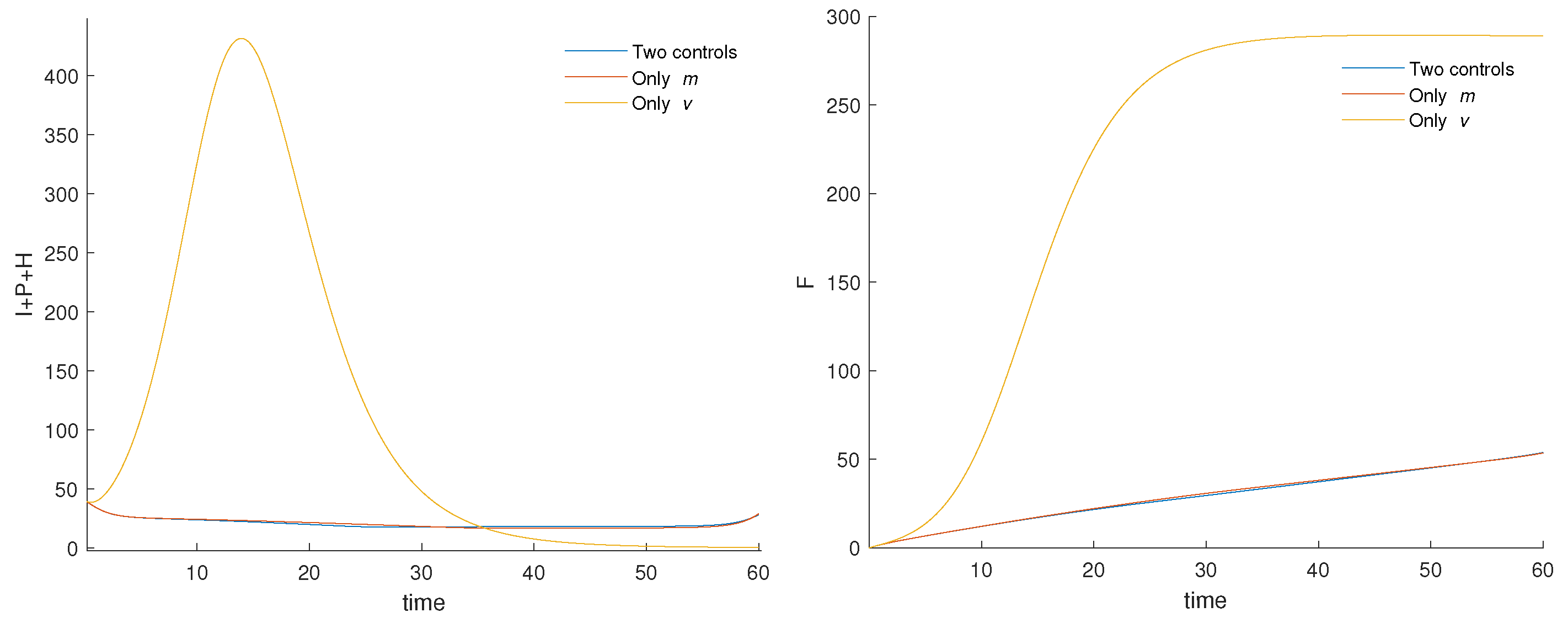
To conclude, Figure 11 exhibits the dynamics of the infected population, I + P + H , and of fatalities, F, in three scenarios: (i) when the two controls are used; (ii) when only control m is used ( v = 0 ); and (iii) when only control v is used ( m = 0 ). Due to low vaccination rates, considering v = 0 , one obtains almost the same solution as the one obtained using both controls. On the other hand, erasing preventive measures leads to a serious healthcare problem. Preventive measures are in this case more effective than vaccination.

4. Conclusions

A classical compartmental model with super-spreaders was firstly proposed and applied to provide an estimation of infected individuals and deaths in Wuhan, China, in [9], and this model was later extended to the fractional-order case in order to include memory effects and better describe the realities of Spain and Portugal [6]. Unfortunately, the fractional-order model of [6] is inconsistent, in the sense that it does not satisfy appropriate time dimensions. Here, the fractional model of [6] was corrected and then used, for the first time in the literature, to model the third wave of the COVID-19 pandemic in Portugal, which occurred between 27 December 2020 and 16 February 2021. Our data fitting consisted in the minimization of the l 2 norm of the difference between the real values reported from the Health Authorities and the predictive cases of COVID-19 infection given by our model (2), showing that, in terms of absolute errors, the fractional-order model is better than the classical integer-order one. Another advantage of the fractional-order model was found from a sensitivity analysis, measuring the importance of each parameter in COVID-19 transmission, which allowed us to show that the sensitivity of the model decreases in absolute value with the decrease in the fractional-order α of differentiation, i.e., the fractional-order model is less sensitive to disturbances in the parameters than the classical one. Moreover, we introduced into the corrected model the use of vaccination and preventive control measures, investigating the use of fractional-order optimal control theory to minimize the number of COVID-19-infected individuals and reduce the associated costs. A post-optimal cost-effectiveness analysis has shown the effectiveness of controls to combat COVID-19 and the advantage of using the fractional-order model. Finally, it is shown that preventive measures are essential in the control of the pandemic.
The model investigated here is deterministic. For future work, it would be interesting to take into account the effect of noise. For integer-order models, one can refer to the works [27,28], where some COVID-19 stochastic differential equations are proposed that take into account noises derived from environmental fluctuations. Fractional stochastic models for COVID-19 are scarce and still need further investigations.

Author Contributions

Conceptualization, S.R. and D.F.M.T.; software, S.R.; validation, D.F.M.T.; formal analysis, S.R. and D.F.M.T.; investigation, S.R. and D.F.M.T.; writing—original draft preparation, S.R. and D.F.M.T.; writing—review and editing, S.R. and D.F.M.T. All authors have read and agreed to the published version of the manuscript.

Funding

This research was funded by The Portuguese Foundation for Science and Technology (FCT—Fundação para a Ciência e a Tecnologia) through projects UIDB/50008/2020 (Rosa) and UIDB/04106/2020 (Torres).

Institutional Review Board Statement

Not applicable.

Informed Consent Statement

Not applicable.

Data Availability Statement

The data supporting the reported results are public and can be found in [13,14].

Acknowledgments

The authors are very grateful to two referees for several constructive remarks and questions that helped them to improve the manuscript.

Conflicts of Interest

The authors declare that there is no conflict of interest. The funders had no role in the design of the study, in the collection, analyses, or interpretation of data, in the writing of the manuscript, or in the decision to publish the results.

References

  1. World Health Organization. Available online: https://www.who.int/emergencies/diseases/novel-coronavirus-2019/interactive-timeline# (accessed on 7 July 2021).
  2. Agarwal, P.; Nieto, J.J.; Ruzhansky, M.; Torres, D.F.M. Analysis of Infectious Disease Problems (COVID-19) and Their Global Impact; Infosys Science Foundation Series in Mathematical Sciences; Springer: Singapore, 2021. [Google Scholar]
  3. Bracher, J.; Wolffram, D.; Deuschel, J.; Görgen, K.; Ketterer, J.L.; Ullrich, A.; Schienle, M. A pre-registered short-term forecasting study of COVID-19 in Germany and Poland during the second wave. Nat. Commun. 2021, 12, 5173. [Google Scholar] [CrossRef] [PubMed]
  4. Ghaffari, V.; Mobayen, S.; Din, S.U.; Bartoszewicz, A.; Jahromi, A.T. A Robust H fault tolerant controller for uncertain systems described by linear fractional transformation model. IEEE Access 2021, 9, 104749–104760. [Google Scholar] [CrossRef]
  5. Jajarmi, A.; Baleanu, D.; Zarghami Vahid, K.; Mobayen, S. A general fractional formulation and tracking control for immunogenic tumor dynamics. Math. Meth. Appl. Sci. 2022, 45, 667–680. [Google Scholar] [CrossRef]
  6. Ndaïrou, F.; Area, I.; Nieto, J.J.; Silva, C.J.; Torres, D.F.M. Fractional model of COVID-19 applied to Galicia, Spain and Portugal. Chaos Solitons Fractals 2021, 144, 110652. [Google Scholar] [CrossRef] [PubMed]
  7. Bushnaq, S.; Saeed, T.; Torres, D.F.M.; Zeb, A. Control of COVID-19 dynamics through a fractional-order model. Alex. Eng. J. 2021, 60, 3587–3592. [Google Scholar] [CrossRef]
  8. Podlubny, I. Fractional Differential Equations. In Mathematics in Science and Engineering; Academic Press, Inc.: San Diego, CA, USA, 1999; Volume 198. [Google Scholar]
  9. Ndaïrou, F.; Area, I.; Nieto, J.J.; Torres, D.F.M. Mathematical modeling of COVID-19 transmission dynamics with a case study of Wuhan. Chaos Solitons Fractals 2020, 135, 109846. [Google Scholar] [CrossRef] [PubMed]
  10. Ndaïrou, F.; Area, I.; Bader, G.; Nieto, J.J.; Torres, D.F.M. Corrigendum to ‘Mathematical Modeling of COVID-19 Transmission Dynamics with a Case Study of Wuhan’ [Chaos Solitons Fractals 135 (2020), 109846]. Chaos Solitons Fractals 2020, 141, 110311. [Google Scholar] [CrossRef] [PubMed]
  11. Almeida, R. Analysis of a fractional SEIR model with treatment. Appl. Math. Lett. 2018, 84, 56–62. [Google Scholar] [CrossRef]
  12. Carvalho, A.R.M.; Pinto, C.M.A. Immune response in HIV epidemics for distinct transmission rates and for saturated CTL response. Math. Model. Nat. Phenom. 2019, 14, 307. [Google Scholar] [CrossRef]
  13. DGS—COVID-19. Ponto de situação atual em Portugal. Available online: https://covid19.min-saude.pt/ponto-de-situacao-atual-em-portugal/ (accessed on 30 October 2021).
  14. Dados Relativos à Pandemia COVID-19 em Portugal. Available online: https://github.com/dssg-pt/covid19pt-data (accessed on 30 October 2021).
  15. Rosa, S.; Torres, D.F.M. Parameter estimation, sensitivity analysis and optimal control of a periodic epidemic model with application to HRSV in Florida. Stat. Optim. Inf. Comput. 2018, 6, 139–149. [Google Scholar] [CrossRef] [Green Version]
  16. Chitnis, N.; Hyman, J.M.; Cushing, J.M. Determining important parameters in the spread of malaria through the sensitivity analysis of a mathematical model. Bull. Math. Biol. 2008, 70, 1272–1296. [Google Scholar] [CrossRef]
  17. Rodrigues, H.S.; Monteiro, M.T.T.; Torres, D.F.M. Sensitivity analysis in a dengue epidemiological model. In Conference Papers in Science; Hindawi: London, UK, 2013; Volume 2013. [Google Scholar]
  18. Almeida, R.; Pooseh, S.; Torres, D.F.M. Computational Methods in the Fractional Calculus of Variations; Imperial College Press: London, UK, 2015. [Google Scholar]
  19. Diethelm, K.; Ford, N.J.; Freed, A.D.; Luchko, Y. Algorithms for the fractional calculus: A selection of numerical methods. Comput. Methods Appl. Mech. Eng. 2005, 194, 743–773. [Google Scholar] [CrossRef] [Green Version]
  20. Rosa, S.; Torres, D.F.M. Optimal control of a fractional order epidemic model with application to human respiratory syncytial virus infection. Chaos Solitons Fractals 2018, 117, 142–149. [Google Scholar] [CrossRef] [Green Version]
  21. Cave, E. COVID-19 super-spreaders: Definitional quandaries and implications. Asian Bioeth. Rev. 2020, 12, 235–242. [Google Scholar] [CrossRef] [PubMed]
  22. Lemos-Paião, A.P.; Silva, C.J.; Torres, D.F.M. A new compartmental epidemiological model for COVID-19 with a case study of Portugal. Ecol. Complex. 2020, 44, 100885. [Google Scholar] [CrossRef]
  23. Panja, P. Optimal Control Analysis of a Cholera Epidemic Model. Biophys. Rev. Lett. 2019, 14, 27–48. [Google Scholar] [CrossRef] [Green Version]
  24. van den Driessche, P.; Watmough, J. Reproduction numbers and sub-threshold endemic equilibria for compartmental models of disease transmission. Math. Biosci. 2002, 180, 29–48. [Google Scholar] [CrossRef]
  25. Rodrigues, P.; Silva, C.J.; Torres, D.F.M. Cost-effectiveness analysis of optimal control measures for tuberculosis. Bull. Math. Biol. 2014, 76, 2627–2645. [Google Scholar] [CrossRef]
  26. Okosun, K.O.; Rachid, O.; Marcus, N. Optimal control strategies and cost-effectiveness analysis of a malaria model. BioSystems 2013, 111, 83–101. [Google Scholar] [CrossRef] [PubMed]
  27. Zine, H.; Boukhouima, A.; Lotfi, E.M.; Mahrouf, M.; Torres, D.F.M.; Yousfi, N. A stochastic time-delayed model for the effectiveness of Moroccan COVID-19 deconfinement strategy. Math. Model. Nat. Phenom. 2020, 15, 50. [Google Scholar] [CrossRef]
  28. Mahrouf, M.; Boukhouima, A.; Zine, H.; Lotfi, E.M.; Torres, D.F.M.; Yousfi, N. Modeling and forecasting of COVID-19 spreading by delayed stochastic differential equations. Axioms 2021, 10, 18. [Google Scholar] [CrossRef]
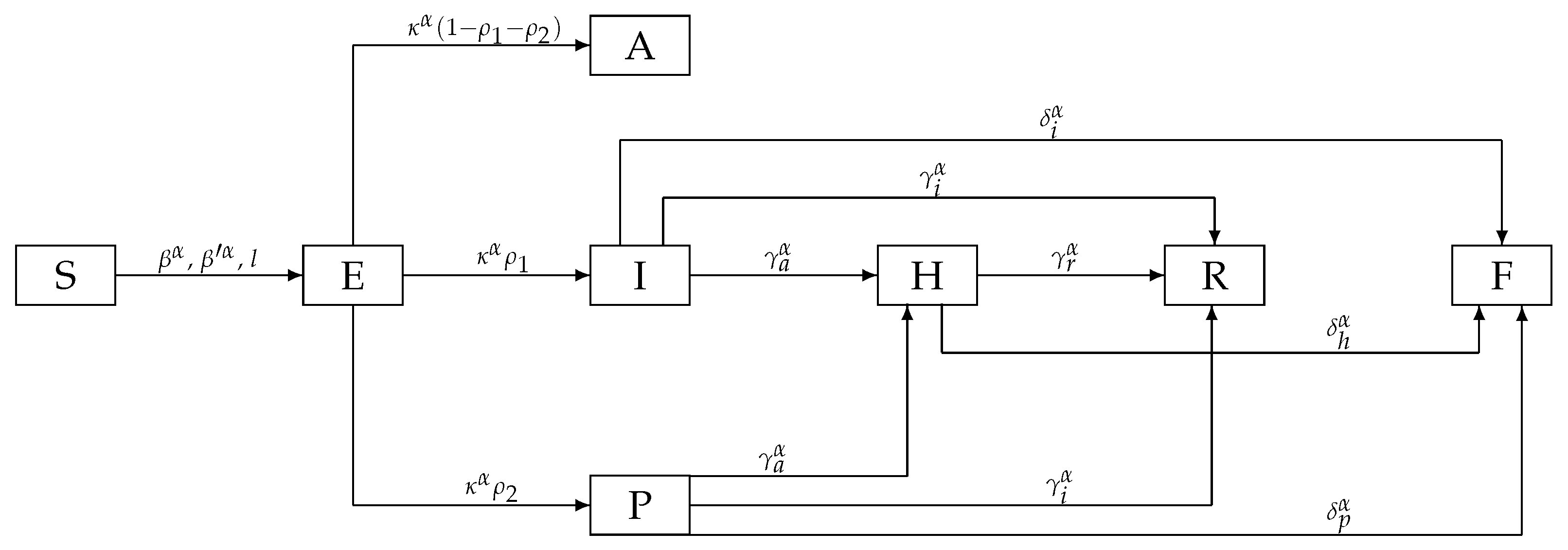
Figure 1. Flow diagram of the disease dynamics according to Model (2).
Axioms 11 00170 g001
Figure 2. Evolution function m ( t ) .
Axioms 11 00170 g002
Figure 3. (left) The number of confirmed cases per day in Portugal versus the ones predicted by Model (2) with parameters given by Table 1. The blue line corresponds to the real data ( I + P + H ) and the remaining lines have been obtained solving numerically the system of fractional differential equations (2). (right) The difference between the number of confirmed cases per day and the number of estimated cases, the solution of (2).
Axioms 11 00170 g003
Figure 4. Impact of the variation of the derivative order, α , in the evolution of the basic reproduction number R 0 of the COVID-19 model (2).
Axioms 11 00170 g004
Figure 5. Impact of the variation of α in the sensitivity indexes of β , ρ 1 , γ i , γ r , and l, in agreement with Definition 1.
Axioms 11 00170 g005aAxioms 11 00170 g005b
Figure 6. The sensitivity of Model (2) with respect to the fractional order of differentiation α , in agreement with Definition 1.
Axioms 11 00170 g006
Figure 7. Sensitivity index of the basic reproduction number (12) with respect to the control variables v (left) and m (right).
Axioms 11 00170 g007
Figure 8. Evolution of susceptible individuals S (top left), symptomatic infected individuals I + P (top right), hospitalized individuals H (bottom left), and fatalities F (bottom right) for the solutions of the uncontrolled model (2) and the optimal solutions of the FOCP (4)–(7) with fractional-order derivatives α = 1.0 and α = 0.99 and the parameter values of Table 1.
Axioms 11 00170 g008
Figure 9. Pontryagin controls v (left) and m (right) for the FOCP (4)–(7) using the values in Table 1 and fractional order derivatives α = 1.0 and α = 0.99 . The extremal controls v take their maximum value v max almost everywhere.
Axioms 11 00170 g009
Figure 10. Evolution of the efficacy function (13) for the FOCP (4)–(7) with values in Table 1 and fractional-order derivatives α = 1.0 and α = 0.99 .
Axioms 11 00170 g010
Figure 11. Comparison of the solution of the FOCP (4)–(7) with the fractional-order derivative α = 0.99 , considering the two controls with the two other cases where there is only one control used. (left) Variation of infected individuals I + P + H . (right) Evolution of fatalities F.
Axioms 11 00170 g011
Table 1. Description and values of the parameters of Model (1) taken from [9,10].
NameDescriptionValue
β human-to-human transmission coefficient2.55
ltransmissibility of hospitalized patients1.56
β transmission coefficient of super-spreaders7.65
κ rate at which an individual leaves the exposed0.25
class to become infectious
ρ 1 proportion of progression from class E0.58
to symptomatic infectious class I
ρ 2 rate at which exposed ind. become super-spreaders0.001
γ a rate at which symptomatic and super-spreaders0.94
become hospitalized
γ i recovery rate without being hospitalized0.27
γ r recovery rate of hospitalized patients0.5
δ i disease induced death rate due to infected ind.1/23
δ p disease induced death rate due to super-spreader ind.1/23
δ h disease induced death rate due to hospitalized ind.1/23
Table 2. Results of model fitting.
Derivative OrdersAbsolute ErrorRelative Error (%)
1.021.08859514.13
0.9919.87813513.37
Table 3. Summary of cost-effectiveness measures (13)–(17) for classical ( α = 1 ) and fractional ( 0 < α < 1 ) COVID-19 disease optimal control problems. Parameters according to Table 1 and C 1 = C 2 = 1 in (16).
α A TC ACER F ¯
0.991870.081116.430.5969980.79967
1.01865.951114.530.5972960.79791
Publisher’s Note: MDPI stays neutral with regard to jurisdictional claims in published maps and institutional affiliations.