Abstract
Recently, a continuous-time compartmental mathematical model for the spread of the Coronavirus disease 2019 (COVID-19) was presented with Portugal as case study, from 2 March to 4 May 2020, and the local stability of the Disease Free Equilibrium (DFE) was analysed. Here, we propose an analogous discrete-time model and, using a suitable Lyapunov function, we prove the global stability of the DFE point. Using COVID-19 real data, we show, through numerical simulations, the consistence of the obtained theoretical results.
Keywords:
mathematical modelling; epidemiology; COVID-19 pandemic; qualitative theory; Lyapunov functions; numerical simulations with real data MSC:
65L12; 92D30
1. Introduction
The coronavirus belong to the family of Coronaviridae. It is a virus that causes infection to humans, other mammals and birds. The infection usually affects the respiratory system, and the symptoms may vary from simple colds to pneumonia. To date, eight coronaviruses are known. The new coronavirus SARS-CoV-2 originates COVID-19, and was identified for the first time in December 2019 in Wuhan, China. Two other coronaviruses have caused outbreaks: SARS-CoV, in 2002–2003, and MERS-CoV in 2012 [1]. The COVID-19 pandemic in an ongoing pandemic, probably the most significant one in human history. The effects are so severe that it has been necessary to use quarantining to control the spread. It has forced humans to adapt to this new situation [2].
The use of mathematical compartmental models to study the spread and consequences of infectious diseases have been used successfully for a long time. The techniques to study compartmental models are vast: continuous models, fractional models, and discrete models, among others [2]. The complexity of the models is determined by the effects and consequences of the disease. Several models have been proposed for COVID-19 spread; see [2,3,4,5], among others. In this work, we are interested in discretizing the model presented in [3], using the Mickens method [6,7], which was applied successfully in several different contexts [8].
In Section 2, we recall the SAIQH (susceptible–asymptomatic–infectious–quarantined–hospitalized) continuous-time mathematical model, the equilibrium points and the stability results of [3]. Section 3 is dedicated to the original results of our work: the new discrete-time model, the proof of its well-posedness, the computation of the equilibrium points, and the proof of the stability of the disease-free equilibrium point. We end Section 3 with numerical simulations showing the consistency of our results. Finally, Section 4 is dedicated to discussion of the obtained results and some possible future work directions.
2. Preliminaries
This section is dedicated to the presentation of the continuous-time model [3] and its results, which establish the stability of the equilibrium points. For more information, see [3].
The total living population under study at time is denoted by as follows:
where represents the susceptible individuals; the infected individuals without symptoms or with mild ones; the infected individuals; the individuals in quarantine, that is, in isolation at home; the hospitalized individuals; and, finally, the hospitalized individuals in intensive care units. There is another class that is also considered, , that gives the cumulative number of deaths due to COVID-19 for all . Regarding the parameters, all of them are positive. The recruitment rate into the susceptible class is ; all individuals of all classes are subject to the natural death rate along all time under study. Susceptible individuals may become infected with COVID-19 at the following rate:
where is the human-to-human transmission rate per unit of time (day) and and quantify the relative transmissibility of asymptomatic individuals and hospitalized individuals, respectively. The class does not enter in because the number of health care workers that become infected by SARS-CoV-2 in intensive care units is very low and can be neglected. A fraction of the susceptible population is in quarantine at home, at rate . Consequently, only a fraction of susceptible individuals are assumed to be able to become infected. Since there is uncertainty about long-immunity after recovery, it is assumed that individuals of class Q will become susceptible again at a rate . It is also considered that only a fraction of the quarantined individuals move from class Q to S. It means that of the quarantined individuals return to class S at the end of days. These assumptions are justified by the state of calamity that was immediately decreed by the government of Portugal to address the state of emergency, which was fully respected by the Portuguese population. After days of infection, only a fraction of infected individuals without (or with mild) symptoms have severe symptoms. Thus, of individuals of compartment A move to I at rate . A fraction of infected individuals with severe symptoms are treated at home and the other fraction are hospitalized, both at rate . The model considers the three following scenarios for hospitalized individuals:
- A fraction of individuals in class H can evolve to a state of severe health status, needing an invasive intervention, such as artificial respiration, so they need to move to intensive care, at rate ;
- A fraction of individuals in class H die due to COVID-19, the disease related death rate associated with hospitalized individuals being ;
- A fraction of individuals in class H recover and, consequently, return home in quarantine/isolation at rate .
Regarding the hospitalized individuals in intensive care units, the model considers two possibilities as follows:
- A fraction of individuals in class recover and move to the class H at rate ;
- A fraction of individuals in class die due to COVID-19, the disease-related death rate associated with hospitalized individuals in intensive care units being .
Compiling all the previous assumptions, one has the following mathematical model:

Table 1.
Description of the parameters and initial conditions of model (4).
In [3], it is shown that the biologically feasible region is given by the following:
which is positively invariant for (4) for all non-negative initial conditions. To simplify the expressions in the computations, the following notation is used:
- (i)
- ;
- (ii)
- ;
- (iii)
- ;
- (iv)
- ;
- (v)
- ;
- (vi)
- ;
- (vii)
- ;
- (viii)
- ;
- (ix)
- ;
- (x)
- .
Model (4) has the following reproduction number:
and two equilibrium points, the disease free equilibrium (DFE) point
and the endemic equilibrium (EE) point that is given by the following:
with
where . Assuming that the transmission rate is strictly positive, we have the following:
Regarding the stability of the equilibrium points, the following results hold.
Lemma 1
Lemma 2
3. Results
In this section, we begin by presenting our proposal for a COVID-19 discrete-time model. After that, we show the well-posedness of the model, that is, we prove that the solutions of the model are positive and bounded and that the equilibrium points coincide with those of the continuous-time model presented in Section 2. We finalize this section by proving the global stability of the disease-free equilibrium point, using a suitable Lyapunov function and with the presentation of some numerical simulations, using real data, showing the consistency of our theoretical results.
3.1. The Discrete-Time Model
One of the important features of the discrete-time epidemic models obtained by the Mickens method is that they present the same features of the corresponding original continuous-time models. Our nonstandard finite discrete difference (NSFD) scheme for solving (4) is a numerical dynamically consistent method based on [9]. Let us define the time instants with n integer, the step size as , and as the approximated values of the following:
Discretizing system (4) using the NSFD scheme, we obtain the following:
where the denominator function is [10]. Throughout this work, for brevity, we write .
Remark 1.
Let us consider the region . Our next lemma shows that the feasible region is equal to the continuous case.
Lemma 3.
Any solution ofof model (11) with positive initial conditions is positive and ultimately bounded in Ω.
Proof.
Since model (11) is linear in , we can rewrite it as the following:
Since all parameters of model (13) are positive and the initial conditions are also positive, then, by induction, , , , , and for all . Regarding the boundedness of the solutions, the total population . Adding all equations of (13), we obtain the following:
By Lemma 2.2 of Shi and Dong [11],
so, if , then for all . Thus, is the biologically feasible region. □
Solving in system (13) we can see that there exists two equilibrium points:
- The disease free equilibrium (DFE) point
- The endemic equilibrium (EE) pointwhere
and . In this point,
3.2. Global Stability
We now prove the global stability of (14).
Theorem 1.
For the discretized system, the DFE pointis globally stable if. If, then the DFE is unstable.
Proof.
Let us define the discrete Lyapunov function as the following:
Hence, for all , . Moreover, if and only if . Computing , we have the following:
where . Note that , for all , and if and only if . For each ,
Therefore,
From equations of system (11), we obtain the following:
and, at the disease-free equilibrium point , we have the following relations:
Substituting in , and simplifying, we obtain the following:
Let
Then,
Since
(22) is equal to the following:
Once more, from system (13) it can seen that , so
Therefore,
Hence, if , then for all , that is, is a monotone decreasing sequence. We have . Then there is a limit for . Therefore, implies that , , . So, if , then is globally asymptotically stable. □
3.3. Numerical Simulations
In this section, we show, numerically, that our discretized model describes well the transmission dynamics of COVID-19 in Portugal, from 2 March to 4 May 2020. Our data were obtained from the daily reports from DGS, available in [12], and since we consider the spread from 2 March, the initial time corresponds to 2 March 2020.
The initial values are the same as those used in [3]. Regarding the parameters, using [13], we can obtain the values from 2019, so the parameters were updated with respect to [3], but the difference is very small. All the values used in our simulations are presented in Table 2.
Table 2.
Parameter values and initial conditions of (4).
Using the values of Table 2, in Figure 1, we compare the number of infected individuals predicted by our discrete-time model, the ones predicted by the continuous model of [3], and the real data.
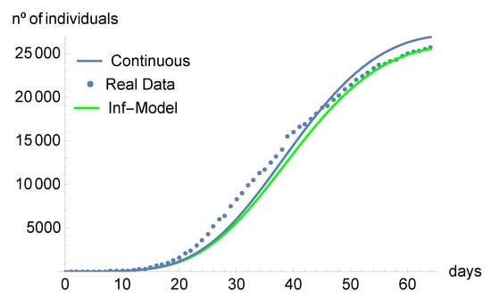
Figure 1.
Number of infected individuals predicted by the discrete-time model: solid green line. Real data: dotted line. Number of infected individuals predicted by the continuous model: solid blue line.
Figure 2 shows the consistency of our result. We compare the predictions from the continuous model with the predictions from the discrete-time model. Using the parameter values of Table 2, , the number of infected and asymptomatic individuals, as well as the ones in the hospital and intensive care units, tend to disappear. The susceptible individuals and those in quarantine tend to the equilibrium point as time increases.
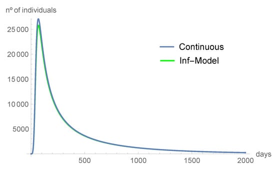
Figure 2.
The infected individuals tend to disappear with time.
Comparing the graphics from Figure 2, Figure 3, Figure 4, Figure 5, Figure 6 and Figure 7, we can see that the asymptotic behavior is similar. However, the discrete-time model predicts, in some instances, smaller values. All the computations were done using Mathematica, version 12.1.
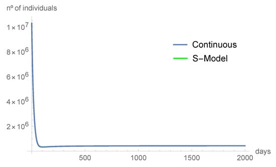
Figure 3.
The susceptible individuals tend quickly to .
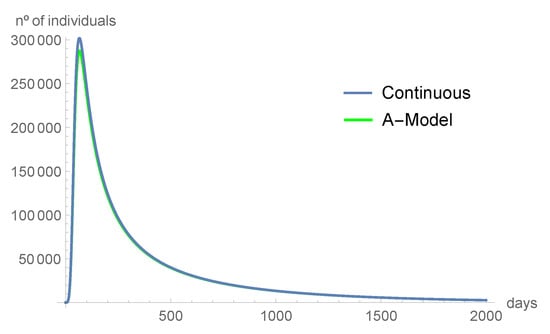
Figure 4.
The asymptomatic individuals tend to disappear with time.
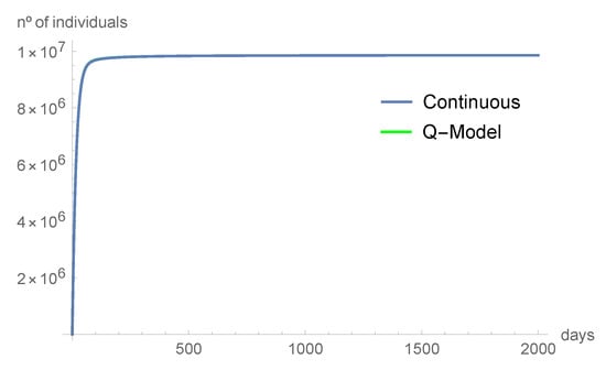
Figure 5.
The number of individuals in quarantine tend quickly to .
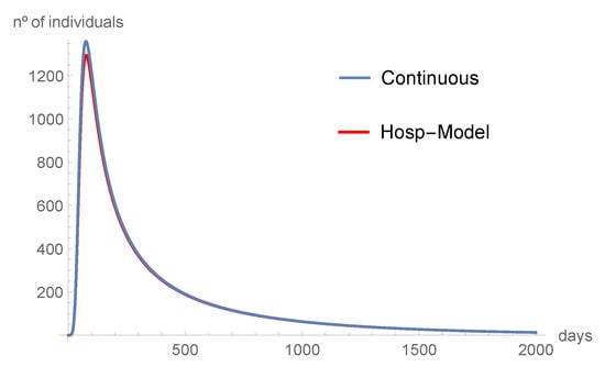
Figure 6.
The hospitalized individuals tend to disappear with time.
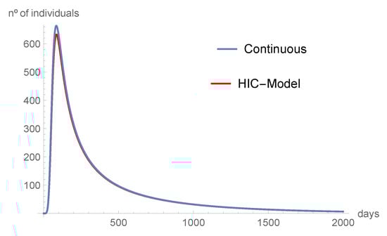
Figure 7.
The individuals in intensive care also tend to disappear with time.
4. Discussion
The COVID-19 pandemic has been a shocking experience to every human being, and no one expected the consequences felt worldwide. From this, we can also state that the number of variables and parameters to be taken into account in a COVID-19 model are not small. Indeed, if there is such thing as a good model that explains COVID-19, surely it is not a simple model. Moreover, most of the models that explain epidemiological, ecological, and economical phenomena are not linear. Therefore, given the tools available, it is impossible to present an exact solution to the problem. That is one of the reasons for the development of nonstandard finite difference methods. Indeed, such methods enable us to construct discrete models from continuous ones, allowing one to present numerical solutions.
Nowadays, there are several nonstandard finite schemes. We have used here the one developed by Mickens because it has shown to be dynamically consistent. Precisely, we discretized the continuous-time model presented and analyzed in [3]. With our discrete-time model, we analyzed the evolution of the COVID-19 pandemic in Portugal, from its beginning up to 4 May 2020. This choice allowed us to compare our results with those of [3]. We obtained the equilibrium points of the proposed discrete-time model, showing that they coincide with the ones from the continuous model. From the qualitative analysis point of view, we believe that it is important to prove the stability of the equilibrium points if the model describes real data, which is our case here. For this reason, Figure 2, Figure 3, Figure 4, Figure 5, Figure 6 and Figure 7 show the simulation results made over 2000 days: our intention is to show the stability of the model. Regarding the stability, it should be noted that, in contrast with [3], which only proves local stability, here, we have proved the global stability of the disease-free equilibrium (DFE) and attempted to do the same with the endemic equilibrium (EE) point. However, regarding the EE, we were not able to prove the global stability analytically, and the question remains open. Figure 1 compares the predictions of the continuous model with those of the discrete-time model. One concludes that the discrete-time model fits a little bit better to the real data. From Figure 2, Figure 3, Figure 4, Figure 5, Figure 6 and Figure 7, we present the convergence to the disease-free equilibrium point, using both continuous and discrete models. The asymptotic behavior is similar; the only difference worth mentioning is that the discrete-time model, in some small interval of time, predicts smaller values than the continuous one.
In this work, we restricted ourselves to the development of the pandemic in Portugal. We are aware that new models are emerging and, in a future work, we intend to analyze a model that fits the data of more than one country and region, possibly globally. This is under investigation and will be addressed elsewhere. Another line of research concerns models that take vaccination into account [18]. Here, vaccination is not considered because our model was created to explain the development of COVID-19 at the beginning of the pandemic. However, regarding vaccination, individuals do not become immune, so we think that we need to wait a little longer to see the development. It remains open the question of how to prove global stability for the endemic equilibrium.
Author Contributions
Conceptualization, S.V. and D.F.M.T.; methodology, S.V. and D.F.M.T.; software, S.V.; validation, S.V. and D.F.M.T.; formal analysis, S.V. and D.F.M.T.; investigation, S.V. and D.F.M.T.; writing—original draft preparation, S.V. and D.F.M.T.; writing—review and editing, S.V. and D.F.M.T.; visualization, S.V. All authors have read and agreed to the published version of the manuscript.
Funding
The authors were partially supported by the Portuguese Foundation for Science and Technology (FCT): Sandra Vaz through the Center of Mathematics and Applications of Universidade da Beira Interior (CMA-UBI), project UIDB/00212/2020; Delfim F. M. Torres through the Center for Research and Development in Mathematics and Applications (CIDMA) of University of Aveiro, project UIDB/04106/2020.
Institutional Review Board Statement
Not applicable.
Informed Consent Statement
Not applicable.
Data Availability Statement
The data and information used in this work are accessible to anyone and can be found in the following links: https://www.pordata.pt/Portugal (accessed on 16 September 2021); http://www.covid19.min-saude.pt (accessed on 16 September 2021); https://covid19.min-saude.pt/ponto-desituaçãoatual-em-portugal (accessed on 16 September 2021).
Acknowledgments
The authors are grateful to three reviewers for their several comments and suggestions.
Conflicts of Interest
The authors declare no conflict of interest.
References
- DGS, COVID-19. Available online: http://www.covid19.min-saude.pt (accessed on 16 September 2021).
- Agarwal, P.; Nieto, J.J.; Ruzhansky, M.; Torres, D.F.M. Analysis of Infectious Disease Problems (COVID-19) and Their Global Impact, Infosys Science Foundation Series in Mathematical Sciences; Springer: Singapore, 2021. [Google Scholar]
- Lemos-Paião, A.; Silva, C.; Torres, D.F.M. A new compartmental epidemiological model for COVID-19 with a case study of Portugal. Ecol. Complex. 2020, 44, 100885. [Google Scholar] [CrossRef]
- Ndaïrou, F.; Area, I.; Nieto, J.J.; Silva, C.J.; Torres, D.F.M. Fractional model of COVID-19 applied to Galicia, Spain and Portugal. Chaos Solitons Fractals 2021, 144, 110652. [Google Scholar] [CrossRef] [PubMed]
- Ndaïrou, F.; Torres, D.F.M. Mathematical Analysis of a Fractional COVID-19 Model Applied to Wuhan, Spain and Portugal. Axioms 2021, 10, 135. [Google Scholar] [CrossRef]
- Mickens, R.E. Nonstandard Finite Difference Models of Differential Equations; World Scientific Publishing Co., Inc.: River Edge, NJ, USA, 1994. [Google Scholar]
- Mickens, R.E. Nonstandard finite difference schemes for differential equations. J. Differ. Equ. Appl. 2002, 8, 823–847. [Google Scholar] [CrossRef]
- Vaz, S.; Torres, D.F.M. A dynamically-consistent nonstandard finite difference scheme for the SICA model. Math. Biosci. Eng. 2021, 18, 4552–4571. [Google Scholar] [CrossRef] [PubMed]
- Mickens, R.E. Dynamic consistency: A fundamental principle for constructing nonstandard finite difference schemes for differential equations. J. Differ. Equ. Appl. 2005, 117, 645–653. [Google Scholar] [CrossRef]
- Mickens, R.E. Calculation of denominator functions for nonstandard finite difference schemes for differential equations satisfying a positivity condition. Numer. Methods Partial. Differ. Equ. 2007, 23, 672–691. [Google Scholar] [CrossRef]
- Shi, P.; Dong, L. Dynamical behaviours of a discrete HIV-1 virus model with bilinear infective rate. Math. Meth. App. Sci. 2014, 37, 2271–2280. [Google Scholar] [CrossRef]
- DGS, Ponto de Situação Atual em Portugal. Available online: https://covid19.min-saude.pt/ponto-desituaçãoatual-em-portugal (accessed on 16 September 2021).
- Pordata. Available online: https://www.pordata.pt/Portugal (accessed on 16 September 2021).
- República Portuguesa. Available online: https://www.portugal.gov.pt/download-ficheiros/ficheiro.aspx?v=b8560501-45e9-4421-b20a-927b6d65e964 (accessed on 16 September 2021).
- WHO. Available online: https://www.who.int/news-room/q-a-detail/q-a-coronaviroses (accessed on 16 September 2021).
- Negócios, O que Fazem os Portugueses na Quarentena? 40% em Teletrabalho, 10% Fora de Casa. Available online: https://www.jornaldenegocios.pt/economia/coronavirus/detalhe/o-que-fazem-os-portugueses-na-quarentena-40-em-teletrabalho-10-fora-de-casa (accessed on 16 September 2021).
- RTP. Available online: https://www.rtp.pt/noticias/país/covid-19-apenas-89-dos-785-infetados-em-portugal-estão-intrnados-em-hospitais-v1213491 (accessed on 16 September 2021).
- Couras, J.; Area, I.; Nieto, J.J.; Silva, C.J.; Torres, D.F.M. Optimal control of vaccination and plasma transfusion with potential usefulness for COVID-19. In Analysis of Infectious Disease Problems (COVID-19) and Their Global Impact; Springer Nature: Singapore, 2021; pp. 509–525. [Google Scholar]
Publisher’s Note: MDPI stays neutral with regard to jurisdictional claims in published maps and institutional affiliations. |
© 2021 by the authors. Licensee MDPI, Basel, Switzerland. This article is an open access article distributed under the terms and conditions of the Creative Commons Attribution (CC BY) license (https://creativecommons.org/licenses/by/4.0/).