Application of Fractional Grey Forecasting Model in Economic Growth of the Group of Seven

Abstract

This paper uses the idea of fractional order accumulation instead of the form of grey index, and applies the fractional order accumulation prediction model to the economic growth prediction of the member states of the Group of Seven from 1973 to 2016. By comparing different evaluation indexes such as $R^2$, MAD and BIC, it is found that the prediction performance of fractional order cumulative grey prediction model (GM($\alpha$,1)) is significantly improved in the medium and long term compared with the traditional grey prediction model (GM(1,1)).

1. Introduction

In the real world, most of the data or information we get is often discrete and unregulated data. In order to solve such problems, the grey theory was was put forward by professor Deng [1]; this method is particularly suitable for prediction. Professor Deng thinks that the majority of current systems are “generalized energy systems”, noting that non-negative smooth discrete functions may be turned into sequences with approximate exponential laws, referred to as the “grey exponential law” [2]. However, GM(1,1) relies too much on historical data, and the prediction accuracy is not high when the data dispersion is large. The present GM(1,1) model cannot be utilized to accurately forecast the behavior of many practical systems, because system behavior is influenced by a variety of other factors, and its eigenvalues have never completely followed the grey index law [3].

Because of the limitations of GM(1,1) model prediction, different scholars have proposed different improvement measures, ref. [4] proposed an adaptive GM(1,1) model, and combined with back propagation grey model and support vector machine. By comparison, it is found that the improved grey model has better prediction effect. Zhu and Cao [5] successfully predicted the occurrence of El Nino events with annual data from 1980 to 1986. Tien proposed a grey model with convolution integral to indirectly measure the tensile strength of the material [6]. Then, Chen and Tien proposed different improved grey models, all of which got better prediction results [7,8,9,10,11,12,13,14]. Wu et al. [15,16] used the idea of fractional order accumulation to get a better short-term prediction model. However, they all only discussed the prediction accuracy in short-term situations.

In our work, we use Caputo fractional derivative instead of grey index effect and use time series data to analyze the economic development trend of the Group of Seven and predict the GDP growth trend. Then the fractional grey prediction model is used for medium and long-term prediction. The research shows that the proposed GM($\alpha$,1) model has high performance not only in model fitting, but also in prediction.

The Group of Seven (G7)

The G7 is a platform for major industrial countries such as the United States (USA), the United Kingdom (GBR), Germany (DEU), France (FRA), Japan (JPN), Italy (ITA), Canada (CAN), and the European Union (EU) to meet and discuss policies (EUU). After the first oil crisis hit the western economy in the early 1970s, the six major industrial countries—the United States, the United Kingdom, Germany, France, Japan, and Italy—formed the G6 in November 1975, at the proposal of France. Since then, Canada has become a member of the Group of Seven (G7), which was formed the following year. In 1997, Russia was included to the G7, making it the G8. The Group of Seven (G7) was formed before the Group of Eight (G8). On the evening of 4 June 2014, the G7 leaders summit sponsored by the European Union began in Brussels, Belgium. Since joining the organization in 1997, Russia has been expelled for the first time. Foreign policy, economic, trade, and energy security problems will be discussed at the summit.

The G7 countries are the seven wealthiest advanced countries in the world. Consequently, studying the evolution of the GDP of these countries is interesting.

We collect data for the G7 countries for a total of 44 years, from 1973 to 2016, and use the data of GDP to create different grey models that characterize GDP changes in different countries.

2. Model Describes

2.1. GM(1,1) Prediction Model

Grey prediction refers to a forecast based on a grey system [1]. This method has no strict requirements on the sample size and data distribution. It requires single data, simple principle and strong applicability. It is suited not only for short-term data prediction, but also for medium and long-term data prediction, and may work effectively.

Set nonnegative sequence $X^{\left(0\right)}=\left\{x^{\left(0\right)}\left(1\right),x^{\left(0\right)}\left(2\right),\dots ,x^{\left(0\right)}\left(n\right)\right\}$, use $X^{\left(0\right)}$ data sequence to build grey GM(1,1) model, the general steps of the grey GM(1,1) model are as follows:

Step 1: Generating accumulative sequence

First-order accumulated of $X^{\left(0\right)}$ is as follows

$$\begin{array}{c}\hfill X^{\left(1\right)}=\left\{x^{\left(1\right)}\left(1\right),x^{\left(1\right)}\left(2\right),\dots ,x^{\left(1\right)}\left(n\right)\right\}\end{array}$$

(1)

where $x^{\left(1\right)}\left(k\right)={\displaystyle \sum _{i=1}^k}{x}^{\left(0\right)}\left(i\right),k=1,2,\dots ,n$.

Step 2: Constructing background value, and solving parameters ${[a,b]}^T$.

The background value sequence is

$$\begin{array}{c}\hfill M^{\left(1\right)}=\left\{m^{\left(1\right)}\left(2\right),m^{\left(2\right)}\left(3\right),\dots ,m^{\left(1\right)}\left(n\right)\right\}\end{array}$$

(2)

where $M^{\left(1\right)}\left(k\right)=\alpha x^{\left(1\right)}(k-1)+(1-\alpha )x^{\left(1\right)}\left(k\right),k=2,3,\dots ,n$.

The following is the whitening differential equation for the GM(1,1) model

$$\begin{array}{c}\hfill \frac{d{X}^{\left(1\right)}}{dt}+a{x}^{\left(1\right)}=\mu .\end{array}$$

(3)

Equation (3) is discretized and the differential becomes difference, as reflected in the Equation (4)

$$\begin{array}{c}\hfill x^{\left(0\right)}\left(k\right)+a{m}^1\left(k\right)=\mu .\end{array}$$

(4)

The least square approach is then used to calculate the parameter ${[a,\mu ]}^T$.

$$\begin{array}{c}\hfill {[a,\mu ]}^T={\left(B^{T}B\right)}^{-1}{B}^T{Y}_n,\end{array}$$

(5)

where

$$B=\left[\begin{array}{cc}-m^{\left(1\right)}\left(2\right)& 1\\ -m^{\left(1\right)}\left(3\right)& 1\\ \dots & \dots \\ -m^{\left(1\right)}\left(n\right)& 1\end{array}\right],$$

and

$$Y_n=\left[\begin{array}{c}{x}^{\left(0\right)}\left(2\right)\\ x^{\left(0\right)}\left(3\right)\\ \dots \\ x^{\left(0\right)}\left(n\right)\end{array}\right].$$

Step 3: To create the GM(1,1) grey prediction formula. To solve the differential Equation (4), use $x^{\left(1\right)}\left(1\right)=x^{\left(0\right)}\left(1\right)$ to get the time response formula of the grey GM(1,1) model.

$$\begin{array}{c}\hfill {\widehat{x}}^{\left(1\right)}(k+1)=[x^{\left(0\right)}\left(1\right)-\frac{\mu }{a}]e^{-ak}+\frac{\mu }{a},k=0,1,\dots .\end{array}$$

(6)

Accumulating and restoring ${\widehat{x}}^{\left(1\right)}$, the prediction formula of $X^{\left(0\right)}$ is

$$\begin{array}{c}\hfill {\widehat{x}}^{\left(0\right)}(k+1)=x^{\left(1\right)}(k+1)-x^{\left(1\right)}\left(k\right)=(1-e^a)[x^{\left(0\right)}\left(1\right)-\frac{\mu }{a}]e^{(-ak)}.\end{array}$$

(7)

The pseudocode of GM(1,1) is given by Algorithm 1, as shown below:

Algorithm 1: GM(1,1) model.

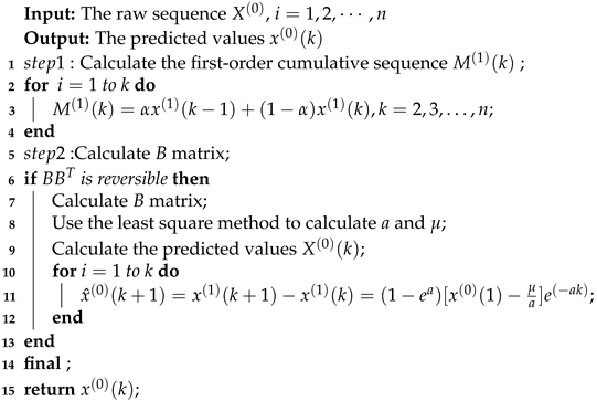2.2. Grey Model of Caputo Type Fractional Derivative

The fractional form of grey model was proposed by Liu et al. [15] in 2013. The goal of this model is to address several of the flaws in classic grey prediction models. For example, the existing GM(1,1) model cannot be utilized to accurately predict many real-world systems since the system behavior is influenced by other factors, and its eigenvalues do not fully obey the grey exponential law. To compare economic growth in Nigeria and Kenya, Awe et al. [16] use a fractional integration approach.

Let us take a quick look at the grey model’s fractional order accumulation.

Set nonnegative sequence $X^{\left(0\right)}=\left\{x^{\left(0\right)}\left(1\right),x^{\left(0\right)}\left(2\right),\dots ,x^{\left(0\right)}\left(n\right)\right\}$, the grey model of the $\alpha (0<\alpha <1)$ order equation with one variable GM($\alpha$, 1) is

$$\begin{array}{c}\hfill {\beta }^{\left(1\right)}{x}^{(1-\alpha )}\left(k\right)+a{m}^{\left(0\right)}\left(k\right)=\mu \end{array}$$

(8)

where $m^{\left(0\right)}\left(k\right)=\frac{x^{(1-\alpha )}\left(k\right)+x^{(1-\alpha )}(k-1)}{2}$, ${\beta }^{\left(1\right)}{x}^{(1-\alpha )}\left(k\right)$ represents the $1-\alpha$-order difference of $x^{\left(0\right)}\left(k\right)$. The least square estimation of GM($\alpha$, 1) model parameters satisfies

$$\left[\begin{array}{c}a\\ \mu \end{array}\right]={\left(B^{T}B\right)}^{-1}{B}^{T}Y,$$

where

$$B=\left[\begin{array}{cc}-m^{\left(0\right)}\left(2\right)& 1\\ -m^{\left(0\right)}\left(3\right)& 1\\ \dots & \dots \\ -m^{\left(0\right)}\left(n\right)& 1\end{array}\right],$$

and

$$Y=\left[\begin{array}{c}{\beta }^{\left(1\right)}{x}^{(1-\alpha )}\left(2\right)\\ {\beta }^{\left(1\right)}{x}^{(1-\alpha )}\left(3\right)\\ \dots \\ {\beta }^{\left(1\right)}{x}^{(1-\alpha )}\left(n\right)\end{array}\right].$$

The whitening equation of GM($\alpha$,1) model is

$$\begin{array}{c}\hfill \frac{d^{\alpha }{x}^0\left(t\right)}{d{t}^{\alpha }}+a{x}^{\left(0\right)}\left(t\right)=\mu .\end{array}$$

(9)

Let ${\widehat{x}}^{\left(0\right)}\left(1\right)=x^{\left(0\right)}\left(1\right)$, by fractional Laplace transform, the solution of Formula (9) is

$$\begin{array}{c}\hfill x^{\left(0\right)}\left(t\right)=(x^{\left(0\right)}\left(1\right)-\frac{\mu }{a})\sum _{k=0}^{\infty }\frac{{(-a{t}^{\alpha })}^k}{\Gamma (\alpha k+1)}+\frac{\mu }{a}.\end{array}$$

(10)

Thus the fitting value of GM($\alpha$,1) model is

$$\begin{array}{c}\hfill x^{\left(0\right)}\left(k\right)=(x^{\left(0\right)}\left(1\right)-\frac{\mu }{a})\sum _{k=0}^{\infty }\frac{{(-a{t}^{\alpha })}^i}{\Gamma (\alpha i+1)}+\frac{\mu }{a}.\end{array}$$

(11)

The pseudocode of GM($\alpha$,1) is given by Algorithm 2, as shown below:

Algorithm 2: GM($\alpha$,1) model.

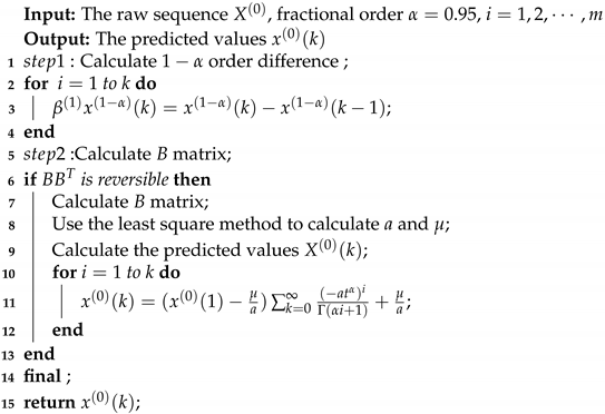2.3. Accuracy Testing of GM(1,1) and GM(0.95,1)

Extrapolating the projected value can be done using a model with excellent fitting accuracy. If this is not the case, residual correction must be performed first. To verify the accuracy of GM(1,1) and GM($\alpha$,1), the posterior error detection approach is usually utilized. The posterior error ration (C) and small error probability (P) are two fitting testing measures.

The ratio of residual standard deviation ($S_2$) to data standard deviation ($S_1$) is known as the posterior error ration (C). Obviously, the prediction accuracy improves as the residual standard deviation decreases. The following is the exact formula:

$$\begin{array}{c}\hfill C=\frac{S_2}{S_1}.\end{array}$$

(12)

In the Formula (12),

$$\begin{array}{c}\hfill S_1^2=\frac{1}{n}\sum _{i=1}^n{(X_{\left(i\right)}^{\left(0\right)}-\overline{X})}^2,\end{array}$$

and

$$\begin{array}{c}\hfill S_2^2=\frac{1}{n}\sum _{i=1}^n{({\epsilon }_{\left(i\right)}-\overline{\epsilon })}^2.\end{array}$$

The small error probability is shown in (13), for a given $P_0$, when $P<P_0$, the model is called a qualified model with small error probability:

$$\begin{array}{c}\hfill P=P\left(\right|{\epsilon }_{\left(i\right)}-\overline{\epsilon }|<0.6745S_1).\end{array}$$

(13)

According to the above two indicators, the forecast level is divided into four levels (see Table 1).

Table 1. Accuracy grade reference table.

Accuracy Class	Index Critical Value
	P	C
First-level	$P\ge 0.95$	$C\le 0.35$
Second-level	$0.80\le P<0.95$	$0.35<C\le 0.50$
Third-level	$0.70\le P<0.80$	$0.50<C\le 0.65$
Forth-level	$P<0.70$	$C>0.65$

To make it easier to compare GDP between years, the GDP used here was transformed into an unchangeable local currency. The training sample consisted of data from 1973 to 2011, whereas the test sample consisted of data from 2012 to 2016. Furthermore, we evaluated the model using the average absolute deviation (MAD) and the coefficient of determination ($R^2$), and we compared the model’s prediction effect using the absolute error criterion. Keep the following definitions in mind:

$$\begin{array}{c}\hfill \mathrm{MAD}=\frac{{\displaystyle \sum _{i=1}^n}|X_i-\widehat{X_i}|}{n},\end{array}$$

(14)

and

$$\begin{array}{c}\hfill AR{E}_i=\left|\frac{X_i-\widehat{X_i}}{X_i}\right|,i=1,2,\dots ,n,\end{array}$$

(15)

and

$$\begin{array}{c}\hfill R^2=1-\frac{{\displaystyle \sum _{i=1}^n}{(X_i-\widehat{X_i})}^2}{{\displaystyle \sum _{i=1}^n}{(X_i-\overline{X})}^2}.\end{array}$$

(16)

To compare the quality of models, we commonly utilize the Akaike information criterion (AIC) and Bayesian information criterion (BIC). The better the model, the lower the AIC and BIC values. AIC criterion has an overfitting problem when compared to BIC criterion. As a result, we use the following BIC standards:

$$\begin{array}{c}\hfill \mathrm{BIC}=log\left(\frac{1}{n}\sum _{i=1}^n{(X_i-{\widehat{X}}_i)}^2\right)+\frac{plogn}{n}.\end{array}$$

(17)

3. Main Results

The data in this section comes from the World Bank’s records from 1973 to 2016. Calculate the MAD, $R^2$, and BIC index values in the training sample set (see Table 2).

Table 2. Different values of grey model.

	GM(1,1)			GM(0.95,1)
	MAD	${\mathit{R}}^2$	BIC	MAD	${\mathit{R}}^2$	BIC
CAN	34414448765	0.9879086	48.94679	33734534311	0.9895514	48.80076
FRA	68364065162	0.9728951	50.37659	57357310718	0.9803684	50.05402
DEU	99453931115	0.9693005	50.94267	81811419026	0.9785968	50.58196
ITA	117484780283	0.8545935	51.33698	103872866630	0.8876252	51.07928
JPN	393677491323	0.8690739	53.69981	358667602223	0.8947864	53.48117
GBR	68468956596	0.9761038	50.34167	63648656598	0.9790246	50.2113
USA	467398760671	0.9766464	54.18997	420061610319	0.9809567	53.98594
EUU	441146078640	0.974133	54.12246	375276253076	0.9795674	53.88662

As can be seen from Table 2, the $MAD$ value and $BIC$ value of fractional grey prediction models in various countries are smaller than those of traditional grey prediction models, and $R^2$ is closer to 1, so the fitting effect is better.

Table 3 indicates that the grade of prediction accuracy is first-level for all posterior error ratios $C\le 0.35$ and tiny error probabilities $P\ge 0.95$. As a result, the constructed model can be utilized to forecast in the medium and long future.

Table 3. Accuracy testing values.

	GM(1,1)		GM(0.95,1)
	P	C	P	C
CAN	1	0.1158	1	0.1097
FRA	1	0.1644	1	0.1401
DEU	1	0.1750	1	0.1462
ITA	0.9318	0.3811	1	0.3352
JPN	1	0.3601	1	0.3240
GBR	1	0.1543	1	0.1448
USA	1	0.1516	1	0.1374
EUU	1	0.1605	1	0.1429

3.1. Fitting Result

To make it easier to compare the GM(1,1) and GM(0.95,1) models, the prediction results of the two models, as well as the original data, are presented as a line graph using Python and MATLAB, respectively, as shown in Figure 1. The trends and errors between them can be readily noticed using the graphical comparison.

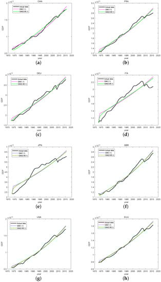
Figure 1. Fitting results for grey forecasting model for the G7 countries: (a) Canada (b), France (c), Germany (d), Italy (e), Japan (f), the United Kingdom (g), the United States (h), European Union.

It can be seen from Figure 1 that the fractional grey prediction model accurately shows the fluctuation law of data, and the error is small, while the fitting effect of the traditional grey prediction model is poor.

3.2. Predicted Results

The test data in this study is for GDP statistics from G7 countries from 2012 to 2016. The errors of the two prediction models are calculated and the errors are calculated using the absolute error as the error evaluation method. Table 4 shows the error pair of the prediction model in a summary comparison. The GM(0.95,1) model has a substantially lower prediction error for the data, as can be observed.

Table 4. Grey prediction model for G7 countries GDP data from 2012–2016.

	Year	Real Value	GM(1,1)	${\mathit{ARE}}_{\mathit{i}}$	GM(0.95,1)	${\mathit{ARE}}_{\mathit{i}}$
	2012	1693194096275.46	1725185175714.73	0.018896388	1698914426493.6	0.013003404
	2013	1735100681636.87	1768329586608.14	0.019151396	1730008754583.54	0.01207392
CAN	2014	1779611206826.42	1812552977438.03	0.018511347	1761154346219.05	0.010233611
	2015	1796369375909.66	1857882331947.61	0.034242574	1792351828024.82	0.024592371
	2016	1822735534879.33	1904345308704.84	0.04477068	1823601834354.28	0.033744816
	2012	2706807051174.77	2783679136379.47	0.027187873	2763087648243.83	0.019589538
	2013	2722404797996.28	2836504877221.62	0.042832675	2811708863760.12	0.033716494
FRA	2014	2748201937555.55	2890333089526.44	0.051030214	2861110591403.97	0.040403851
	2015	2777537939261.97	2945182797145.19	0.059418272	2911308024499.58	0.047233102
	2016	2810525379194.34	3001073384943.69	0.067997646	2962316477892.66	0.054205152
	2012	3559587403262.56	3646203072205.31	0.024214346	3620958453453.06	0.017123161
	2013	3577014590829.77	3710799857365.53	0.036536273	3680165471151.48	0.027979182
DEU	2014	3646039898346.43	3776541050714.31	0.034668781	3740240804303.89	0.024723508
	2015	3709597862509.39	3843446926791.69	0.035969522	3801200755783.78	0.024582414
	2016	3781698549834.74	3911538119324.91	0.034798444	3863061697944.44	0.021973994
	2012	2077060704620.29	2226728267130.19	0.070542436	2203799127286.2	0.059518811
	2013	2041165755679.07	2257377439911.16	0.106557569	2230621869130.45	0.093442093
ITA	2014	2043486014884.01	2288448474580.78	0.121788468	2257706880792.64	0.106719059
	2015	2063873410309.19	2319947177737.88	0.12618795	2285059098433.64	0.10925199
	2016	2083322583449.54	2351879435904.69	0.130711267	2312683379473.8	0.111867009
	2012	5778636370123.56	6186003375607.0	0.070242799	6126496812980.12	0.059947545
	2013	5894237388118.86	6300780322154.25	0.06974199	6231076789596.91	0.057907774
JPN	2014	5914022267462.79	6417686874306.06	0.085903024	6337272922468.91	0.072296603
	2015	5986140110537.86	6536762545398.38	0.091279223	6445116233574.44	0.075979338
	2016	6047894004051.61	6658047581909.06	0.100503733	6554637940727.12	0.08341123
	2012	2513321589693.39	2627121154069.95	0.046661814	2610421183989.1	0.04000844
	2013	2564904713179.98	2686476667723.88	0.049404948	2666139239003.77	0.04146064
GBR	2014	2643243341332.76	2747173222309.94	0.040595918	2722980002145.48	0.031431819
	2015	2705252231411.39	2809241116458.62	0.036620338	2780968390027.45	0.026187598
	2016	2753793133582.5	2872711333348.69	0.044622303	2840129727689.47	0.032774446
	2012	15542161722300	16194007236103.12	0.04477466	16081562735296.5	0.037520176
	2013	15802855301300	16628304384219.62	0.052424328	16493206997255.5	0.043873861
USA	2014	16208861247400	17074248681192.62	0.053965968	16915003030371.25	0.04413599
	2015	16672691917800	17532152484764.25	0.04982949	17347214175968.12	0.03875534
	2016	16920327941800	18002336529606.62	0.065227014	17790109806427.38	0.052669219
	2012	17206500000000	17871609712710.75	0.039047076	17744873110260.31	0.031678669
	2013	17251100000000	18232171082420.25	0.053882722	18079082959715.0	0.045033697
EUU	2014	17551100000000	18600006810926.25	0.056818569	18419114699868.69	0.046540608
	2015	17957000000000	18975263659086.88	0.054181314	18765086361202.56	0.042504798
	2016	18305200000000	19358091348673.75	0.057819199	19117117295279.62	0.044651218

4. Conclusions

Because most systems in real life are fractional order, in order to improve the accuracy and application scope of grey prediction, this paper uses fractional order accumulation to replace the traditional grey index effect, and then gives the pseudo codes of the two models, which are applied to the economic growth prediction of the Group of Seven. The results show that, compared with the classical grey prediction model, the fractional prediction model has better prediction effect in medium and long-term prediction. Finally, we give the GDP forecast of G7 countries from 2012 to 2016, and compare it with the actual data to further prove the prediction effect of the fractional grey prediction model.

References

- Deng, J. Control problems of grey systems. Syst. Control. Lett. 1982, 1, 288–294. [Google Scholar]
- Deng, J. Essential Topics on Grey Systems: Theory and Applications; China Ocean Press: Beijing, China, 1988. [Google Scholar]
- Tien, T. A research on the grey prediction model GM(1,n). Appl. Math. Comput. 2012, 218, 4903–4916. [Google Scholar] [CrossRef]
- Li, D.; Chang, C.; Chen, C.; Kilicman, A. Forecasting short-term electricity consumption using the adaptive grey-based approach-An Asian case. Omega 2012, 40, 767–773. [Google Scholar] [CrossRef]
- Zhu, Z.; Cao, H. A fractional calculus based model for the simulation of an outbreak of dengue fever. J. Trop. Meteorol. 1998, 4, 359–365. [Google Scholar]
- Tien, T. The indirect measurement of tensile strength of material by the grey prediction model GMC(1, n). Meas. Sci. Technol. 2005, 16, 1322–1328. [Google Scholar] [CrossRef]
- Chen, C.; Tien, T. A new forecasting method for time continuous model of dynamic system. Appl. Math. Comput. 1996, 80, 225–244. [Google Scholar] [CrossRef]
- Chen, C.; Tien, T. A new transfer function model: The grey dynamic model GDM(2,2,1). Int. J. Syst. Sci. 1996, 27, 1371–1379. [Google Scholar] [CrossRef]
- Chen, C.; Tien, T. The indirect measurement of tensile strength by the deterministic grey dynamic model DGDM(1,1,1). Int. J. Syst. Sci. 1997, 28, 683–690. [Google Scholar] [CrossRef]
- Chen, C.; Tien, T. A new forecasting method of discrete dynamic system. Appl. Math. Comput. 1997, 86, 61–84. [Google Scholar] [CrossRef]
- Tien, T. A research on the prediction of machining accuracy by the deterministic grey dynamic model DGDM (1,1,1). Appl. Math. Comput. 2005, 161, 923–945. [Google Scholar] [CrossRef]
- Tien, T. The deterministic grey dynamic model with convolution integral DGDMC(1,n). Appl. Math. Model. 2009, 33, 3498–3510. [Google Scholar] [CrossRef] [Green Version]
- Tien, T. The indirect measurement of tensile strength for a higher temperature by the new model IGDMC(1,n). Measurement 2008, 41, 662–675. [Google Scholar] [CrossRef]
- Tien, T.; Chen, C. Forecasting CO2 output from gas furnace by a new transfer function model GDM(2,2,1). Syst. Anal. Model. Simul. 1998, 30, 265–287. [Google Scholar]
- Wu, L.; Liu, S.; Yao, L.; Yan, S.; Liu, D. Grey system model with the fractional order accumulation. Commun. Nonlinear Sci. Numer. Simul. 2013, 18, 1775–1785. [Google Scholar] [CrossRef]
- Awe, O.O.; Mudida, R.; Gil-Alana, L.A. Comparative analysis of economic growth in Nigeria and Kenya: A fractional integration approach. Int. J. Financ. Econ. 2021, 26, 1197–1205. [Google Scholar] [CrossRef]
Publisher’s Note: MDPI stays neutral with regard to jurisdictional claims in published maps and institutional affiliations. |
© 2022 by the authors. Licensee MDPI, Basel, Switzerland. This article is an open access article distributed under the terms and conditions of the Creative Commons Attribution (CC BY) license (https://creativecommons.org/licenses/by/4.0/).