Deterministic and Stochastic Prey–Predator Model for Three Predators and a Single Prey

Abstract

In this paper, a deterministic prey–predator model is proposed and analyzed. The interaction between three predators and a single prey was investigated. The impact of harvesting on the three predators was studied, and we concluded that the dynamics of the population can be controlled by harvesting. Some sufficient conditions were obtained to ensure the local and global stability of equilibrium points. The transcritical bifurcation was investigated using Sotomayor’s theorem. We performed a stochastic extension of the deterministic model to study the fluctuation environmental factors. The existence of a unique global positive solution for the stochastic model was investigated. The exponential–mean–squared stability of the resulting stochastic differential equation model was examined, and it was found to be dependent on the harvesting effort. Theoretical results are illustrated using numerical simulations.

1. Introduction

Lotka and Volterra independently created two types of prey–predatory models known as the “Lotka–Volterra model” [1,2]. Since then, many scientists have modified and developed the Lotka–Volterra model to accurately describe the ecosystem. Numerous studies have examined the case of the presence of more than one predator [2,3,4,5,6,7,8,9,10,11]. Mukhopadhyay and Bhattacharyya [12] formulated a mathematical model of two predators living on a single biotic prey. They assumed that the predation function for the first predator follows the mass action kinetics, while the functional response for the second predator obeys the Holling type–II functional response. They also assumed that one of the predators is economically viable and undergoes harvesting at a rate proportional to its density. According to [13], in the northern Alaskan forest community, moose are the only large herbivores, constituting the primary prey for each of the three predators: black bears, gray wolves, and brown bears. Black bears have been known to attack and consume wolves if the opportunity presents itself. The main feature of this paper was to modify the interference of the predators in the system investigated in [12] by adding an extra predator $y\left(t\right)$ where the first predator (black bear) preys on the second predator (gray wolves) in addition to the prey. The focus was on the harvesting rates and carrying capacity parameters of the model. The paper is organized as follows: The mathematical model is given in Section 2. The existence, uniqueness, non–negativity, and boundedness of the system are all verified in Section 3. Section 4 investigates the local and global stability of the system’s equilibrium points. The stochastic extension of the deterministic model is conducted in Section 5. The numerical simulations presented in Section 6 are used to verify the theoretical results. Finally, in Section 7, the conclusions are presented.

2. Mathematical Model

In this paper, we considered a four–species prey–predator model with one prey and three predators as follows:

$$\begin{array}{c}\hfill \begin{array}{cc}\hfill \frac{dx}{dt}& =rx(1-\frac{x}{k})-{\beta }_{1}xy-{\beta }_{2}xz-\frac{{\beta }_{3}xw}{a+x},\hfill \\ \hfill \frac{dy}{dt}& =m_{1}xy+\delta yz-{\mu }_{1}y-q_{1}Ey,\hfill \\ \hfill \frac{dz}{dt}& =m_{2}xz-\delta yz-{\mu }_{2}z-q_{2}Ez,\hfill \\ \hfill \frac{dw}{dt}& =\frac{m_{3}xw}{a+x}-{\mu }_{3}w-q_{3}Ew,\hfill \end{array}\end{array}$$

(1)

where $x\left(t\right)$ is the population size of the single prey species. We assumed that $x\left(t\right)$ grows logistically in the absence of predators with intrinsic growth rate r and carrying capacity k. The first predator $y\left(t\right)$ has the ability to consume both the prey and second predator $z\left(t\right)$ with the Holling type I (linear) functional response. Let the interaction between the third predator $w\left(t\right)$ and prey follow the Holling type II functional response. Assume ${\beta }_i(i=1,2,3)$ denote the predation rates of the first, second, and third predators on the prey, respectively, and a is the half–saturation constant. Furthermore, let $m_i(i=1,2,3)$ denote the efficiency of the first, second, and third predators in the presence of the prey. Moreover, $\delta$ represents the predation rate of the first predator on the second predator. We assumed that the ecological efficiency of the second predator’s biomass z in the first predator’s biomass y is unity. We also assumed that the predators economically undergo harvesting at a rate proportional to their density. The constants $q_i(i=1,2,3)$ denote the catchability constants, while E represents the harvesting effort. The density of the first, second, and third predator populations decreases due to natural death at constant rates ${\mu }_1$, ${\mu }_2$, and ${\mu }_3$, respectively.

3. Some Preliminary Results

3.1. Existence and Uniqueness

In this section, we investigate the existence and uniqueness of the solutions of the prey–predator system (1) in the region ${\mathrm{\Theta }}_1\times \left(0,T\right]$ where:

$${\mathrm{\Theta }}_1=\left\{(x,y,z,w)\in {\mathbb{R}}_{+}^4:max\left(\left|x\right|,\left|y\right|,\left|z\right|,\left|w\right|\right)\le \phi \right\},$$

for sufficiently large $\phi$.

Theorem 1.

For each $X_0=(x_0,y_0,z_0,w_0)\in {\mathrm{\Theta }}_1$, there exists a unique solution $X\left(t\right)\in {\mathrm{\Theta }}_1$ of the prey–predator system (1), which is defined for all $t\ge 0$.

Proof. 

Define a mapping $F\left(X\right)=(F_1\left(X\right),F_2\left(X\right),F_3\left(X\right),F_4\left(X\right))$, in which:

$$\begin{array}{c}\hfill \begin{array}{cc}\hfill F_1\left(X\right)& =rx(1-\frac{x}{k})-{\beta }_{1}xy-{\beta }_{2}xz-\frac{{\beta }_{3}xw}{a+x},\hfill \\ \hfill F_2\left(X\right)& =m_{1}xy+\delta yz-({\mu }_1+q_{1}E)y,\hfill \\ \hfill F_3\left(X\right)& =m_{2}xz-\delta yz-({\mu }_2+q_{2}E)z,\hfill \\ \hfill F_4\left(X\right)& =\frac{m_{3}xw}{a+x}-({\mu }_3+q_{3}E)w.\hfill \end{array}\end{array}$$

(2)

For any $X,\overline{X}\in {\mathrm{\Theta }}_1,$ it follows from (1) that:

$$\begin{array}{cc}\hfill ∥F\left(X\right)-F\left(\overline{X}\right)∥=& \left|F_1\left(X\right)-F_1\left(\overline{X}\right)\right|+\left|F_2\left(X\right)-F_2\left(\overline{X}\right)\right|+\left|F_3\left(X\right)-F_3\left(\overline{X}\right)\right|+\left|F_4\left(X\right)-F_4\left(\overline{X}\right)\right|\hfill \\ \hfill =& \left|rx(1-\frac{x}{k})-{\beta }_{1}xy-{\beta }_{2}xz-\frac{{\beta }_{3}xw}{a+x}-r\overline{x}(1-\frac{\overline{x}}{k})+{\beta }_1\overline{x}\overline{y}+{\beta }_2\overline{x}\overline{z}+\frac{{\beta }_3\overline{x}\overline{w}}{a+\overline{x}}\right|\hfill \\ \hfill & +\left|m_{1}xy+\delta yz-({\mu }_1+q_{1}E)y-m_1\overline{x}\overline{y}-\delta \overline{y}\overline{z}+({\mu }_1+q_{1}E)\overline{y}\right|\hfill \\ \hfill & +\left|m_{2}xz-\delta yz-({\mu }_2+q_{2}E)z-m_2\overline{x}\overline{z}+\delta \overline{y}\overline{z}+({\mu }_2+q_{2}E)\overline{z}\right|\hfill \\ & +\left|\frac{m_{3}xw}{a+x}-({\mu }_3+q_{3}E)w-\frac{m_3\overline{x}\overline{w}}{a+\overline{x}}+({\mu }_3+q_{3}E)\overline{w}\right|\hfill \\ \hfill \le & \left(r+\frac{2\phi r}{k}+\frac{2\phi }{a}+{\rho }_1\phi \right)|x-\overline{x}|+\left(({\mu }_1+q_{1}E)(\phi +1)+({\beta }_1+2\delta )\phi \right)|y-\overline{y}|\hfill \\ \hfill & +\left(m_2\phi +{\beta }_2\phi +2\delta \phi +{\mu }_2+q_{2}E\right)|z-\overline{z}|+\left(\frac{2\phi }{a}+\frac{2{\phi }^2}{a^2}+{\mu }_3+q_{3}E\right)|w-\overline{w}|\hfill \\ \hfill \le & H_0∥X-\overline{X}∥,\hfill \end{array}$$

where:

$$H_0=max\left\{r+\frac{2\phi r}{k}+\frac{2\phi }{a}+{\rho }_1\phi ,{\rho }_2\phi +({\mu }_1+q_{1}E),{\rho }_3\phi +({\mu }_2+q_{2}E),\frac{2\phi }{a}+\frac{2{\phi }^2}{a^2}+({\mu }_3+q_{3}E)\right\},$$

where ${\rho }_1=({\beta }_1+{\beta }_2+m_1+m_2)$, ${\rho }_2=(m_1+q_{1}E+{\beta }_1+2\delta )$, and ${\rho }_3=(m_2+{\beta }_2+2\delta )$. Hence, $F\left(X\right)$ satisfies the Lipschitz condition with respect to X. According to [14], as $F\left(X\right)$ is locally Lipschitz, then there exists a unique local solution to the three–predator–one–prey system (1). □

3.2. Non-Negativity and Boundedness

Considering the biological significance of the problem, we were only interested in non–negative and bounded solutions. The prey–predator system (1) can be written as follows:

$$\begin{array}{c}\hfill \begin{array}{cc}\hfill x\left(t\right)& =x\left(0\right)e^{{\int }_0^t\frac{F_1\left(X\left(s\right)\right)}{x}ds}\ge 0,\hfill \\ \hfill y\left(t\right)& =y\left(0\right)e^{{\int }_0^t\frac{F_2\left(X\left(s\right)\right)}{y}ds}\ge 0,\hfill \\ \hfill z\left(t\right)& =z\left(0\right)e^{{\int }_0^t\frac{F_3\left(X\left(s\right)\right)}{z}ds}\ge 0,\hfill \\ \hfill w\left(t\right)& =w\left(0\right)e^{{\int }_0^t\frac{F_4\left(X\left(s\right)\right)}{w}ds}\ge 0,\hfill \end{array}\end{array}$$

(3)

with initial values $x\left(0\right)=x_0\ge 0,y\left(0\right)=y_0\ge 0,z\left(0\right)=z_0\ge 0,w\left(0\right)=w_0\ge 0$. Thus, the solution of the model (1), with non–negative initial conditions remains non–negative. Furthermore, the solution satisfies the Lipschitz condition, as stated in Theorem 1. By Theorems 5 and 6 in [14], the solution of the prey–predator model (1) satisfies the non–negativity. The boundedness of the solutions of model (1) is given in the following theorem.

Theorem 2.

The solutions of the prey–predator model (1) starting in ${\mathbb{R}}_{+}^4$ are uniformly bounded.

Proof. 

Let $\left(x\right(t),y(t),z(t),w(t\left)\right)$ be any solution of the system (1) with non–negative initial conditions. Let $H_1\left(t\right)=x\left(t\right)+y\left(t\right)+z\left(t\right)+w\left(t\right),$ then:

$$\begin{array}{c}\hfill \begin{array}{cc}\hfill \frac{d{H}_1}{dt}+\mu H_1& \le rx\left(1-\frac{x}{k}\right)+\mu x\hfill \\ \hfill & \le -\frac{r}{k}{\left(x-\frac{k(r+\mu )}{2r}\right)}^2+\frac{k{(r+\mu )}^2}{4r},\hfill \end{array}\end{array}$$

where $\mu =\min \left\{{\mu }_1,{\mu }_2,{\mu }_3\right\}$, thus:

$$0\le H_1\left(t\right)\le \frac{k{(r+\mu )}^2}{4\mu r},\mathrm{as}t\to \infty .$$

As a result, all the solutions of the prey–predator model (1) that start in ${\mathbb{R}}_{+}^4$ are uniformly bounded in the region:

$${\mathrm{\Theta }}_2=\left\{(x,y,z,w)\in {\mathbb{R}}_{+}^4:H_1\left(t\right)\le \frac{k{(r+\mu )}^2}{4\mu r}+\xi ,\mathrm{for}\mathrm{any}\xi >0\right\}.$$

□

In the following, three critical parameters $R_1$, $R_2$, and $R_3$, can be used to classify the dynamics of the prey–predator model (1). The threshold parameter $R_1$ is defined by $R_1=\frac{m_{1}k}{({\mu }_1+q_{1}E)},$ while the threshold parameter $R_2$ is defined by $R_2=\frac{m_{2}k}{({\mu }_2+q_{2}E)}.$ The threshold parameter $R_3$ is defined by $R_3=\frac{m_{3}k}{({\mu }_3+q_{3}E)(a+k)}$. Using the next–generation method, one can obtain the basic reproduction number:

$$R_0=\max \left\{\frac{m_{1}k}{({\mu }_1+q_{1}E)},\frac{m_{2}k}{({\mu }_2+q_{2}E)},\frac{m_{3}k}{({\mu }_3+q_{3}E)(a+k)}\right\}.$$

One can note that the threshold parameter $R_1$ appears as a result of additional predator $y\left(t\right)$ in the system considered in [12].

4. Equilibria and Stability

The prey–predator model (1) has the following seven equilibrium points:

• The trivial equilibrium point $E_0=(0,0,0,0)$, which always exists;
• The predator free equilibrium point $E_1=\left(k,0,0,0\right)$, which always exists;
• The equilibrium point $E_2=(\frac{({\mu }_1+q_{1}E)}{m_1},\frac{r({\mu }_1+q_{1}E)(R_1-1)}{m_1{\beta }_{1}k},0,0);$$E_2$ exists if $R_1>1;$
• The equilibrium point $E_3=(\frac{({\mu }_2+q_{2}E)}{m_2},0,\frac{r({\mu }_2+q_{2}E)(R_2-1)}{m_2{\beta }_{2}k},0);$$E_3$ exists if $R_2>1;$
• The equilibrium point $E_4=(\frac{a({\mu }_3+q_{3}E)}{m_3-({\mu }_3+q_{3}E)},0,0,\frac{ar{m}_3({\mu }_3+q_{3}E)(a+k)(R_3-1)}{k{\beta }_3{(m_3-({\mu }_3+q_{3}E))}^2});$$E_4$ exists if $R_3>1$;
• The equilibrium point $E_5=(x_5,y_5,z_5,0)$, where:

  $$x_5=\frac{k\left(\delta r+{\beta }_1({\mu }_2+q_{2}E)-{\beta }_2({\mu }_1+q_{1}E)\right)}{\varphi },y_5=\frac{m_2{x}_5-({\mu }_2+q_{2}E)}{\delta },z_5=\frac{({\mu }_1+q_{1}E)-m_1{x}_5}{\delta },$$

  where $\varphi =\delta r+{\beta }_1{m}_{2}k-{\beta }_2{m}_{1}k$. $E_5$ exists if $\frac{({\mu }_2+q_{2}E)}{m_2}<x_5<\frac{({\mu }_1+q_{1}E)}{m_1};$
• The coexistence equilibrium point $E_6=(x_6,y_6,z_6,w_6)$, where:

  $$x_6=\frac{a({\mu }_3+q_{3}E)}{m_3-({\mu }_3+q_{3}E)},y_6=\frac{m_2{x}_6-({\mu }_2+q_{2}E)}{\delta },z_6=\frac{({\mu }_1+q_{1}E)-m_1{x}_6}{\delta },$$

  $$w_6=\frac{(a+x_6)}{k{\beta }_3}\left[r(k-x_6)-k{\beta }_1{y}_6-k{\beta }_2{z}_6\right].$$
  $E_6$ exists if $m_3>{\mu }_3+q_{3}E$, $r{x}_6+k{\beta }_1{y}_6+k{\beta }_2{z}_6<rk$ and $\frac{({\mu }_2+q_{2}E)}{m_2}<x_6<\frac{({\mu }_1+q_{1}E)}{m_1}$.

One can note that the additional predator $y\left(t\right)$ causes two new equilibrium points $E_2$ and $E_5$ to be obtained, which were not present in [12]. Now, the local stability of the system (1) is investigated. The Jacobian matrix is given as follows:

$$J=\left(\begin{array}{cccc}r\left(1-\frac{2x}{k}\right)-{\beta }_{1}y-{\beta }_{2}z-\frac{a{\beta }_{3}w}{{(a+x)}^2}& -{\beta }_{1}x& -{\beta }_{2}x& -\frac{{\beta }_{3}x}{a+x}\\ m_{1}y& m_{1}x+\delta z-({\mu }_1+q_{1}E)& \delta y& 0\\ m_{2}z& -\delta z& m_{2}x-\delta y-({\mu }_2+q_{2}E)& 0\\ \frac{a{m}_{3}w}{{(a+x)}^2}& 0& 0& \frac{m_{3}x}{a+x}-({\mu }_3+q_{3}E)\end{array}\right).$$

The eigenvalues of J around the trivial point $E_0$ are $r,-({\mu }_1+q_{1}E),-({\mu }_2+q_{2}E)$ and $-({\mu }_3+q_{3}E)$; therefore, for all parameters, $E_0$ is a saddle with three–dimensional stable manifolds and a one–dimensional unstable manifold. The stability of the free predators’ equilibrium point $E_1=(k,0,0,0)$ is studied as follows:

Theorem 3.

If $R_0<1$, then $E_1$ is locally asymptotically stable.

Proof. 

The Jacobian matrix of the model (1) around $E_1\left(J\left(E_1\right)\right)$ is as follows:

$$J\left(E_1\right)=\left(\begin{array}{cccc}-r& -{\beta }_{1}k& -{\beta }_{2}k& -\frac{{\beta }_{3}k}{a+k}\\ 0& m_{1}k-({\mu }_1+q_{1}E)& 0& 0\\ 0& 0& m_{2}k-({\mu }_2+q_{2}E)& 0\\ 0& 0& 0& \frac{m_{3}k}{a+k}-({\mu }_3+q_{3}E)\end{array}\right).$$

(4)

The eigenvalues of $J\left(E_1\right)$ are $-r,m_{1}k-({\mu }_1+q_{1}E),m_{2}k-({\mu }_2+q_{2}E)$ and $\frac{m_{3}k}{a+k}-({\mu }_3+q_{3}E).$ Thus, $E_1$ is locally asymptotically stable if $R_0<1$. □

Theorem 4.

If $\frac{{\beta }_{1}k}{({\mu }_1+q_{1}E)}<1$, $\frac{{\beta }_{2}k}{({\mu }_2+q_{2}E)}<1$, and $\frac{m_{3}k}{({\mu }_3+q_{3}E)(a+k)}<1$, then $E_1$ is globally stable.

Proof. 

One can consider the positive–definite Lyapunov function as follows.

$$V_1=\left(x-k-kln\frac{x}{k}\right)+y+z+w.$$

By calculating the time derivative of $V_1$, one obtains:

$$\begin{array}{c}\hfill \begin{array}{cc}\hfill \frac{d{V}_1}{dt}\le & (x-k)\left(r(1-\frac{x}{k})-{\beta }_{1}y-{\beta }_{2}z-\frac{{\beta }_{3}w}{a+x}\right)+m_{1}xy+\delta yz-({\mu }_1+q_{1}E)y\hfill \\ \hfill +& m_{2}xz-\delta yz-({\mu }_2+q_{2}E)z+\frac{m_{3}xw}{a+x}-({\mu }_3+q_{3}E)w\hfill \\ \hfill \le & -\frac{r}{k}{(x-k)}^2+({\beta }_{1}k-({\mu }_1+q_{1}E))y+({\beta }_{2}k-({\mu }_2+q_{2}E))z+(\frac{m_{3}k}{a+k}-({\mu }_3+q_{3}E))w.\hfill \end{array}\end{array}$$

In accordance with Lyapunov–Sasalle’s invariance principle, $E_1$ is globally stable when $\frac{{\beta }_{1}k}{({\mu }_1+q_{1}E)}<1$, $\frac{{\beta }_{2}k}{({\mu }_2+q_{2}E)}<1$, and $\frac{m_{3}k}{({\mu }_3+q_{3}E)(a+k)}<1$. □

One can note that the global stability of $E_1$ depends on the parameters ${\beta }_1,{\mu }_1$ and $q_1$ of additional predator $y\left(t\right)$, which were not present in [12]. The local bifurcation near the equilibrium point $E_1$ of the system (1) is now investigated using Sotomayor’s theorem [15].

Theorem 5.

The prey–predator model (1) goes through a transcritical bifurcation regarding the bifurcation parameter $q_1$ around $E_1=(k,0,0,0)$ if $R_1=1$.

Proof. 

The Jacobian matrix of the prey–predator model (1) at $E_1$ with $q_1=q_1^{*}=\frac{{\mu }_{1}k-{\mu }_1}{E}$ has a zero eigenvalue. The eigenvector corresponding to $J\left(E_1\right)Q_1=0$ is $Q_1={({\nu }_1,-\frac{-r{\nu }_1}{{\beta }_{1}k},0,0)}^T$, where ${\nu }_1$ is any non-zero real number. Similarly, the eigenvector corresponding to $J{\left(E_1\right)}^T{Q}_2=0$ is given by $Q_2={\left(0,{\tau }_2,0,0\right)}^T,$ where ${\tau }_2$ is any non–zero number. Thus:

• $Q_2^T{F}_{m_1}(E_1,m_1^{*})=0$;
• $Q_2^{T}D{F}_{m_1}(E_1,m_1^{*})Q_1=\frac{-rE{\nu }_1{\tau }_2}{{\beta }_{1}k}\ne 0$;
• $Q_2^T{D}^{2}F(E_1,m_1^{*})(Q_1,Q_1)=2\left(m_1{\nu }_1+\delta {\nu }_3\right){\tau }_2{\nu }_2\ne 0.$

In accordance with Sotomayor’s theorem, the prey–predator model (1) has a transcritical bifurcation at $q_1^{*}$, which is equivalent to $R_1=1$. Therefore, the proof is complete. □

The stability around $E_2=(x_2,y_2,0,0)$ is studied as follows:

Theorem 6.

If $\frac{m_3{x}_2}{({\mu }_3+q_{3}E)(a+x_2)}<1$ and $\frac{m_2{x}_2}{({\mu }_2+q_{2}E)+\delta y_2}<1$, then $E_2$ is locally stable.

Proof. 

The eigenvalues of $J\left(E_2\right)$ are:

$$\begin{array}{c}\hfill \begin{array}{cc}\hfill {\lambda }_1& =\frac{m_3{x}_2}{a+x_2}-({\mu }_3+q_{3}E),\hfill \\ \hfill {\lambda }_2& =m_2{x}_2-({\mu }_2+q_{2}E)-\delta y_2,\hfill \\ \hfill {\lambda }_3& =\frac{-r{x}_2-\sqrt{r^2{x}_2^2-4k{m}_1{\beta }_1{x}_2{y}_2}}{2k},\hfill \\ \hfill {\lambda }_4& =\frac{-r{x}_2+\sqrt{r^2{x}_2^2-4k{m}_1{\beta }_1{x}_2{y}_2}}{2k}.\hfill \end{array}\end{array}$$

The eigenvalues ${\lambda }_3$ and ${\lambda }_4$ have negative real parts. Thus, if $\frac{m_3{x}_2}{({\mu }_3+q_{3}E)(a+x_2)}<1$ and $\frac{m_2{x}_2}{({\mu }_2+q_{2}E)+\delta y_2}<1$, then $E_2$ is locally stable.

□

Theorem 7.

If $\frac{m_3{x}_2}{a({\mu }_3+q_{3}E)}<1$ and $\frac{m_2{x}_2}{({\mu }_2+q_{2}E)+\delta y_2}<1$, then $E_2$ is globally stable.

Proof. 

One can consider the positive–definite Lyapunov function as follows:

$$V_2=\left(x-x_2-x_{2}ln\frac{x}{x_2}\right)+\frac{{\beta }_2}{m_2}\left(y-y_2-y_{2}ln\frac{y}{y_2}\right)+\frac{{\beta }_2}{m_2}z+\frac{{\beta }_3}{m_3}w.$$

By taking the time derivative of $V_2$, one obtains,

$$\begin{array}{c}\hfill \begin{array}{cc}\hfill \frac{d{V}_2}{dt}\le & (x-x_2)\left(r(1-\frac{x}{k})-{\beta }_{1}y-{\beta }_{2}z-\frac{{\beta }_{3}w}{a+x}\right)+\frac{{\beta }_2}{m_2}(y-y_2)\left(m_{1}x+\delta z-({\mu }_1+q_{1}E)\right)\hfill \\ \hfill +& \frac{{\beta }_2}{m_2}\left(m_{2}xz-\delta yz-({\mu }_2+q_{2}E)z\right)+\frac{{\beta }_3}{m_3}\left(\frac{m_{3}x}{a+x}-({\mu }_3+q_{3}E)\right)w\hfill \\ \hfill \le & -\frac{r}{k}{(x-x_2)}^2+{\beta }_2\left(x_2-\frac{\delta y_2}{m_2}-\frac{({\mu }_2+q_{2}E)}{m_2}\right)z+{\beta }_3\left(\frac{x_2}{a+x}-\frac{({\mu }_3+q_{3}E)}{m_3}\right)w.\hfill \end{array}\end{array}$$

Thus, $E_2$ is globally stable if $\frac{m_3{x}_2}{a({\mu }_3+q_{3}E)}<1$ and $\frac{m_2{x}_2}{({\mu }_2+q_{2}E)+\delta y_2}<1$. □

The stability of the equilibrium point $E_3=(x_3,0,z_3,0)$ is investigated as follows:

Theorem 8.

If $\frac{m_3{x}_3}{(a+x_3)({\mu }_3+q_{3}E)}<1$ and $\frac{m_1{x}_3+\delta z_3}{({\mu }_1+q_{1}E)}<1$, then $E_3$ is locally stable.

Proof. 

The eigenvalues of $J\left(E_3\right)$ are:

$$\begin{array}{c}\hfill \begin{array}{cc}\hfill {\lambda }_1& =\frac{m_3{x}_3}{a+x_3}-({\mu }_3+q_{3}E),\hfill \\ \hfill {\lambda }_2& =m_1{x}_3-({\mu }_1+q_{1}E)+\delta z_3,\hfill \\ \hfill {\lambda }_3& =\frac{-r{x}_3-\sqrt{r^2{x}_3^2-4k{m}_3{\beta }_2{x}_3{z}_3}}{2k},\hfill \\ \hfill {\lambda }_4& =\frac{-r{x}_3+\sqrt{r^2{x}_3^2-4k{m}_3{\beta }_2{x}_3{z}_3}}{2k}.\hfill \end{array}\end{array}$$

The eigenvalues ${\lambda }_3$ and ${\lambda }_4$ have negative real parts. Thus, if $\frac{m_3{x}_3}{(a+x_3)({\mu }_3+q_{3}E)}<1$ and $\frac{m_1{x}_3+\delta z_3}{({\mu }_1+q_{1}E)}<1$, then the equilibrium point $E_3$ is locally stable. □

Theorem 9.

If $\frac{m_3{x}_3}{a({\mu }_3+q_{3}E)}<1$ and $\frac{m_1{x}_3+\delta z_3}{({\mu }_1+q_{1}E)}<1,$ then $E_3$ is globally stable.

Proof. 

One can consider the positive–definite Lyapunov function as follows:

$$V_3=\left(x-x_3-x_{3}ln\frac{x}{x_3}\right)+\frac{{\beta }_1}{m_1}y+\frac{{\beta }_1}{m_1}\left(z-z_3-z_{3}ln\frac{z}{z_3}\right)+\frac{{\beta }_3}{m_3}w.$$

By taking the time derivative of $V_3$, one obtains,

$$\begin{array}{c}\hfill \begin{array}{cc}\hfill \frac{d{V}_3}{dt}\le & (x-x_3)\left(r(1-\frac{x}{k})-{\beta }_{1}y-{\beta }_{2}z-\frac{{\beta }_{3}w}{a+x}\right)+\frac{{\beta }_1}{m_1}\left(m_{1}xy+\delta yz-({\mu }_1+q_{1}E)y\right)\hfill \\ \hfill +& \frac{{\beta }_1}{m_1}(z-z_3)\left(m_{2}x-\delta y-({\mu }_2+q_{2}E)\right)+\frac{{\beta }_{3}w}{m_3}\left(\frac{m_{3}x}{a+x}-({\mu }_3+q_{3}E)\right)\hfill \\ \hfill \le & -\frac{r}{k}{(x-x_3)}^2+\frac{{\beta }_1}{m_1}\left(m_1{x}_3+\delta z_3-({\mu }_1+q_{1}E)\right)y+{\beta }_3\left(\frac{x_3}{a+x}-\frac{({\mu }_3+q_{3}E)}{m_3}\right)w.\hfill \end{array}\end{array}$$

Thus, $E_3$ is globally stable if $\frac{m_3{x}_3}{a({\mu }_3+q_{3}E)}<1$ and $\frac{m_1{x}_3+\delta z_3}{({\mu }_1+q_{1}E)}<1$. □

The stability of the equilibrium point $E_4=(x_4,0,0,w_4)$ is studied as follows:

Theorem 10.

If $m_1{x}_4<{\mu }_1+q_{1}E$, $m_2{x}_4<{\mu }_2+q_{2}E$ and $1<R_3<1+\frac{a{m}_3}{({\mu }_3+q_{3}E)(a+k)}$, then $E_4$ is locally stable.

Proof. 

The eigenvalues of $J\left(E_4\right)$ are:

$$\begin{array}{c}\hfill \begin{array}{cc}\hfill {\lambda }_1& =m_1{x}_4-({\mu }_1+q_{1}E),\hfill \\ \hfill {\lambda }_2& =m_2{x}_4-({\mu }_2+q_{2}E),\hfill \end{array}\end{array}$$

The other eigenvalues are determined by:

$${\lambda }^2+x_4\left(\frac{r}{k}-\frac{{\beta }_3{w}_4}{{(a+x_4)}^2}\right)\lambda +\frac{a{m}_3{\beta }_3{x}_4{w}_4}{{(a+x_4)}^3}=0.$$

One can note that $\frac{r}{k}-\frac{{\beta }_3{w}_4}{{(a+x_4)}^2}>0$ is equivalent to $R_3<1+\frac{a{m}_3}{({\mu }_3+q_{3}E)(a+k)}$. Thus, if $m_1{x}_4<{\mu }_1+q_{1}E$, $m_2{x}_4<{\mu }_2+q_{2}E$, and $1<R_3<1+\frac{a{m}_3}{({\mu }_3+q_{3}E)(a+k)}$, then $E_4$ is locally stable.

□

The stability around $E_5=(x_5,y_5,z_5,0)$ is studied as follows:

Theorem 11.

If $\frac{m_3{x}_5}{({\mu }_3+q_{3}E)(a+x_5)}<1$, then $E_5$ is locally stable.

Proof. 

$J\left(E_5\right)$ is:

$$J\left(E_5\right)=\left(\begin{array}{cccc}-\frac{r{x}_5}{k}& -{\beta }_1{x}_5& -{\beta }_2{x}_5& -\frac{{\beta }_3{x}_5}{a+x_5}\\ m_1{y}_5& 0& \delta y_5& 0\\ m_2{z}_5& -\delta z_5& 0& 0\\ 0& 0& 0& \frac{m_3{x}_5}{a+x_5}-({\mu }_3+q_{3}E)\end{array}\right).$$

The first eigenvalue of $J\left(E_5\right)$ is ${\lambda }_1=\frac{m_3{x}_5}{a+x_5}-({\mu }_3+q_{3}E)$. The other roots are determined by

$${\lambda }^3+c_1{\lambda }^3+c_2\lambda +c_3=0,$$

where:

$$\begin{array}{c}\hfill \begin{array}{cc}\hfill c_1& =\frac{r{x}_5}{k},\hfill \\ \hfill c_2& =m_1{\beta }_1{x}_5{y}_5+m_2{\beta }_2{x}_5{z}_5+{\delta }^2{y}_5{z}_5,\hfill \\ \hfill c_3& =\frac{\delta x_5{y}_5{z}_5\varphi }{k};\hfill \end{array}\end{array}$$

when $r\delta >\varphi$, then $c_1{c}_2>c_3$. Hence, due to the Routh–Hurwitz criterion, all the eigenvalues of the Jacobian matrix $J\left(E_5\right)$ around $E_5$ have a negative real part. Thus, the proof is complete. □

The stability of the equilibrium point $E_6=(x_6,y_6,z_6,w_6)$ is studied as follows:

Theorem 12.

If $\frac{{\beta }_3{w}_6}{{(a+x_6)}^2}<\frac{r}{k}$ and ${\beta }_2{m}_1<{\beta }_1{m}_2$, then $E_6$ is locally stable.

Proof. 

The Jacobian matrix of the model (1) at $E_6$ is:

$$J\left(E_6\right)=\left(\begin{array}{cccc}-\frac{r{x}_6}{k}+\frac{{\beta }_3{x}_6{w}_6}{{(a+x_6)}^2}& -{\beta }_1{x}_6& -{\beta }_2{x}_6& -\frac{{\beta }_3{x}_6}{a+x_6}\\ m_1{y}_6& 0& \delta y_6& 0\\ m_2{z}_6& -\delta z_6& 0& 0\\ \frac{a{m}_3{x}_6}{{(a+x_6)}^2}& 0& 0& 0\end{array}\right).$$

The characteristic equation of the Jacobian matrix around $E_6$ is as follows:

$${\lambda }^4+B_1{\lambda }^3+B_2{\lambda }^2+B_3\lambda +B_4=0,$$

(5)

where:

$$\begin{array}{c}\hfill \begin{array}{cc}\hfill B_1& =x_6\left(\frac{r}{k}-\frac{{\beta }_3{w}_6}{{(a+x_6)}^2}\right),\hfill \\ \hfill B_2& =x_6\left(\frac{a{\beta }_3{m}_3{w}_6}{\left(a+x_6\right){}^3}+{\beta }_2{m}_2{z}_6\right)+y_6\left({\beta }_1{m}_1{x}_6+{\delta }^2{z}_6\right),\hfill \\ \hfill B_3& =\delta y_6{z}_6\left(B_1\delta +x_6\left({\beta }_1{m}_2-{\beta }_2{m}_1\right)\right),\hfill \\ \hfill B_4& =\frac{a{\beta }_3{\delta }^2{m}_3{w}_6{x}_6{y}_6{z}_6}{{(a+x_6)}^3}.\hfill \end{array}\end{array}$$

The eigenvalues of the Jacobian matrix $J\left(E_6\right)$ have a negative real part if all coefficients of (5) are positive and $B_1{B}_2{B}_3>B_3^2+B_1^2{B}_4$. □

Theorem 13.

If $\frac{{\beta }_3{w}_6}{a(a+x_6)}<\frac{r}{k}$ and ${\beta }_1{m}_2={\beta }_2{m}_1$, then $E_6$ is globally stable.

Proof. 

One can consider the positive–definite Lyapunov function as follows.

$$V_6={\int }_{x_6}^x\frac{x-x_6}{x}dx+\frac{{\beta }_1}{m_1}{\int }_{y_6}^y\frac{y-y_6}{y}dy+\frac{{\beta }_2}{m_2}{\int }_{z_6}^z\frac{z-z_6}{z}dz+\frac{{\beta }_3(a+x_6)}{a{m}_3}{\int }_{w_6}^w\frac{w-w_6}{w}dw.$$

By taking the time derivative of $V_6$, one obtains,

$$\begin{array}{c}\hfill \begin{array}{cc}\hfill \frac{d{V}_6}{dt}\le & (x-x_6)\left(r(1-\frac{x}{k})-{\beta }_{1}y-{\beta }_{2}z-\frac{{\beta }_{3}w}{a+x}\right)+\frac{{\beta }_1}{m_1}(y-y_6)\left(m_{1}x+\delta z-({\mu }_1+q_{1}E)\right)\hfill \\ \hfill +& \frac{{\beta }_2}{m_2}(z-z_6)\left(m_{2}x-\delta y-({\mu }_2+q_{2}E)\right)+\frac{{\beta }_3(a+x_6)}{a{m}_3}(w-w_6)\left(\frac{m_{3}x}{a+x}-({\mu }_3+q_{3}E)\right)\hfill \\ \hfill \le & \left(\frac{{\beta }_3{w}_6}{a(a+x_6)}-\frac{r}{k}\right){(x-x_6)}^2.\hfill \end{array}\end{array}$$

In accordance with Lyapunov–Sasalle’s invariance principle, $E_6$ is globally stable if $\frac{{\beta }_3{w}_6}{a(a+x_6)}<\frac{r}{k}$ and ${\beta }_1{m}_2={\beta }_2{m}_1$. □

In this section, we show that at the positive equilibrium point $E_6$, a Hopf bifurcation arises, by taking the catchability constant $q_3$, as a bifurcation parameter. The following lemma is presented first.

Lemma 1.

The characteristic Equation (5) has a pair of purely imaginary roots, and the remaining roots have negative real parts if and only if $\frac{{\beta }_3{w}_6}{a(a+x_6)}<\frac{r}{k}$ and $B_1{B}_2{B}_3=B_3^2+B_1^2{B}_4.$

Suppose (5) has two eigenvalues, which have negative real parts, and two complex conjugates eigenvalues (call them $\lambda =m\left(q_3\right)\pm in\left(q_3\right)$ such that $m\left(q_3^{*}\right)=0,n\left(q_3^{*}\right)>0,$$\frac{dm}{d{q}_3}{|}_{q_3=q_3^{*}}\ne 0.$ Substituting $\lambda =m\left(q_3\right)\pm in\left(q_3\right)$ into (5) and separating the real and imaginary parts, one obtains:

$$m^4+B_1{m}^3+B_2{m}^3+B_{3}m+B_4-(6m^2+3B_{1}m+B_2)n^2+n^4=0,$$

(6)

$$4m^3+3B_1{m}^2+2B_{2}m+B_3-(4m+B_1)n^2=0.$$

(7)

Following [16,17], substituting (6) into (7), differentiating with respect to $q_3$, and utilizing $m\left(q_3^{*}\right)=0$ and $n\left(q_3^{*}\right)\ne 0,$ one obtains:

$$\frac{dm}{d{q}_3}={\left[\frac{\frac{d{\Phi }_1\left(q_3\right)}{d{q}_3}}{2B_1{\Phi }_2\left(q_3\right)}\right]}_{q_3=q_3^{*}}\ne 0,$$

where ${\Phi }_1\left(q_3\right)=B_1\left(q_3\right)B_2\left(q_3\right)B_3\left(q_3\right)-B_3^2\left(q_3\right)-B_1^2\left(q_3\right)B_4\left(q_3\right)$ and ${\Phi }_2\left(q_3\right)=4B_4\left(q_3\right)-B_1\left(q_3\right)B_3\left(q_3\right)-B_2{\left(q_3\right)}^2$.

Theorem 14.

The system around the coexistence $E_6$ enters into Hopf bifurcation when $q_3$ passes $q_3^{*}$ if the coefficients $B_j\left(q_3\right)(j=1,2,3,4)$ at $q_3=q_3^{*}$ satisfy the following conditions:

• ${\Phi }_1\left(q_3^{*}\right)=0;$
• ${\Phi }_2\left(q_3^{*}\right)\ne 0$;
• $\frac{d{\Phi }_1\left(q_3\right)}{d{q}_3}{|}_{q_3=q_3^{*}}\ne 0$.

According to Theorem 14, there exists a Hopf bifurcation in the model (1), where the Hopf bifurcation is controlled by $q_3$.

5. Stochastic Models

In this section, we perform a stochastic extension of the deterministic model (1) in two ways. Firstly, a randomly fluctuating driving force can be directly added to the deterministic model. Secondly, the catchability constants are replace by random parameters.

5.1. Stochastic Perturbations

Considering the effect of environmental noise, one can introduce a stochastic perturbation into the system (1); the stochastic prey–predator model takes the form:

$$\begin{array}{c}\hfill \begin{array}{cc}\hfill dx& =rx(1-\frac{x}{k})-{\beta }_{1}xy-{\beta }_{2}xz-\frac{{\beta }_{3}xw}{a+x}+{\sigma }_{1}xd{W}_1,\hfill \\ \hfill dy& =m_{1}xy+\delta yz-{\mu }_{1}y-q_{1}Ey+{\sigma }_{2}yd{W}_2,\hfill \\ \hfill dz& =m_{2}xz-\delta yz-{\mu }_{2}z-q_{2}Ez+{\sigma }_{3}zd{W}_3,\hfill \\ \hfill dw& =\frac{m_{3}xw}{a+x}-{\mu }_{3}w-q_{3}Ew+{\sigma }_{4}wd{W}_4,\hfill \end{array}\end{array}$$

(8)

where $W_i(i=1,2,3,4)$ are independent standard Brownian motions with $W_i\left(0\right)=0$ and ${\sigma }_i>0$ denote the intensities of the white noise. In many applications, the solution of the Itô stochastic differential equation must preserve the positivity of the solutions [18,19,20]. According to Theorem 2.2 and Corollary 1 in [18], the solutions of (8) emanating from non–negative initial data (almost surely) remain non–negative if they exist. In the next theorem, another approach according to [17] to prove the existence and uniqueness of a positive global solution of model (8) is given.

Theorem 15.

For any given initial value $x_0,y_0,z_0,w_0\in {\mathbb{R}}_{+}^4$, there exists a unique solution $x\left(t\right),y\left(t\right),z\left(t\right),w\left(t\right)$ of the system (8) on $t\ge 0$, and the global positive solution will remain in ${\mathbb{R}}_{+}^4$ with probability one.

Proof. 

In accordance with Theorem 1, the coefficients of the system (8) satisfy the local Lipschitz conditions, then for $(x_0,y_0,z_0,w_0)\in {\mathbb{R}}_{+}^4$, there exists a unique local solution $\left(x\right(t),y(t),z(t),w(t\left)\right)$ on $\left[0,{\tau }_e\right)$, where ${\tau }_e$ is the explosion time [21]. To ensure that this solution is global, one needs to prove that ${\tau }_e=\infty$ a.s. Let $s_0>0$ be sufficiently large for every coordinate $x_0,y_0,z_0,w_0$ in the interval $[\frac{1}{s_0},s_0]$. For each integer $s>s_0$, we define the stopping time:

$${\tau }_s=\inf \left\{t\in \left[0,{\tau }_e\right):\min \left\{x\left(t\right),y\left(t\right),z\left(t\right),w\left(t\right)\right\}\notin (\frac{1}{s},s)\mathrm{or}\max \left\{x\left(t\right),y\left(t\right),z\left(t\right),w\left(t\right)\right\}\notin (\frac{1}{s},s)\right\}.$$

(9)

From (9), one can note that ${\tau }_s$ is increasing as $s\to \infty$. Assume ${\tau }_{\infty }={lim}_{s\to \infty }{\tau }_s$, then ${\tau }_{\infty }\le {\tau }_e$ almost surely. Next, one needs to verify that ${\tau }_{\infty }=\infty$. If this is not true, then there exists a constant $T>0$ and $ϵ\in (0,1)$ such that $P({\tau }_{\infty }\le T)\ge ϵ$. As a result, there exists an integer $s_1\ge s_0$ such that $P({\tau }_s\le T)\ge ϵ,s\ge s_1$. Define the following $C^2$ positive–definite function $V_7(x,y,z,w)$ as:

$$V_7(x,y,z,w)=(x+1-\ln x)+(y+1-\ln y)+(z+1-\ln z)+(w+1-\ln w).$$

Using Itô’s formula, one obtains:

$$\begin{array}{c}\hfill \begin{array}{cc}\hfill d{V}_7=& [(x-1)\left(r(1-\frac{x}{k})-{\beta }_{1}y-{\beta }_{2}z-\frac{{\beta }_{3}w}{a+x}\right)+(y-1)\left(m_{1}x+\delta z-({\mu }_1+q_{1}E)\right)\hfill \\ \hfill +& (z-1)\left(m_{2}x-\delta y-({\mu }_2+q_{2}E)\right)+(w-1)(\frac{m_{3}x}{a+x}-({\mu }_3+q_{3}E))+\frac{1}{2}\sum _{i=1}^4{\sigma }_i^2]dt\hfill \\ \hfill +& {\sigma }_1(x-1)d{W}_1+{\sigma }_2(y-1)d{W}_2+{\sigma }_3(z-1)d{W}_3+{\sigma }_4(w-1)d{W}_4\hfill \\ \hfill \le & \left[{\mu }_1+{\mu }_2+{\mu }_3+\frac{1}{2}\sum _{i=1}^4{\sigma }_i^2+\frac{r(k+1)}{k}x+({\beta }_1+\delta )y+{\beta }_{2}z+\frac{{\beta }_3}{a}w\right]dt\hfill \\ \hfill +& {\sigma }_1(x-1)d{W}_1+{\sigma }_2(y-1)d{W}_2+{\sigma }_3(z-1)d{W}_3+{\sigma }_4(w-1)d{W}_4\hfill \\ \hfill \le & [D_1+\frac{2r(k+1)}{k}(x+1-\ln x)+2({\beta }_1+\delta )(y+1-\ln y)+2{\beta }_2(z+1-\ln z)\hfill \\ \hfill +& \frac{2{\beta }_3}{a}(w+1-\ln w)]dt+{\sigma }_1(x-1)d{W}_1+{\sigma }_2(y-1)d{W}_2+{\sigma }_3(z-1)d{W}_3+{\sigma }_4(w-1)d{W}_4.\hfill \end{array}\end{array}$$

Using the following inequality $\Omega \le 2(\Omega +1-\ln \Omega )$, where $\Omega >0$, one obtains:

$$\begin{array}{c}\hfill \begin{array}{cc}\hfill d{V}_7\le & D_1+D_2\left[(x+1-\ln x)+(y+1-\ln y)+(z+1-\ln z)+(w+1-\ln w)\right]+{\sigma }_1(x-1)d{W}_1\hfill \\ \hfill +& {\sigma }_1(x-1)d{W}_1+{\sigma }_2(y-1)d{W}_2+{\sigma }_3(z-1)d{W}_3+{\sigma }_4(w-1)d{W}_4\hfill \\ \hfill \le & D_3(1+V_7)dt+{\sigma }_1(x-1)d{W}_1+{\sigma }_2(y-1)d{W}_2+{\sigma }_3(z-1)d{W}_3+{\sigma }_4(w-1)d{W}_4,\hfill \end{array}\end{array}$$

where $D_1={\mu }_1+{\mu }_2+{\mu }_3+\frac{1}{2}{\sum }_{i=1}^4{\sigma }_i^2,$$D_2=\max \left\{\frac{2r(k+1)}{k},2({\beta }_1+\delta ),2{\beta }_2,\frac{2{\beta }_3}{a}\right\}$, and $D_3=\max \left\{D_1,D_2\right\}$. Following [21,22,23,24,25], integrating from 0 to ${\tau }_s\wedge T$ and taking the expectation by applying Gronwall’s inequality, one obtains,

$$\begin{array}{c}\hfill \begin{array}{cc}\hfill E{V}_7(x({\tau }_s\wedge T),y({\tau }_s\wedge T),z({\tau }_s\wedge T),w({\tau }_s\wedge T))=& V_7(x_0.y_0,z_0,w_0)+E{\int }_0^{{\tau }_s\wedge T}{D}_3(1+V_7)ds\hfill \\ \hfill \le & V_7(x_0.y_0,z_0,w_0)+D_{3}T+D_3{\int }_0^{{\tau }_s\wedge T}E{V}_{7}ds\hfill \\ \hfill \le & \left\{V_7(x_0.y_0,z_0,w_0)+D_{3}T\right\}{e}^{D_{3}T}\hfill \\ \hfill =& D_4,\hfill \end{array}\end{array}$$

Therefore, one obtains $V_7(x({\tau }_s\wedge T),y({\tau }_s\wedge T),z({\tau }_s\wedge T),w({\tau }_s\wedge T))\ge (x+1-\ln x)$

Following [21,22,23,24,25], one can complete the remainder of the proof. □

Here, we allowed stochastic perturbations of $x,y,z,w$ around the free predators’ equilibrium point $E_1$. The linearized stochastic system can be written as:

$$dU\left(t\right)=f\left(U\right(t)dt+g(U\left(t\right)\left)dW\right(t),$$

(10)

where:

$$f\left(U\right)=\left(\begin{array}{c}-r{u}_1-{\beta }_{1}k{u}_2-{\beta }_{2}k{u}_3-\frac{{\beta }_{3}k{u}_4}{a+k}\\ \left(m_{1}k-{\mu }_1-q_{1}E\right)u_2\\ \left(m_{2}k-{\mu }_2-q_{2}E\right)u_3\\ \left(\frac{m_{3}k}{(a+k)}-{\mu }_3-q_{3}E\right)u_4\end{array}\right);g\left(U\right)=\left(\begin{array}{cccc}{\sigma }_1{u}_1& 0& 0& 0\\ 0& {\sigma }_2{u}_2& 0& 0\\ 0& 0& {\sigma }_3{u}_3& 0\\ 0& 0& 0& {\sigma }_4{u}_4\end{array}\right),$$

$U\left(t\right)={(u_1\left(t\right),u_2\left(t\right),u_3\left(t\right),u_4\left(t\right))}^T$. One can note that the free predators’ equilibrium $E_1$ of the system (1) corresponds to the trivial solution of the system (10).

Following [17,20], let $\mathbf{B}$ be the set defined as $\mathbf{B}=[(t\ge t_0)\times R^n,t_0\in R^{+}]$ and $V\in C_2^0\left(\mathbf{B}\right)$ be a twice–differential function with respect to U and a continuous function with respect to t. Now, we require the following theorem to prove the asymptotically mean–squared stability of the trivial solution of (10).

Theorem 16.

Suppose that $V\in C_2^0\left(\mathbf{B}\right)$ satisfies the following:

$$K_1{\parallel U\parallel }^p\le V(t,U)\le K_2{\parallel U\parallel }^p$$

(11)

$$LV(t,U)\le -K_3{\parallel U\parallel }^p,$$

(12)

where $p>0$ and $K_i(i=1,2,3)$ are positive constants. Then, the trivial solution of (10) is exponentially p–stable for $t\ge 0$.

Following [21,26,27], the Lyapunov operator $LV(t,U)$ associated with (12) is defined as:

$$LV(t,U)=\frac{\partial V(t,U)}{\partial t}+f^T\left(U\right)\frac{\partial V(t,U)}{\partial U}+\frac{1}{2}Tr\left[g^T(t,U)\frac{{\partial }^{2}V(t,U)}{\partial U^2}g(t,U)\right]$$

Theorem 17.

The trivial solution of (10) is asymptotically mean–squared stable if:

$${\sigma }_1^2<2r,{\sigma }_2^2<2{\mu }_1(1-R_1),{\sigma }_3^2<2{\mu }_2(1-R_2),{\sigma }_4^2<2{\mu }_3(1-R_3).$$

Proof. 

Consider the following Lyapunov function:

$$V_7(t,U)=\frac{1}{2}\left(u_1^2+u_2^2+u_3^2+u_4^2\right).$$

(13)

The first condition of Theorem 16 holds for the Lyapunov function defined in (13) with $p=2$. Now, Lyapunov operator $L{V}_7(t,U)$ becomes:

$$\begin{array}{c}\hfill \begin{array}{cc}\hfill L{V}_7(t,U)=& -(r-\frac{1}{2}{\sigma }_1^2)u_1^2-({\mu }_1+q_{1}E-m_{1}k-\frac{1}{2}{\sigma }_2^2)u_2^2-({\mu }_2+q_{2}E-m_{2}k-\frac{1}{2}{\sigma }_3^2)u_3^2\hfill \\ & -({\mu }_3+q_{3}E-\frac{m_{3}k}{a+k}-\frac{1}{2}{\sigma }_4^2)u_4^2-{\beta }_{1}k{u}_1{u}_2-{\beta }_{2}k{u}_1{u}_3-\frac{{\beta }_{3}k}{a+k}{u}_1{u}_4\hfill \\ \hfill \le & -(r-\frac{1}{2}{\sigma }_1^2)u_1^2-\frac{{\mu }_1+q_{1}E}{2}(2(1-R_1)-{\sigma }_2^2)u_2^2-\frac{{\mu }_2+q_{2}E}{2}(2(1-R_2)-{\sigma }_3^2)u_3^2\hfill \\ & -\frac{{\mu }_3+q_{3}E}{2}(2(1-R_3)-{\sigma }_4^2)u_4^2,\hfill \end{array}\end{array}$$

and this leads to $L{V}_7(t,U)\le -K_3{\parallel U\parallel }^2$, where:

$$K_3=\min \left\{(r-\frac{1}{2}{\sigma }_1^2),\frac{{\mu }_1+q_{1}E}{2}(2(1-R_1)-{\sigma }_2^2),\frac{{\mu }_2+q_{2}E}{2}(2(1-R_2)-{\sigma }_3^2),\frac{{\mu }_3+q_{3}E}{2}(2(1-R_3)-{\sigma }_4^2)\right\}.$$

□

One can note that the conditions of Theorem 17 indicate that the exponential-mean-squared stability of the system (10) depends on the harvesting effort.

5.2. Random Harvesting

Here, we studied the effect of random harvesting on the three predators. The stochastic extension of (1) is as follows:

$$\begin{array}{c}\hfill \begin{array}{cc}\hfill \frac{dx}{dt}& =rx(1-\frac{x}{k})-{\beta }_{1}xy-{\beta }_{2}xz-\frac{{\beta }_{3}xw}{a+x},\hfill \\ \hfill \frac{dy}{dt}& =m_{1}xy+\delta yz-{\mu }_{1}y-(q_1+{\zeta }_1)Ey,\hfill \\ \hfill \frac{dz}{dt}& =m_{2}xz-\delta yz-{\mu }_{2}z-(q_2+{\zeta }_2)Ez,\hfill \\ \hfill \frac{dw}{dt}& =\frac{m_{3}xw}{a+x}-{\mu }_{3}w-(q_3+{\zeta }_3)Ew.\hfill \end{array}\end{array}$$

(14)

The catchability parameters $q_1$, $q_2$, and $q_3$ were perturbed by independent Gaussian white noise terms ${\zeta }_1$, ${\zeta }_2$, and ${\zeta }_3$ in the system (14) because, usually in the prey–predator system, harvesting is performed randomly, where ${\zeta }_i,i=1,2,3$ are independent Gaussian white noises satisfying:

$$\langle {\zeta }_i\left(t\right)\rangle =0,\mathrm{and}\langle {\zeta }_i\left(t_1\right){\zeta }_i\left(t_2\right)\rangle ={\delta }_{ij}\delta (t_1-t_2).$$

$\delta (t_1-t_2)$ is the Dirac delta function; ${\delta }_{ij}$ is the Kronecker delta; $\langle .\rangle$ is the expectation.

Following [28], substituting $x\left(t\right)=e^{Z_1\left(t\right)},y\left(t\right)=e^{Z_2\left(t\right)},z\left(t\right)=e^{Z_3\left(t\right)},w\left(t\right)=e^{Z_4\left(t\right)},$ into (14), one obtains:

$$\begin{array}{c}\hfill \begin{array}{cc}\hfill \frac{d{Z}_1}{dt}& =r(1-\frac{e^{Z_1\left(t\right)}}{k})-{\beta }_1{e}^{Z_2\left(t\right)}-{\beta }_2{e}^{Z_3\left(t\right)}-\frac{{\beta }_3{e}^{Z_4\left(t\right)}}{a+e^{Z_1\left(t\right)}},\hfill \\ \hfill \frac{d{Z}_2}{dt}& =m_1{e}^{Z_1\left(t\right)}+\delta e^{Z_3\left(t\right)}-{\mu }_1-(q_1+{\zeta }_1)E,\hfill \\ \hfill \frac{d{Z}_3}{dt}& =m_2{e}^{Z_1\left(t\right)}-\delta e^{Z_2\left(t\right)}-{\mu }_2-(q_2+{\zeta }_2)E,\hfill \\ \hfill \frac{d{Z}_4}{dt}& =\frac{m_3{e}^{Z_1\left(t\right)}}{a+e^{Z_1\left(t\right)}}-{\mu }_3-(q_3+{\zeta }_3)E.\hfill \end{array}\end{array}$$

(15)

Using $Z_1=x_6+{\xi }_1,Z_2=y_6+{\xi }_2,Z_3=z_6+{\xi }_3{Z}_4=w_6+{\xi }_4$, one obtains the following linearized system:

$$\begin{array}{c}\hfill \begin{array}{cc}\hfill \frac{d{\xi }_1}{dt}& =x_6\left(\frac{r}{k}-\frac{{\beta }_3{w}_6}{{(a+x_6)}^2}\right){\xi }_1-{\beta }_1{y}_6{\xi }_2-{\beta }_2{z}_6{\xi }_3-\frac{{\beta }_3{w}_6}{a+x_6}{\xi }_4,\hfill \\ \hfill \frac{d{\xi }_2}{dt}& =m_1{x}_6{\xi }_1+\delta z_6{\xi }_3-{\mu }_1-(q_1+{\zeta }_1)E,\hfill \\ \hfill \frac{d{\xi }_3}{dt}& =m_2{x}_6-\delta y_6{\xi }_2-(q_2+{\zeta }_2)E,\hfill \\ \hfill \frac{d{\xi }_4}{dt}& =\frac{a{m}_3{x}_6}{{(a+x_6)}^2}{\xi }_1-(q_3+{\zeta }_3)E,\hfill \end{array}\end{array}$$

(16)

where $\overrightarrow{\xi }=({\xi }_1,{\xi }_2,{\xi }_3,{\xi }_4)$ are the stochastic perturbations around $(x_6,y_6,z_6,w_6)$. The linearized system (16) can be written as:

$$d\overrightarrow{\xi }\left(t\right)=\mathbf{M}\overrightarrow{\xi }\left(t\right)dt+G(\overrightarrow{\xi }\left(t\right),t)d\mathbf{W}\left(t\right),$$

(17)

where:

$$\mathbf{M}=\left(\begin{array}{cccc}{x}_6\left(-\frac{r{x}_6}{k}+\frac{{\beta }_3{x}_6{w}_6}{{(a+x_6)}^2}\right)& -{\beta }_1{y}_6& -{\beta }_2{z}_6& -\frac{{\beta }_3{x}_6}{a+x_6}\\ m_1{x}_6& 0& \delta z_6& 0\\ m_2{x}_6& -\delta y_6& 0& 0\\ \frac{a{m}_3{x}_6}{{(a+x_6)}^2}& 0& 0& 0\end{array}\right);G=\left(\begin{array}{cccc}0& 0& 0& 0\\ 0& -E& 0& 0\\ 0& 0& -E& 0\\ 0& 0& 0& -E\end{array}\right).$$

The solution of (17) can be written in the form:

$$\overrightarrow{\xi }\left(t\right)=e^{\mathbf{M}\mathbf{t}}\overrightarrow{{\xi }_0}\left(t\right)+{\int }_0^t{e}^{\mathbf{M}(\mathbf{t}-\mathbf{s})}G\left(s\right)d\mathbf{W}\left(s\right),$$

(18)

Following [12,29,30], one can assume that there exists a pair of positive constants ${\theta }_1$ and ${\gamma }_1$ such that ${∥e^{\mathbf{M}}∥}^2\le {\theta }_1{e}^{-{\gamma }_{1}t}$. Furthermore, one can find another pair of positive constants ${\theta }_2$ and ${\gamma }_2$ such that ${\left|G\right|}^2\le {\theta }_2{e}^{-{\gamma }_{2}t}$. Thus:

$$\begin{array}{c}\hfill \begin{array}{cc}\hfill E\left(\right|\overrightarrow{\xi }\left(t\right){|}^2)& \le 2|e^{\mathbf{M}}\overrightarrow{{\xi }_0}{|}^2+2{\int }_0^t{\left|e^{\mathbf{M}(\mathbf{t}-\mathbf{s})}G\left(s\right)\right|}^{2}d\left(s\right)\hfill \\ \hfill & \le 2{\theta }_1{e}^{-{\gamma }_{1}t}{\left|\overrightarrow{{\xi }_0}\right|}^2+2{\theta }_1{\theta }_2{e}^{-\min \{{\gamma }_1,{\gamma }_2\}t},\hfill \end{array}\end{array}$$

and as a result, the prey–predator system (14) will be exponentially mean–squared stable.

6. Numerical Simulations

In this part, the numerical simulations are compared with the previous theoretical analysis. The numerical simulation was conducted using the following parameters $r=2,k=0.1,{\beta }_1=0.1,{\beta }_2=0.5,{\beta }_3=0.1,m_1=0.1,m_2=0.2,m_3=0.1,\delta =0.08,{\mu }_1=0.04,{\mu }_2=0.2,{\mu }_3=0.2,a=0.6,q_1=0.1,q_2=0.1,q_3=0.1,E=0.1$.

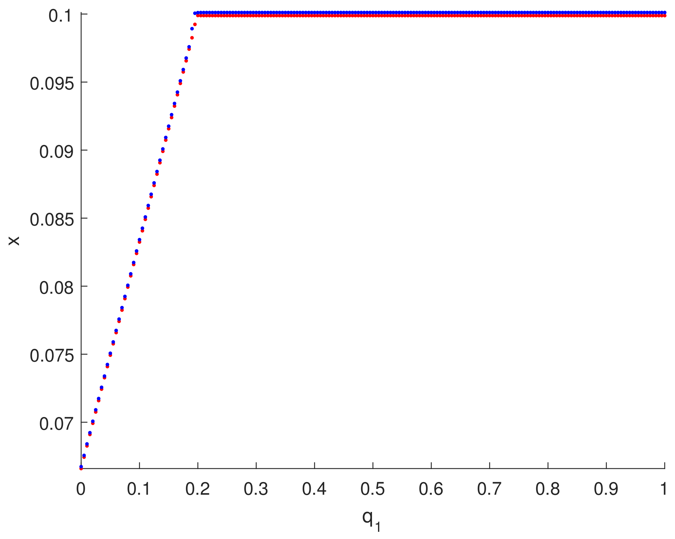
The effect of catchability constants can be shown by drawing the bifurcation diagram regarding $q_1$ as a bifurcation parameter. The transcritical bifurcation value is centered at $q_1^{*}=0.2$ as indicated in Figure 1. Note that the bifurcations that are presented in Theorem 5 are illustrated because $q_1^{*}=0.2$ is equivalent to $R_1=\frac{m_{1}k}{{\mu }_1+q_{1}E}=1$.

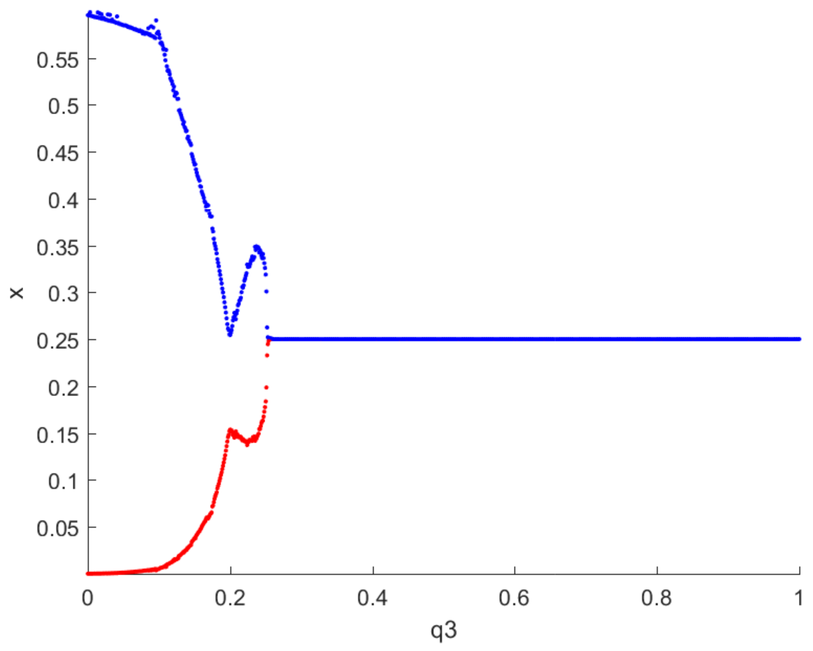
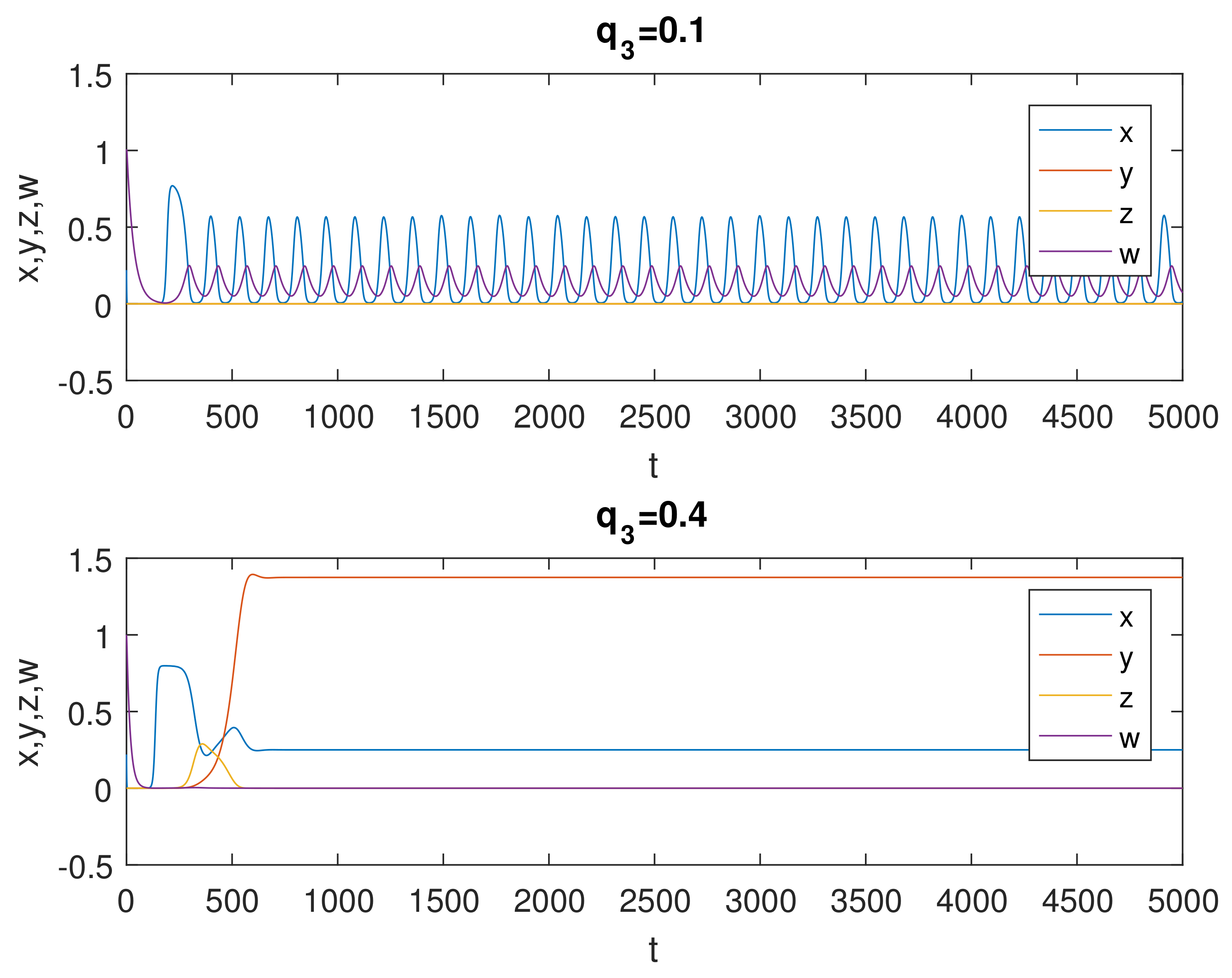
One can draw the bifurcation diagram regarding $q_3$ to indicate the effect of the harvesting. The supercritical Hopf bifurcation value is centered at $q_3^{*}=0.254669$ as indicated in Figure 2. It can also be noted that for $q_3>0.254669$, the prey–predator model (1) is locally stable as indicated in Figure 3, while for $q_3<0.254669$, the system goes through the limit cycle behavior. One can find that all the conditions of Theorem 14 hold as ${\Phi }_1\left(0.254669\right)=0,$${\Phi }_2\left(0.254669\right)\ne 0$ and $\frac{d{\Phi }_1\left(q_3\right)}{d{q}_3}{|}_{q_3=0.254669}\ne 0$. This confirms the existence of a Hopf bifurcation at $q_3^{*}=0.254669$. As a result, the harvesting parameter $q_3$ can break the oscillating behavior of the deterministic system (1) and drive it to the required state. In the same way, the bifurcation of the system can be studied using the parameter $q_2$, as shown in Figure 4.

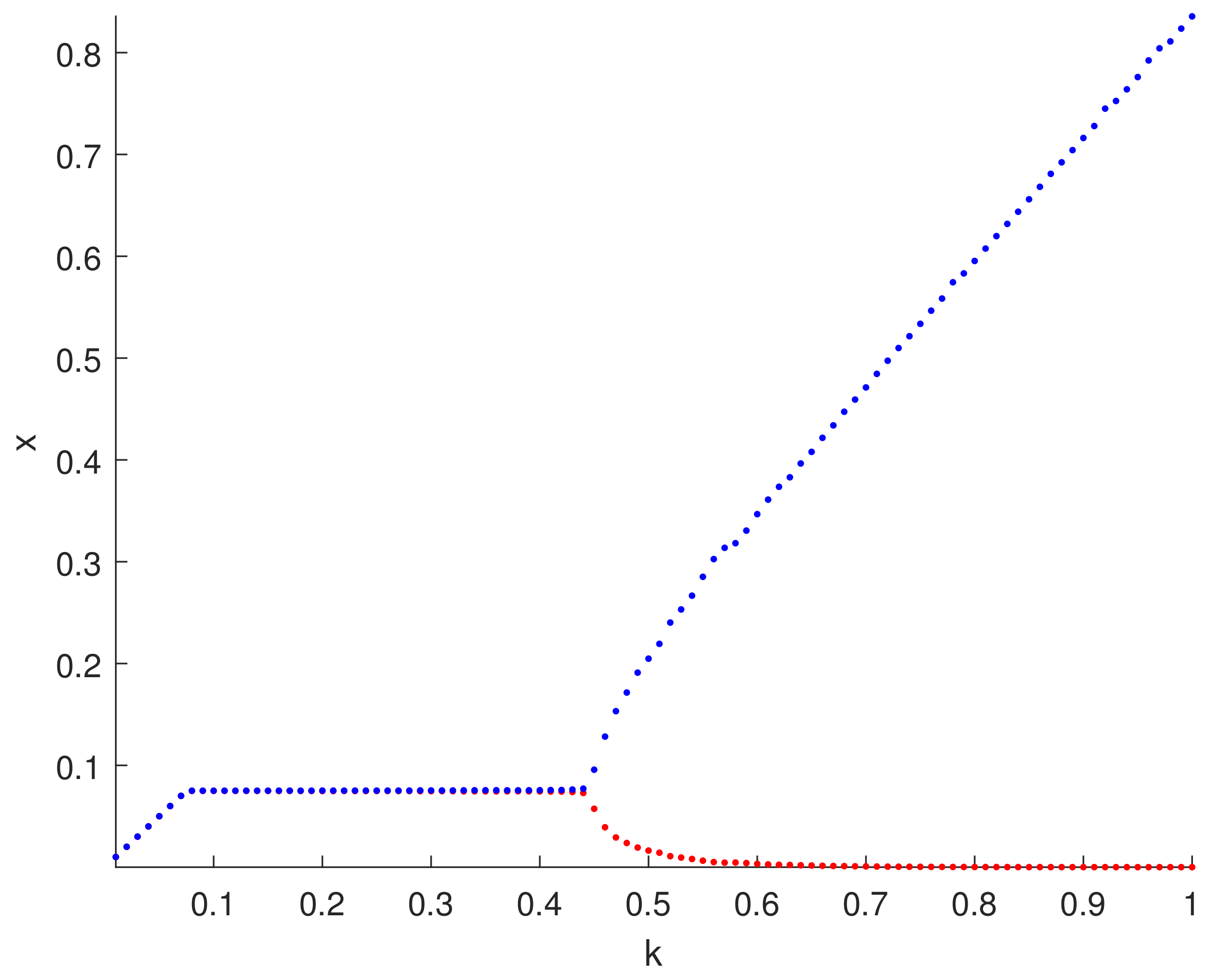
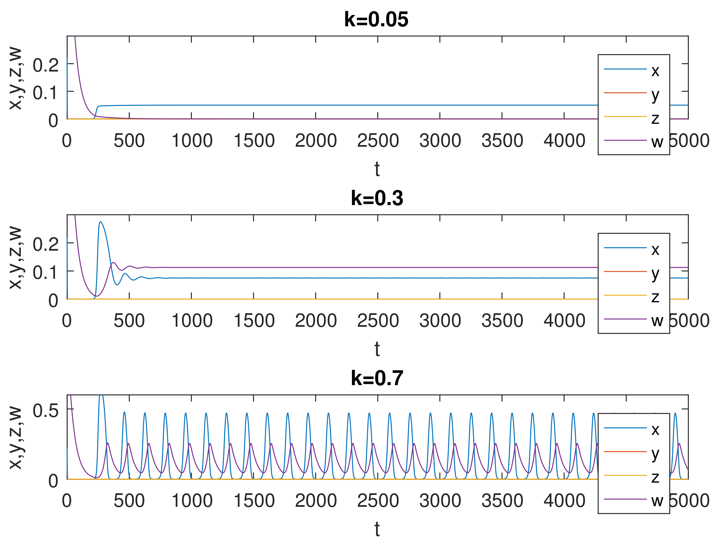
To better understand the effect of the caring capacity k, one can draw the bifurcation diagram with respect to k. It can be seen that the supercritical Hopf bifurcation value is localized at $k=0.45$ as shown in Figure 5. The supercritical Hopf bifurcation value is centered at $k=0.45$, as indicated in Figure 5. When $k>0.45$, the prey–predator model (1) goes through limit cycle oscillation, as indicated in Figure 5 and Figure 6. For $k<0.45$, $E_4=(0.075,0,0,0.15-0.01125/k)$ is locally stable, as indicated in Figure 6. It can also be noted that the conditions of local stability that were established in Theorem 10 were verified because when $k=0.4$, one has $R_3=2.8571<1+\frac{\left(a{m}_3\right)}{\left(({\mu }_3+q_{3}E)(a+k)\right)}=3.1429$.

To give some numerical findings for the prey predator system (8), one can use the Milstein method mentioned in [31,32]. The prey–predator system (8) reduces to the following discrete system.

$$\begin{array}{c}\hfill \begin{array}{cc}\hfill x_{j+1}& =x_j+h{x}_j\left(r(1-\frac{x_j}{k})-{\beta }_1{y}_j-{\beta }_2{z}_j-\frac{{\beta }_3{w}_j}{a+x_j}\right)+{\sigma }_1{x}_j\sqrt{h}{ϵ}_{1j}+\frac{{\sigma }_1^2}{2}{x}_j\left[{ϵ}_{1j}^2-1\right]h,\hfill \\ \hfill y_{j+1}& =y_j+h{y}_j\left(m_1{x}_j+\delta z_j-{\mu }_1-q_{1}E\right)+{\sigma }_2{y}_j\sqrt{h}{ϵ}_{2j}+\frac{{\sigma }_2^2}{2}{y}_j\left[{ϵ}_{2j}^2-1\right]h,\hfill \\ \hfill z_{j+1}& =z_j+h{z}_j\left(m_2{x}_j-\delta y_j-{\mu }_2-q_{2}E\right)+{\sigma }_3{z}_j\sqrt{h}{ϵ}_{3j}+\frac{{\sigma }_3^2}{2}{z}_j\left[{ϵ}_{zj}^2-1\right]h,\hfill \\ \hfill w_{j+1}& =w_j+h{w}_j\left(\frac{m_3{x}_j}{a+x_j}-{\mu }_3-q_{3}E\right)+{\sigma }_4{w}_j\sqrt{h}{ϵ}_{4j}+\frac{{\sigma }_4^2}{2}{w}_j\left[{ϵ}_{4j}^2-1\right]h,\hfill \end{array}\end{array}$$

(19)

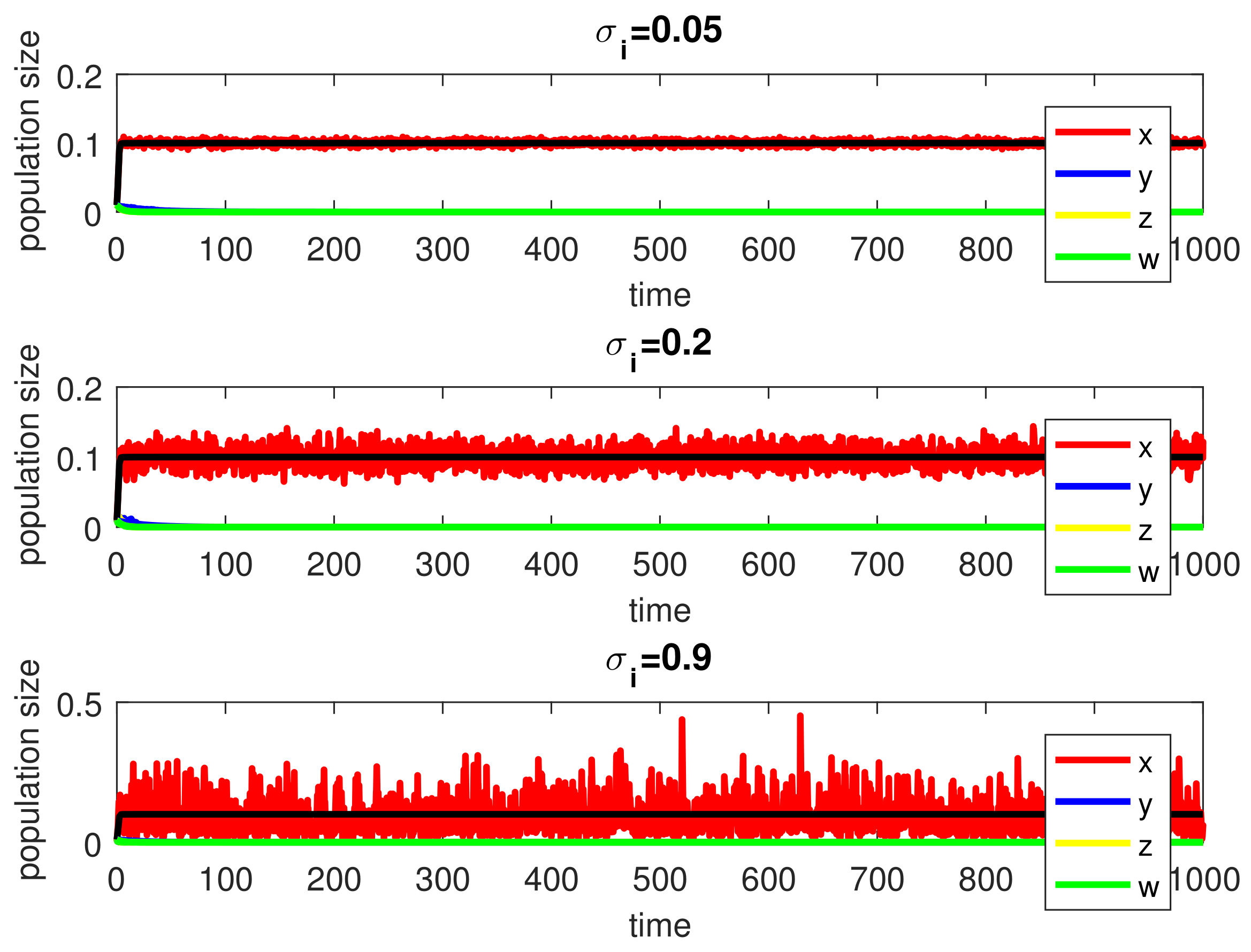
where h is a positive time increment and ${ϵ}_{ij},(i=1,2,3,4)$ are independent random Gaussian variables $N(0,1)$. Figure 7 represents the dynamical behavior of the model (8) when the noise strength is the law (${\sigma }_i=0.05$). One can note that for the given parameters, the strength of environmental noise is very close to zero, and the system behaves as a deterministic model. Following [33], one can note that in the deterministic case, if $R_0<1$, then the prey–predator system (1) has a predators’ free equilibrium point $E_1=(k,0,0,0)$. In the stochastic model (14), if one gradually increases the intensities of fluctuation and keeps the remaining parameters unchanged, the fluctuations around $E_1$ become larger, as seen for the values of ${\sigma }_i=0.2$ and $0.9$ shown in Figure 7. The black line in Figure 7 represents the prey when (${\sigma }_i=0$). From Figure 8, it is seen that increasing the catchability constants has a stabilizing effect on the stochastic model (14).

7. Conclusions

In this paper, a mathematical prey–predator model was proposed and analyzed. The interference of the predators in the system investigated in [12] was modified by adding an extra predator $y\left(t\right)$ where the first predator preys on the second predator in addition to the prey. The interaction between the three predators and single prey was studied. The impact of harvesting on the first and the second predator was investigated. Sufficient conditions were obtained to ensure local stability. It was concluded that the dynamics of the population can be controlled by harvesting. The harvesting rates of the three predator species played an important role in controlling the local and global dynamics of the prey–predator system. They can break the oscillating behavior of the deterministic system and drive it to the required state. To investigate the effect of environmental noise, we performed a stochastic extension of the deterministic model to study the fluctuation of the ecological factors. The existence of a unique global positive solution for the stochastic model was investigated. We used stochastic perturbation around the free predators’ equilibrium point. Constructing an appropriate Lyapunov function and applying Itô’s formula, we note that the deterministic model was robust with respect to stochastic perturbation. The criterion of stochastic stability depends on the intensities of noise ${\sigma }_i,i=1,2,3,4$. The exponential–mean–squared stability of the resulting stochastic differential equation model was examined, and it was found to be dependent on the harvesting effort.

References

1. Wikan, A.; Kristensen, Ø. Prey–predator interactions in two and three species population models. Discret. Dyn. Nat. Soc. 2019, 2019, 9543139. [Google Scholar] [CrossRef]
2. Sayekti, I.; Malik, M.; Aldila, D. One–prey two–predator model with prey harvesting in a food chain interaction. In Proceedings of the International Symposium on Current Progress in Mathematics and Sciences 2016 (ISCPMS 2016), AIP Conference Proceedings, Depok, Indonesia, 1–2 November 2016; AIP Publishing LLC: College Park, MD, USA, 2017; Volume 1862, p. 030124. [Google Scholar]
3. Ghosh, U.; Sarkar, S.; Mondal, B. Study of Stability and Bifurcation of Three Species Food Chain Model with Non–monotone Functional Response. Int. J. Appl. Comput. Math. 2021, 7, 63. [Google Scholar] [CrossRef]
4. Pal, D.; Kar, T.K.; Yamauchi, A.; Ghosh, B. Balancing maximum sustainable yield and ecological resilience in an exploited two–predator one–prey system. Biosystems 2020, 187, 104064. [Google Scholar] [CrossRef] [PubMed]
5. Kaviya, R.; Muthukumar, P. Dynamical analysis and optimal harvesting of conformable fractional prey–predator system with predator immigration. Eur. Phys. J. Plus 2021, 136, 136. [Google Scholar]
6. Fattahpour, H.; Zangeneh, H.R.; Nagata, W. Dynamics of Rodent Population With Two Predators. Bull. Iran. Math. Soc. 2019, 45, 965–996. [Google Scholar] [CrossRef]
7. Li, H.; Zhang, L.; Hu, C.; Jiang, Y.; Teng, Z. Dynamical analysis of a fractional-order predator-prey model incorporating a prey refuge. J. Appl. Math. Comput. 2016, 54, 435–449. [Google Scholar] [CrossRef]
8. Sambath, M.; Ramesh, P.; Balachandran, K. Asymptotic Behavior of the Fractional Order three Species Prey–Predator Model. Int. J. Nonlinear Sci. Numer. Simul. 2018, 19, 721–733. [Google Scholar] [CrossRef]
9. Das, D.K.; Das, K.; Kar, T. Dynamical Behaviour of Infected Predator–Prey Eco–epidemics with Harvesting Effort. Int. J. Appl. Comput. Math. 2021, 7, 66. [Google Scholar] [CrossRef]
10. Mondal, S.; Samanta, G. Impact of fear on a predator–prey system with prey-dependent search rate in deterministic and stochastic environment. Nonlinear Dyn. 2021, 104, 2931–2959. [Google Scholar] [CrossRef]
11. Zhang, Y.; Tian, B.; Chen, X.; Li, J. A stochastic diseased predator system with modified LG–Holling type II functional response. Ecol. Complex. 2021, 45, 100881. [Google Scholar] [CrossRef]
12. Mukhopadhyay, B.; Bhattacharyya, R. Effects of harvesting and predator interference in a model of two–predators competing for a single prey. Appl. Math. Model. 2016, 40, 3264–3274. [Google Scholar] [CrossRef]
13. Garneau, D.E.; Post, E.; Boudreau, T.; Keech, M.; Valkenburg, P. Spatio–temporal patterns of predation among three sympatric predators in a single–prey system. Wildl. Biol. 2007, 13, 186–194. [Google Scholar] [CrossRef] [Green Version]
14. Cresson, J.; Szafrańska, A. Discrete and continuous fractional persistence problems—The positivity property and applications. Commun. Nonlinear Sci. Numer. Simul. 2017, 44, 424–448. [Google Scholar] [CrossRef] [Green Version]
15. Perko, L. Differential Equations and Dynamical Systems; Springer Science & Business Media: New York, NY, USA, 2013; Volume 7. [Google Scholar]
16. Wiggins, S.; Golubitsky, M. Introduction to Applied Nonlinear Dynamical Systems and Chaos; Springer: New York, NY, USA, 2003; Volume 2. [Google Scholar]
17. Maji, C.; Mukherjee, D.; Kesh, D. Deterministic and stochastic analysis of an eco–epidemiological model. J. Biol. Phys. 2018, 44, 17–36. [Google Scholar] [CrossRef]
18. Cresson, J.; Puig, B.; Sonner, S. Stochastic models in biology and the invariance problem. Discret. Contin. Dyn. Syst. B 2016, 21, 2145. [Google Scholar] [CrossRef] [Green Version]
19. Cresson, J.; Sonner, S. A note on a derivation method for SDE models: Applications in biology and viability criteria. Stoch. Anal. Appl. 2018, 36, 224–239. [Google Scholar] [CrossRef]
20. Phan, T.A.; Tian, J.P.; Wang, B. Dynamics of cholera epidemic models in fluctuating environments. Stoch. Dyn. 2021, 21, 2150011. [Google Scholar] [CrossRef]
21. Mao, X. Stochastic Differential Equations and Applications; Woodhead Publishing: Cambridge, UK, 2007. [Google Scholar]
22. Cai, Y.; Mao, X. Stochastic prey–predator system with foraging arena scheme. Appl. Math. Model. 2018, 64, 357–371. [Google Scholar] [CrossRef] [Green Version]
23. Wei, C.; Liu, J.; Zhang, S. Analysis of a stochastic eco–epidemiological model with modified Leslie–Gower functional response. Adv. Differ. Equ. 2018, 2018, 119. [Google Scholar] [CrossRef] [Green Version]
24. Liu, Q.; Jiang, D.; Hayat, T.; Alsaedi, A.; Ahmad, B. A stochastic SIRS epidemic model with logistic growth and general nonlinear incidence rate. Phys. A Stat. Mech. Appl. 2020, 551, 124152. [Google Scholar] [CrossRef]
25. Li, Q.; Cong, F.; Liu, T.; Zhou, Y. Stationary distribution of a stochastic HIV model with two infective stages. Phys. A Stat. Mech. Appl. 2020, 554, 124686. [Google Scholar] [CrossRef]
26. Afanasiev, V.N.; Kolmanovskii, V.; Nosov, V. Mathematical Theory of Control Systems Design; Springer Science & Business Media: Dordrecht, The Netherlands, 2013; Volume 341. [Google Scholar]
27. Mukhopadhyay, B.; Bhattacharyya, R. A nonlinear mathematical model of virus–tumor–immune system interaction: Deterministic and stochastic analysis. Stoch. Anal. Appl. 2009, 27, 409–429. [Google Scholar] [CrossRef]
28. Mukhopadhyay, B.; Bhattacharyya, R. On a three–tier ecological food chain model with deterministic and random harvesting: A mathematical study. Nonlinear Anal. Model. Control. 2011, 16, 77–88. [Google Scholar] [CrossRef] [Green Version]
29. Mukhopadhyay, B.; Bhattacharyya, R. Effects of deterministic and random refuge in a prey–predator model with parasite infection. Math. Biosci. 2012, 239, 124–130. [Google Scholar] [CrossRef]
30. Ghosh, P.; Das, P.; Mukherjee, D. Persistence and stability of a seasonally perturbed three species stochastic model of salmonoid aquaculture. Differ. Equ. Dyn. Syst. 2019, 27, 449–465. [Google Scholar] [CrossRef]
31. Higham, D.J. An algorithmic introduction to numerical simulation of stochastic differential equations. SIAM Rev. 2001, 43, 525–546. [Google Scholar] [CrossRef]
32. Alnafisah, Y. The implementation of Milstein scheme in two–dimensional SDEs using the Fourier method. Abstr. Appl. Anal. 2018, 2018, 3805042. [Google Scholar] [CrossRef] [Green Version]
33. Cao, Y.; Denu, D. Analysis of stochastic vector–host epidemic model with direct transmission. Discret. Contin. Dyn. Syst. B 2016, 21, 2109–2127. [Google Scholar] [CrossRef] [Green Version]
Figure 1. Bifurcation diagram of the model (1) with respect to q 1 .
Axioms 11 00156 g001
Figure 2. Bifurcation diagram of the model (1) with respect to q 3 .
Axioms 11 00156 g002
Figure 3. Time series of the model (1) with q 3 = 0.1 and q 3 = 0.4 .
Axioms 11 00156 g003
Figure 4. Bifurcation diagram of the model (1) with respect to q 2 .
Axioms 11 00156 g004
Figure 5. Bifurcation diagram of the model (1) with respect to k.
Axioms 11 00156 g005
Figure 6. Time series of the model (1) with k = 0.05 , k = 0.3 , and k = 0.7 .
Axioms 11 00156 g006
Figure 7. Fluctuation in the prey population with σ i = 0.05 , σ i = 0.2 , and σ i = 0.9 . The black line represents the prey when ( σ i = 0 ).
Axioms 11 00156 g007
Figure 8. Numerical simulation of the system (14) with ( q 1 = q 2 = q 3 = 0.1 ) and ( q 1 = q 2 = q 3 = 0.5) .
Axioms 11 00156 g008
Publisher’s Note: MDPI stays neutral with regard to jurisdictional claims in published maps and institutional affiliations.