A Modified Ant Lion Optimization Method and Its Application for Instance Reduction Problem in Balanced and Imbalanced Data

Abstract

Instance reduction is a pre-processing step devised to improve the task of classification. Instance reduction algorithms search for a reduced set of instances to mitigate the low computational efficiency and high storage requirements. Hence, finding the optimal subset of instances is of utmost importance. Metaheuristic techniques are used to search for the optimal subset of instances as a potential application. Antlion optimization (ALO) is a recent metaheuristic algorithm that simulates antlion’s foraging performance in finding and attacking ants. However, the ALO algorithm suffers from local optima stagnation and slow convergence speed for some optimization problems. In this study, a new modified antlion optimization (MALO) algorithm is recommended to improve the primary ALO performance by adding a new parameter that depends on the step length of each ant while revising the antlion position. Furthermore, the suggested MALO algorithm is adapted to the challenge of instance reduction to obtain better results in terms of many metrics. The results based on twenty-three benchmark functions at 500 iterations and thirteen benchmark functions at 1000 iterations demonstrate that the proposed MALO algorithm escapes the local optima and provides a better convergence rate as compared to the basic ALO algorithm and some well-known and recent optimization algorithms. In addition, the results based on 15 balanced and imbalanced datasets and 18 oversampled imbalanced datasets show that the instance reduction proposed method can statistically outperform the basic ALO algorithm and has strong competitiveness against other comparative algorithms in terms of four performance measures: Accuracy, Balanced Accuracy (BACC), Geometric mean (G-mean), and Area Under the Curve (AUC) in addition to the run time. MALO algorithm results show increment in Accuracy, BACC, G-mean, and AUC rates up to 7%, 3%, 15%, and 9%, respectively, for some datasets over the basic ALO algorithm while keeping less computational time.

1. Introduction

Machine Learning plays a crucial role in extracting useful information in different research domains, for instance, medical data analysis [1,2,3,4], computer vision [5], road accident analysis [6], educational data mining [7], sentiment analysis [8] and many more. Instance reduction is one of the prime pre-processing tasks in machine learning applications. Before employing instance-based learning methods, alleviating the noisy, erroneous, and redundant data are highly desirable. Instance reduction mitigates sensitivity to noise and high storage requirements. Eventually, the complication of calculation to understand a superior classification technique decline. There should not be a noteworthy change in between-class distribution after and before data decline. A flawed data reduction technique may eradicate additional instances of one class, resulting in unfair datasets.

Instance reduction can be applied for both balanced and imbalanced data to improve classification performance. Researchers studied the instance decline from class-balanced data. However, there are not many studies on class-imbalanced data. Researchers attract to this issue in recent times because of practical applications in this domain [9]. The imbalanced dataset poses difficulties in learning tasks. Traditional methods are exploited to learn from imbalanced data. Satisfactory outcomes are not yielded as these traditional methods execute excellent coverage for the mainstream class while marginal classes are disregarded. In some cases, high accuracies are demonstrated, but the outcome is not as trustworthy as the cardinality of the majority class is high contrasted to the minority class. For instance, the reduction to keep intact between-class distribution is vital. In imbalanced datasets, the minority class instances are also essential. Such instances may be treated as noise or outliers. However, these minority class instances must not be lessened while applying an instance reduction method. Hence, to take care of that, special techniques are needed.

Among different instance reduction methods for imbalanced data, data-level methods are of utmost importance. These data-level techniques can be classified into two types: oversampling, the size of the marginal class is enhanced and under-sampling, the size of the mainstream class is lessened, ensemble-based methods, and cost-sensitive methods. Various research papers suggested that evolutionary-based techniques performed better than the non-evolutionary ones in imbalanced dataset analysis and instance reduction.

Researchers have gained interest over the years to locate optimal values of the solution variables to meet definite conditions in case of global optimization concerns. Gigantic computational efforts are required for classical optimization methods that are inclined to be unsuccessful as the problem search space escalates. Meta-heuristic algorithms have come into the picture that exhibits better computational efficacy in evading local minima [10]. These meta-heuristic algorithms showcased their superiority for tackling complex issues in different domains for the subsequent causes. (i) They can circumvent local minima; (ii) the gradient of the objective function is not needed; (iii) they are easy to implement and simple; (iv) different problems of various fields can be solved by utilizing it. The increasing processing power of computers has a positive impact on the development of such algorithms.

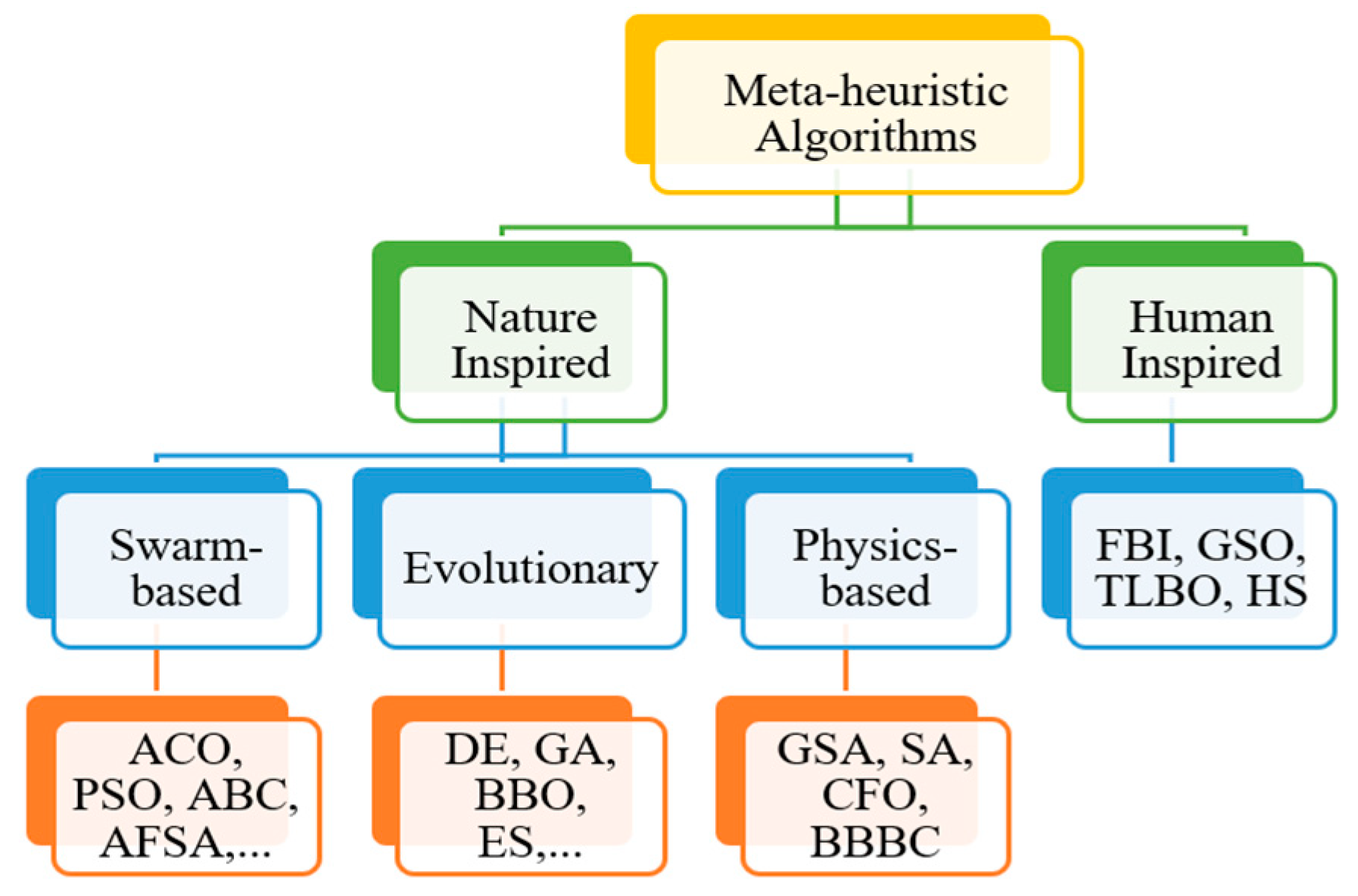
The metaphors applied in metaheuristic techniques are plants, humans, birds, the ecosystem, water, gravitational forces, and electromagnetic forces. As described in Figure 1, it can be divided into two categories. The first category mimics physical or biological phenomena and three sub-categories come into existence from it. They are swarm-based, physics-based, and evolution-based techniques. Human phenomena are the main inspiration behind the second category.

Abbreviations: ACO: Ant Colony Optimization, PSO: Particle Swarm Optimization, ABC: Artificial Bee Colony, AFSA: Artificial Fish Swarm Algorithm, DE: Differential Evolution, GA: Genetic Algorithm, BBO: Biogeography-Based Optimizer, ES: Evolution Strategy, GSA: Gravitational Search Algorithm, SA: Simulated Annealing, CFO: Central Force Optimization, BBBC: Big-Bang Big-Crunch, FBI: Forensic-Based Investigation, GSO: Group Search Optimizer, TLBO: Teaching-Learning-Based Optimization, HS: Harmony Search.

Metaheuristic techniques were utilized for different real-world applications, Negi et al. [11] proposed a hybrid approach with PSO and GWO methods and dubbed it HPSOGWO to tackle optimization problems and reliability allocation of life support systems and Complex bridge systems. In [12], the authors devised a modified genetic algorithm (MGA) with a novel selection method, namely a generation-dependent mutation and an in-vitro-fertilization-based crossover. They applied their technique in commercial ship scheduling and routing with dynamic demand and supply environments. Their model could lessen risks and abate port time with a static load factor. Ganguly in [13] proposed a framework for simultaneous optimization of Distributed Generation (DG) network performance index and penetration level to acquire the optimal sizes, numbers, and sites of DG units. He formulated two objective functions. Network performance index and DG penetration level were the two. Multi-objective particle swarm optimization was utilized by his solution framework and was validated on a distribution system comprising 38 nodes.

In [14], the authors implemented a general type-2 fuzzy classification method for the medical assistance and the optimization of the general type-2 membership functions parameters using ALO for comparison these two type classifiers with the Framingham dataset. A general type-2 fuzzy classifier had been applied on the Jetson Nano hardware Development Board and execution time of the type-1 and type-2 fuzzy classification techniques were compared. A novel metaheuristic method called the Slime Mold Algorithm (SMA) was proposed in [15]. A fuzzy controller tuning technique is also offered and the concept of enhancing the performance of metaheuristics with information feedback approaches has been applied. The fuzzy controllers and their tuning methods were validated in real-time with angular position control of the laboratory servo framework. In [16], a survey was presented on scientific literature works that dealt with Type-2 fuzzy logic controllers devised utilizing nature-inspired optimization techniques. Their review exploited the most widespread optimizers to attain the key parameters on Type-2 and Type-1 fuzzy controllers to enhance the gained outcome. The PSO method was integrated in [17], with the Multi-Verse Optimizer (MVO) to classify endometrial carcinoma with gene expression by optimizing the parameters of the Elman neural network.

Swarm intelligence methods were also utilized for feature reduction. Gupta et al. [18] presented a revised antlion optimization procedure to better identify thyroid infection. To mitigate the computational time and enhance the classification accuracy, the proposed method was exploited as a feature reduction technique to detect the vital attributes from a large set of attributes. Their method had successfully eradicated 71.5% of irrelevant features. Based on Stochastic Fractal Search (SFS), El-Kenawy et al. [19] introduced a Modified Binary GWO (MbGWO) to determine key characteristics by attaining the exploitation and exploration balance. They tested their MbGWO-SFS method with 19 machine learning datasets from the University of California, Irvine (UCI). Comparison with the state-of-the-art optimization methods demonstrated the superiority of the method. Lin et al. [20] applied modified cat swarm optimization (CSO) that outperformed PSO. The limitation of CSO is that its computation time is long. Hence, their modified version was called ICSO. Their method selected features in big data-related text classification. To propose a feature selection method, Wan et al. [21] utilized a customized binary-coded ant colony optimization (MBACO) method in combination together with a genetic algorithm. Their technique comprised of two models, the pheromone density model (PMBACO) and the visibility density model (VMBACO). The results acquired by GA were applied as early pheromone evidence in the PMBACO model, whereas the solution attained by GA was employed as visibility information in the VMBACO model. Based on the modified grasshopper optimization method, Zakeri et al. [22] devised a new feature selection technique. The novel method dubbed Grasshopper Optimization Algorithm for Feature Selection (GOFS) replicated the duplicate features with promising features by applying statistical techniques while performing iterations.

Instance reduction is a pre-processing task devised to improve learning jobs. Nanni et al. [23] developed an effective technique based on particle swarm optimization for prototype reduction. Their technique minimized the error rate on the training set. Zhai et al. [24] introduced a novel immune binary particle swarm optimization technique for time series classification, which searched for the smallest instance combination with the highest classification accuracy. Hamidzadeh et al. [25] presented a Large Margin Instance Reduction Algorithm (LMIRA) that kept border instances and removed the non-border ones. The algorithm considered the instance reduction issue as a constrained binary optimization problem, and a filled function algorithm was exploited to tackle the issue. The reduction process’s basic was relied on the hyperplane that separated the two-class data and demonstrated large margin separation. Saidi et al. [26] proposed a novel instance selection method dubbed Ensemble Margin Instance Selection (EMIS). The ensemble margin was employed in their method. They applied their method for automatic recognition and selection of white blood cells WBC in cytological images.

Carbonera and Abel [27] devised an effective and simple density-based framework for instance collection termed local density-based instance selection (LDIS). Their technique kept the densest instances in an arbitrary neighborhood by examining the instances of each class. For evaluating the accuracy, they applied the K-Nearest Neighbor (KNN) algorithm. de Haro-García et al. [28] utilized boosting method to obtain reduced instances to achieve better accuracy. The stepwise addition of instances was performed by applying the weighting of instances from the building of ensembles of classifiers.

Numerous modified versions of Antlion optimizers have been proposed for solving different research problems. In [29], Wang et al. proposed an enhanced alternate method for Antlion Optimizer (ALO), incorporating opposition-based training with two functional operators centered on differential evolution, named MALO, which is suggested to deal with the implicit vulnerabilities of conventional ALO. Pierezan et al. [30] suggested four multi-objective ALO (MOALO) methods utilizing swarming distance, supremacy idea for choosing the elite, and tournament collection techniques with various programs to pick the chief. Assiri et al. [31] showed the benefits and different categories like Modified, Hybrid, and Multi-Objective of ALO algorithms after giving a detailed introduction of this procedure. This paper also discussed the applications and foundations of this method and finished with some suggestions and possible directions in the future.

In the literature, different metaheuristic and optimization algorithms were proposed to enhance the performance of classification using the instance reduction issue. However, as far as the authors are aware, this is the first time ALO algorithm or a modified version of it is proposed to solve the instance reduction issue in balanced and imbalanced data. In this paper, MALO will be utilized to enhance the ALO’s ability to escape the local optima while providing a better convergence rate and enhancing the classification performance in real-world datasets by optimized instance reduction.

The main contributions of this work are summarized as follows:

(1) Since the ALO algorithm suffers from local optima stagnation and slow convergence speed for some optimization problems [32], this study’s intention is to propose a new modified antlion optimization (MALO) algorithm to enhance the optimization efficiency and accuracy of ALO by adding a new parameter depends on the step length of each ant while updating the antlion position based on the parameter, upper and lower bounds of search space.

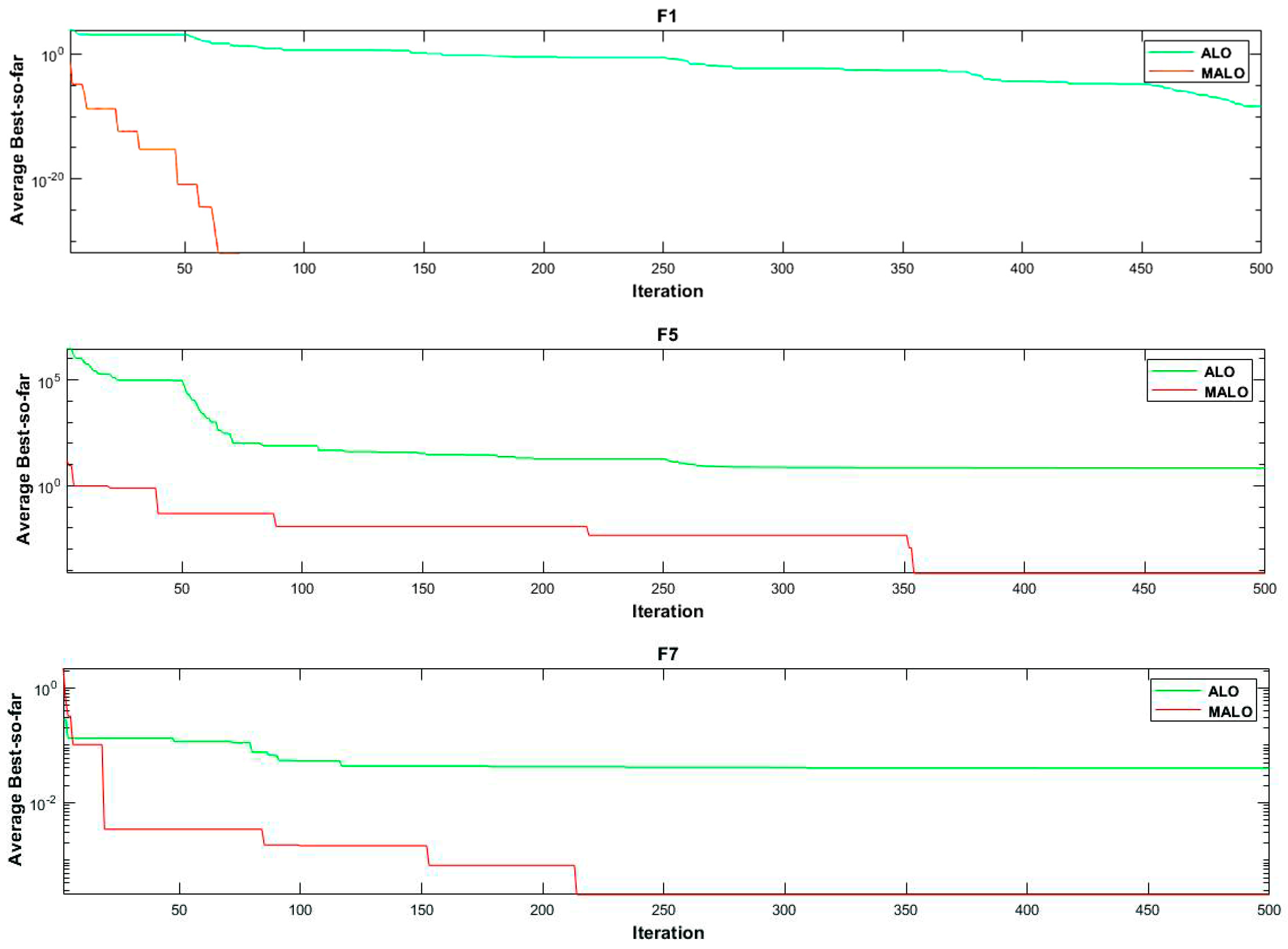
(2) The proposed MALO algorithm is tested on twenty-three benchmark functions at 500 iterations and thirteen benchmark functions at 1000 iterations. The results provide evidence that the suggested MALO escapes the local optima and provides a better convergence rate as compared to the basic ALO algorithm, some well-known and recent optimization algorithms.

(3) Furthermore, 15 balanced and imbalanced datasets were employed to test the performance of the proposed MALO algorithm on reducing instances of the training data and the results are compared with some well-known optimization algorithms.

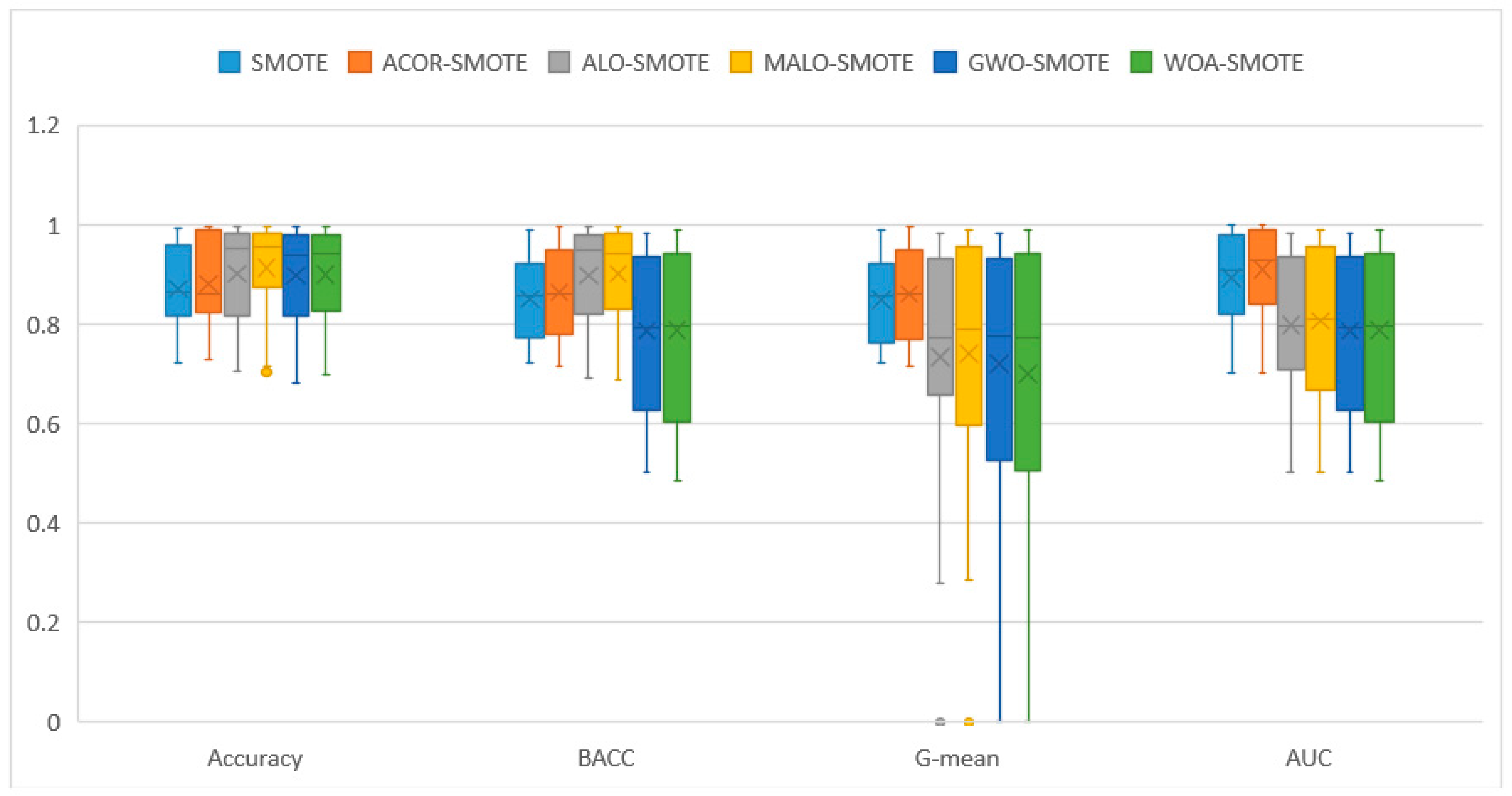
(4) The Wilcoxon signed-rank test is also applied. The results showcase that the proposed instance reduction method statistically outperforms the MALO algorithm and other comparable optimization techniques based on the recorded Accuracy, BACC, G-Mean, and AUC metrics while keeping less computational time.

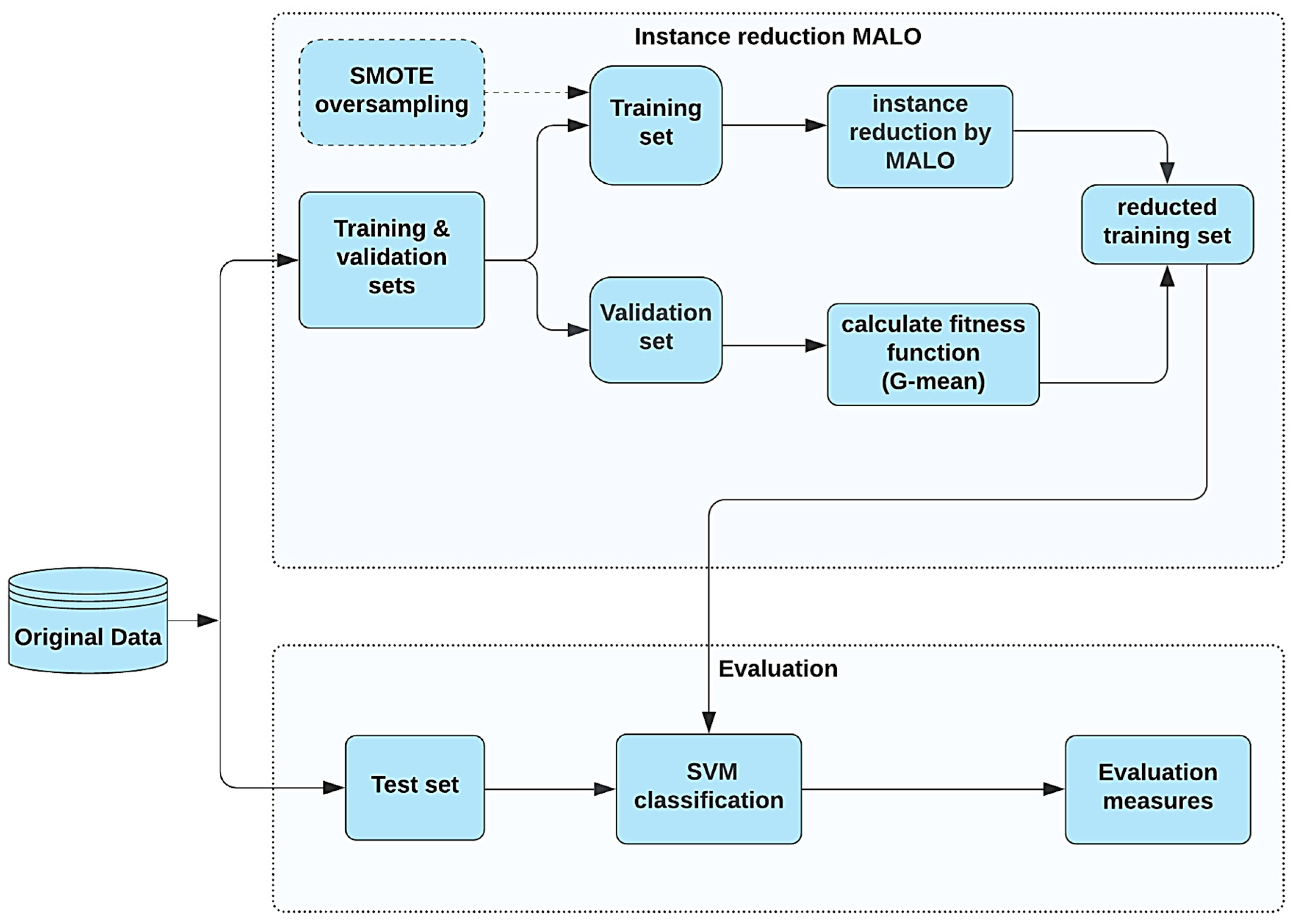
(5) Moreover, antlion optimization and MALO were used to perform training data reduction for 18 oversampled imbalanced datasets, and learning is performed using Support Vector Machines (SVM) classifier in all performed experiments. The results are compared with one novel resampling method and two recent algorithms.

2. Methodology

2.1. Antlion Optimizer

Seyedali Mirjalili proposed an Antlion Optimizer (ALO) in 2015 utilizing the ant and lions hunting process [33]. This method consists of five major steps of hunting, specifically random walk of agents, entrapment of ants in the trap, constructing traps, reconstructing traps, and capturing prey. Ant and antlion interactions are followed in the ALO algorithm where the ants are chased by antlions utilizing the traps, and ants are authorized to drift into the search area stochastically for food.

The following matrices represent the matrices for representing the place of p ants and p antlions, where q is the number of variables (dimension).

$$S_{Ant}=\left[\begin{array}{cccc}An{t}_{1,1}& An{t}_{1,2}& \dots & An{t}_{1,q}\\ An{t}_{2,1}& An{t}_{2,2}& \dots & An{t}_{2, q}\\ \dots & \dots & \dots & \dots \\ An{t}_{p, 1}& An{t}_{p,2}& \dots & An{t}_{p,q}\end{array}\right]$$

(1)

and

$$S_{Antlion}=\left[\begin{array}{cccc}Antlio{n}_{1,1}& Antlio{n}_{1,2}& \dots & Antlio{n}_{1,q}\\ Antlio{n}_{2,1}& Antlio{n}_{2,2}& \dots & Antlio{n}_{2, q}\\ \dots & \dots & \dots & \dots \\ Antlio{n}_{p, 1}& Antlio{n}_{p,2}& \dots & Antlio{n}_{p,q}\end{array}\right]$$

(2)

If f indicated the fitness function for the duration of optimization, then the matrices developed the matrices for savings the fitness value (objective) of p ants (S_OAnt) and p antlions (S_OAntlion).

$$S_{OAnt}=\left[\begin{array}{c}\begin{array}{c}f\left(\left[An{t}_{11},An{t}_{12},\dots , An{t}_{1q}\right]\right)\\ f\left(\left[An{t}_{21},An{t}_{22},\dots , An{t}_{2q}\right]\right)\\ \dots \end{array}\\ f\left(\left[An{t}_{p1},An{t}_{p2},\dots ,An{t}_{pq}\right]\right)\end{array}\right]$$

(3)

and

$$S_{OAntlion}=\left[\begin{array}{c}\begin{array}{c}f\left(\left[Antlio{n}_{11},Antlio{n}_{L12},\dots , Antlio{n}_{1q}\right]\right)\\ f\left(\left[Antlio{n}_{21},Antlio{n}_{22},\dots , Antlio{n}_{2q}\right]\right)\\ \dots \end{array}\\ f\left(\left[Antlio{n}_{p1},Antlio{n}_{p2},\dots , Antlio{n}_{pq}\right]\right)\end{array}\right]$$

(4)

ALO algorithm contains six operators.

(i) Random Walks of Ants. At every single stage of optimization, ants revise their places with a random walk X(t). A random walk is calculated according to Equation (5). Where the cumulative sum is computed by cumsum, the maximum number of iterations is T, the present repetition (iteration) is indicated by t and rand implies a random number using the uniform probability distribution with the range [0, 1].

$$X\left(t\right)=[0,\mathit{cumsum}(2r(t_1)-1),\mathit{cumsum}\left(2r\right(t_2)-1),\dots ,\mathit{cumsum}\left(2r\right(t_T)-1)]$$

(5)

where the statistic function r(t) is illustrated as in Equation (6).

$$r(t)=\left\{\begin{array}{c}1\hspace{1em}if\hspace{1em}rand>0.5\\ \\ 0\hspace{1em}if\hspace{1em}rand\le 0.5\end{array}\right.$$

(6)

The ants are normalized as each search area has a province to maintain the random walks within the search area. To normalize the process the subsequent equation (min-max normalization), Equation (7) is used before updating the position of ants. Where the lowest of random walk of the ith variable is $a_i$, $q_i$ is the highest of random walk in the ith variable, $c_i^t$ implies the smallest of the ith variable at the tth repetition, $q_i^t$ implies the highest of the ith variable at the tth repetition.

$$X_i^t=\frac{\left(X_i^t-a_i\right)\times \left(q_i-c_i^t\right)}{\left(q_i^t-a_i\right)}+c_i^t$$

(7)

(ii) Trapping in Antlion’s Pits. The traps of Antlions affect the random walks of ants. Equations (8) and (9) illustrate that ant’s random walk in a hypersphere is indicated by the c and q vectors across a chosen antlion.

In these equations, $l{c}^t$ implies the lowest among total variables at the tth repetition, the vector ${hq}^t$ suggests involving the vector of the highest of total variables at the tth repetition, $c_i^t$ implies the lowest of total variables for the ith ant, $q_i^t$ indicates the highest of total variables for the ith ant, and $Antlio{n}_j^t$ indicates a place of chosen jth antlion of tth repetition. Where i is the index of the current ant and j is the index of the current antlion.

$$c_i^t=Antlio{n}_j^t+l{c}^t$$

(8)

and

$$q_i^t=Antlio{n}_j^t+h{q}^t$$

(9)

(iii) Building Trap. To choose the fitter antlions intended for capturing ants founded on the fitness value for the period of optimization, a roulette wheel in the ALO procedure is utilized.

(iv) Sliding Ants towards Antlion. Antlions can develop traps proportionately and ants change arbitrarily corresponding to the fitness values. Antlions shoot sands outwards when the ants are in the trap in the middle of the pit. This performance slides down the stuck ant, which is attempting to avoid the trap; in this circumstance, the range of the ants’ random walks hypersphere is reduced adjustably. Considering $r{c}^t$ and $r{q}^t$ as the reduced vectors of the lowest and highest random walks among total variables at the tth repetition, respectively:

$$r{c}^t=\frac{l{c}^t}{I}$$

(10)

and

$$r{q}^t=\frac{h{q}^t}{I}$$

(11)

where $l{c}^t$ implies the lowest among total variables at the tth repetition, the vector ${hq}^t$ suggests involving the vector of the highest of total variables at the tth repetition, and I indicate a ratio that calculated as:

$$I={10}^w(t/T)$$

where, w implies a fixed value indicated centered on the present reptation t [((w = 2, if t > 0.1 T), (w = 3 if t > 0.5 T), (w = 4 if t > 0.75 T), (w = 5 if t > 0.9 T) and (w = 6 if t > 0.95 T)]. Mostly, the fixed value w is able to accommodate the intensity of manipulation and precision.

Equations (10) and (11) decrease the range of the revising ants’ places and simulate the sliding method of an ant inside the pits.

(v) Catching Prey and Rebuilding the Pit. The ant gets caught by the antlion as soon as it goes to the underside of the pit. The antlion revises the place to the most recent situation of the tracked ant to enhance its probability of capturing new-found prey as in Equation (12):

$$Antlio{n}_j^t=An{t}_i^t iff\left(Antlio{n}_j^t\right)<f\left(An{t}_i^t\right)$$

(12)

where $Antlio{n}_j^t$ indicated the place of the chosen jth antlion at the tth repetition and $An{t}_i^t$ implies a place of the ith ant at the tth repetition.

(vi) Elitism. The essential feature of the evolutionary processes to preserve the finest explanation(s) achieved at every phase of the optimization procedure is elitism. The greatest antlion is an elite in the ALO procedure. Every single ant arbitrarily walks all over a carefully chosen antlion via the roulette wheel and the elite instantaneously as defined in Equation (13).

$$An{t}_i^t=\frac{R_A^t+R_E^t}{2}$$

(13)

In this equation, the random walk indicated by $R_A^t$ all over the antlion is chosen by the roulette wheel at the tth repetition, the random walk all over the elite is implied by $R_E^t$ at the tth repetition.

Let a function that produces the arbitrary primary results be X, Y directs the preliminary population presented by the function X, and Z comes back true when the ending principle is assured. Utilizing the above-recommended operations, the ALO procedure is identified as a three-tuple which can be shown as follows:

ALO (X, Y, Z)

(14)

where the functions X, Y, and Z are defined as follows

$$\varnothing \stackrel{X}{\to }\left\{S_{Ant}, S_{OAnt},S_{Antlion},S_{OAntlion}\right\}$$

(15)

$$\left\{S_{Ant}, S_{Antlion}\right\}\stackrel{Y}{\to }\left\{S_{Ant}, S_{Antlion}\right\}$$

(16)

$$\left\{S_{Ant}, S_{Antlion}\right\} \stackrel{Z}{\to }\left\{true, false\right\}$$

(17)

Here, $S_{Ant}$ implies the matrix of the place of the ants, $S_{Antlion}$ incorporates antlions’ place, $S_{O\mathit{Ant}}$ includes the ants’ consequent fitness, and $S_{O\mathit{Antlion}}$ has antlions’ fitness.

2.2. Modified Antlion Optimization (Malo) Method and Its Adaption for Instance Reduction

The ALO algorithm updates the ants’ positions based on random walks across the antlion which is elected by the roulette wheel and the elite. Then, by updating the elite during the method of searching, the fittest one is chosen. However, it suffers from local optima stagnation and slow convergence speed for some optimization problems [32]. MALO is proposed to enhance the optimization precision and effectiveness of ALO by adding a new parameter $Tu$ which depends on the step length of each ant while updating the antlion position based on the parameter $Tu$, upper and lower bounds of search space. The pseudocode of the MALO optimization method is presented in Algorithm 1.

Algorithm 1: Pseudocode of MALO.

Set number of antlions = number of ants = p, upper bounds of variables =$ub$, lower bounds of variables = $lb$, the maximum number of iterations = T, the present repetition (iteration) = t, rand implies a random number, $lc$ and $hq$ are vectors that represent the lowest and highest ant’s random walks, $R_A^t$ is a random walk all over the antlion chosen by the roulette wheel at the tth repetition and the random walk all over the elite is implied by $R_E^t$ at the tth repetition.

Randomly start the first population of the ants and the antlions

Compute the fitness of the ants and the antlions

Pinpoint the best antlions and presume it as determining optimum or the elite

While $(t<T)$

For $i=1 to p$ (number of ants or antlions)

$Tu=i/p$

$mu=10^\left(Tu\ast 100\right)$

Choose an antlion utilizing Roulette wheel

revise c and q applying Equations (10) and (11)

Construct a random walk and normalize it applying Equations (5) and (7)

%Generate a new position based on lower, upper bounds and a random proportional to the current position.

$yt=2\ast rand\ast \left(size\left(R_A^t\right)\right)-1$

$dx=(\left(\left(1+mu\right).^abs\left(yt\right)-1\right)/mu.\ast sign\left(yt\right).\ast \left(ub-lb\right)$

The position of the ant is updated using equation

$An{t}_i^t=(\frac{R_A^t+R_E^t}{2})/dx$

End For

Compute the fitness of all ants

An antlion is substituted by its subsequent ant if it becomes fitter (Equation (12))

If an antlion becomes fitter than the elite, then the elite is updated

End While

Return elite

For validating the MALO performance, it is tested using benchmark functions and applied for instance reduction on many real-world datasets.

The test is performed on benchmark functions to prove that the proposed MALO algorithm has the ability to escape the local optima and provides a better convergence rate compared to the basic ALO algorithm and some other well-known optimizers. This test is applied on two cases: Case I is performed on twenty-three benchmark functions and results are recorded at 500 iterations. Case II is performed on thirteen benchmark functions and the results are recorded at 1000 iterations.

The application of MALO for the instance reduction problem is then performed in two scenarios: the first scenario is applying MALO to reduce the instances of a training set of both balanced and imbalanced datasets in their original form and the second scenario is performed on the oversampled imbalanced datasets. In the first scenario, the proposed MALO starts the search with randomly generated search agents (antlions) for instance reduction. The binary encoding type is used for the representation scheme of the proposed MALO in the instance reduction problem. In this encoding type, each search agent is represented as a vector of binary elements, and the data instances are treated as either present ‘1’ or absent ‘0’. The 1 s represent the remained instances while 0 s represent the removed instances. The search agents in MALO are evaluated by G-mean, which is defined in Equation (21), as fitness value. The G-mean is used as an accuracy metric for imbalanced data because it simultaneously can measure the accuracies of both classes (majority and minority).

Figure 2 depicts the flowchart of the MALO method and its implication in the instance decline challenge for the balanced and imbalanced real-world datasets. As shown in this figure, firstly, the original data (balanced or imbalanced) is divided into three subsets as training (50%), validation (25%), and testing (25%), consequently. The proposed MALO tries to find an optimal subset from the training set, tested in each iteration using the validation set and G-mean of the SVM classifier as a fitness function. The population used is vectors of zeros and ones; each vector is the same size as the training set examples. One denotes the corresponding example stay in the training set, and zero implies removing the related example from the set. The SVM classifier is trained using the training subset corresponding for each vector of population and evaluated using the validation set. MALO uses G-mean as its fitness function in each iteration till finding the optimal training set. When the termination criteria are satisfied, the best search agent (antlion) is assumed as converged. This search agent with the highest fitness value is decoded for the solution that consists of an optimal reduced training dataset. The SVM classifier is trained using the optimal training subset resulting from the MALO and tested using the testing subset.

Figure 2 also indicates the second scenario, which is performed on the oversampled imbalanced datasets. After dividing the dataset into training, validation, and testing subsets, the imbalanced training set is rebalanced by a specific oversampling algorithm Synthetic Minority Oversampling Technique (SMOTE) [34]; subsequently, the proposed MALO tries to find an optimal subset from the obtained balanced dataset.

State-of-the-art oversampling algorithms can be fully used to obtain an ideal training set. The MALO can reduce the number of instances of both majority and minority classes and provides a training set that is more suitable for a specified classifier.

To evaluate the accomplishment of the MALO instance reduction technique experiments were performed and the results were compared with state-of-the-art instance reduction methods: Grey Wolf Optimization (GWO) [35], Whale Optimization Algorithm (WOA) [36], and one recently published resampling method.

A Support Vector Machine (SVM) [37] was used in our experiments to measure the classification performance of the reduced training data resulting from the MALO instance reduction algorithm using numerous evaluation metrics as defined in Equations (18)–(22).

For evaluation metrics, let TN represents true negatives and TP represents true positives, FN implies false negatives, FP denotes false positives, TPR is the true positive rate and TNR is the true negative rate [9].

$$\mathit{Accuracy}=\frac{TP+TN}{TP+TN+FP+FN}$$

(18)

$$\mathit{Recall}=\mathit{Sensitivity}=\mathit{TPR}=\frac{TP}{TP+FN}$$

(19)

$$\mathit{Specificity}=\mathit{TNR}=\frac{TN}{TN+FP}$$

(20)

$$G-\mathit{mean}=\sqrt{TPR\times TNR}$$

(21)

Balanced Accuracy (BACC) = (((TP/(TP + FN) + (TN/(TN + FP)))/2

(22)

The area under the ROC (Receiver Operating Characteristics) curve (AUC) is a performance measurement for the classification problems at numerous threshold situations. ROC is a likelihood curve and AUC is used to measure or degree of separability.

3. Results and Discussion

To prove the efficiency of the suggested MALO algorithm, we tested its performance in two types of experiments: Experiment 1 was performed using benchmark functions, and experiment 2 was conducted using balanced and imbalanced real-world datasets given below.

3.1. Experiment 1: Results of Malo on Benchmark Functions

Generally, the benchmark functions can be classified into three types: unimodal functions (

Table 1. Description of unimodal benchmark functions ($F_1$ –$F_7$).

$\mathit{F}\mathit{u}\mathit{n}\mathit{c}\mathit{t}\mathit{i}\mathit{o}\mathit{n}$	$\mathit{D}\mathit{i}\mathit{m}$	$\mathit{R}\mathit{a}\mathit{n}\mathit{g}\mathit{e}$	${\mathit{f}}_{\mathit{m}\mathit{i}\mathit{n}}$
$F_1\left(x\right)={\Sigma }_{i=1}^n{x}_i^2$	30	[–100, 100]	0
$F_2\left(x\right)={\Sigma }_{i=1}^n\left|x_i\right|+{\Pi }_{\mathrm{i}=1}^n\left|x_i\right|$	30	[–10, 10]	0
$F_3\left(x\right)={\Sigma }_{i=1}^n{\left({\Sigma }_{j-1}^i{x}_j\right)}^2$	30	[−100, 100]	0
$F_4\left(x\right)=ma{x}_i\left\{\left|x_i\right|,1\le i\le n\right\}$	30	[−100, 100]	0
$F_5\left(x\right)={\Sigma }_{i=1}^{n-1}\left[100{\left(x_{i+1}-x_i^2\right)}^2+{\left(x_i-1\right)}^2\right]$	30	[−30, 30]	0
$F_6\left(x\right)={\Sigma }_{i=1}^n{\left(\left[x_i+0.5\right]\right)}^2$	30	[−100, 100]	0
$F_7\left(x\right)$=${\displaystyle \sum }_{i=1}^{n}i{x}_i^4+rand\left(0,1\right)$	30	[−1.28, 1.28]	0

), multimodal functions (

Table 2. Description of multimodal benchmark functions ($F_8$ –$F_{13}$).

$\mathit{F}\mathit{u}\mathit{n}\mathit{c}\mathit{t}\mathit{i}\mathit{o}\mathit{n}$	$\mathit{D}\mathit{i}\mathit{m}$	$\mathit{R}\mathit{a}\mathit{n}\mathit{g}\mathit{e}$	${\mathit{f}}_{\mathit{m}\mathit{i}\mathit{n}}$
$F_8\left(x\right)={\Sigma }_{i=1}^n-x_i\mathit{sin}\left(\sqrt{\left|x_i\right|}\right)$	30	[−500, 500]	−418.9829 × 5
$F_9\left(x\right)={\Sigma }_{\mathrm{i}=1}^n[x_i^2-\mathit{cos}\left(2\pi x_i\right)+10]$	30	[−5.12, 5.12]	0
$F_{10}\left(x\right)=-20\mathit{exp}\left(-0.2\sqrt{\raisebox{1ex}{$1$}\!\left/ \!\raisebox{-1ex}{$n$}\right.{\Sigma }_{i=1}^n{x}_i^2}\right)-\mathit{exp}\left(\frac{1}{n}{\Sigma }_{i=1}^n\mathit{cos}\left(2\pi x_i\right)\right)+20+e$	30	[−32, 32]	0
$F_{11}\left(x\right)=\frac{1}{4000}{\Sigma }_{i=1}^n{x}_i^2-{\pi }_{i=1}^n\mathit{cos}\left(\frac{x_i}{\sqrt{\mathrm{i}}}\right)+1$	30	[−600, 600]	0
$$\begin{gathered} F_{12}\left(x\right)=\frac{\pi }{n}\{10\mathit{sin}\left(\pi y_1\right)+{\Sigma }_{i=1}^n{\left(y_i-1\right)}^2\left[1+10{\mathit{sin}}^2\left(\pi y_{i+!}\right)\right]+{\left(y_n-1\right)}^2\} \\ \hspace{1em}\hspace{1em}\hspace{1em}\hspace{1em}\hspace{1em}\hspace{1em}+{\Sigma }_{i=1}^{n}u\left(x_i,10,100,4\right) \end{gathered}$$ $y_i=1+\frac{x_i+1}{4}u\left(x_i,a,k,m\right)=\left\{\begin{array}{c}k{\left(x_i-a\right)}^m x_i>a\\ 0-a<x_i<a\\ k{\left(-x_i-a\right)}^m{x}_i<-a\end{array}\right.$	30	[−50, 50]	0
$$\begin{gathered} F_{13}\left(x\right)=0.1\left\{{\mathit{sin}}^2\left(3\pi x_1\right)+{\Sigma }_{i=1}^n{\left(x_i-1\right)}^2\left[1+{\mathit{sin}}^2\left(3\pi x_i+1\right)\right] \\ \hspace{1em}\hspace{1em}\hspace{1em}\hspace{1em}\hspace{1em}\hspace{1em}+{\left(x_n-1\right)}^2\left[1+{\mathit{sin}}^2\left(2\pi x_n\right)\right]\right\}+{\Sigma }_{i=1}^{n}u\left(x_i,5,100,4\right) \end{gathered}$$	30	[−50, 50]	0

), and fixed-dimension multimodal functions (

Table 3. Description of fixed-dimension multimodal benchmark functions ($F_{14}$ −$F_{23}$).

$\mathit{F}\mathit{u}\mathit{n}\mathit{c}\mathit{t}\mathit{i}\mathit{o}\mathit{n}$	$\mathit{D}\mathit{i}\mathit{m}$	$\mathit{R}\mathit{a}\mathit{n}\mathit{g}\mathit{e}$	${\mathit{f}}_{\mathit{m}\mathit{i}\mathit{n}}$
$F_{14}\left(x\right)={\left(\frac{1}{500}+{\Sigma }_{j=1}^{25}\frac{1}{j+{\Sigma }_{i=1}^2{\left(x_i-a_{ij}\right)}^6}\right)}^{-1}$	2	[−65, 65]	1
$F_{15}\left(x\right)={\Sigma }_{i=1}^{11}{\left[a_i-\frac{x_1\left(b_i^2+b_i{x}_2\right)}{b_i^2+b_i{x}_3+x_4}\right]}^2$	4	[−5, 5]	0.00030
$F_{16}\left(x\right)=4x_1^2-2.1x_1^4+\frac{1}{3}{x}_1^6+x_1{x}_2-4x_2^2+4x_2^4$	2	[−5, 5]	−1.0316
$F_{17}\left(x\right)={\left(x_2-\frac{5.1}{4{\pi }^2}{x}_1^2+\frac{2}{\pi }{x}_1-6\right)}^2+10\left(1-\frac{1}{8\pi }\right)\mathit{cos}{x}_1+10$	2	[−5, 5]	0.398
$$\begin{gathered} F_{18}\left(x\right)=\left[1+{\left(x_1+x_2+1\right)}^2\left(19-14x_1+3x_1^2-14x_2+6x_1{x}_2+3x_2^2\right)\right]\times \\ \left[30+{\left(2x_1-3x_2\right)}^2\times \left(18-32x_1+12x_1^2+48x_2-36x_1{x}_2+27x_2^2\right)\right] \end{gathered}$$	2	[−2, 2]	3
$F_{19}\left(x\right)=-{\Sigma }_{i=1}^4{c}_{i}exp\left(-{\Sigma }_{j=1}^3{a}_{ij}{\left(x_j-p_{ij}\right)}^2\right)$	3	[1, 3]	−3.86
$F_{20}\left(x\right)=-{\Sigma }_{i=1}^4{c}_{i}exp\left(-{\Sigma }_{j=1}^6{a}_{ij}{\left(x_j-p_{ij}\right)}^2\right)$	6	[0, 1]	−3.32
$F_{21}\left(x\right)=-{\Sigma }_{i=1}^5{\left[\left(x-a_i\right){\left(x-a_i\right)}^T+c_i\right]}^{-1}$	4	[0, 10]	−10.1532
$F_{22}\left(x\right)=-{\Sigma }_{i=1}^7{\left[\left(x-a_i\right){\left(x-a_i\right)}^T+c_i\right]}^{-1}$	4	[0, 10]	−10.4028
$F_{23}\left(x\right)=-{\Sigma }_{i=1}^{10}{\left[\left(x-a_i\right){\left(x-a_i\right)}^T+c_i\right]}^{-1}$	4	[0, 10]	−10.5363

). In these tables, $Dim$ represents the dimension of variables, $Range$ denotes the range of variation of optimization variables and $f_{min}$ represents the optimal value quoted in the literature. Figure 3 shows the 2D versions of the cost function for $F_1$,$F_8$, $F_{15}$, and $F_{22}$ test problems used in this study.

In this paper, the experiments were performed on a 64-bit Windows 10 system using 2.40 GHz frequency, 16 GB of RAM, Intel(R) Core(TM) i7, and Matlab R2018a. The proposed MALO algorithm was run 30 times independently on each benchmark function using 30 candidate solutions (antlions). The average (AV) and standard deviation (STD) of the best-obtained solution in the last iteration were recorded. To analyze the impact of the maximum number of iterations on the MALO algorithm, experiments were conducted in two cases:

Table 4. Results of malo and other algorithms for benchmark functions (500 iterations).

Fn.	MALO		ALO		WOA		GSA		PSO		AOA
	AV	STD	AV	STD	AV	STD	AV	STD	AV	STD	AV	STD
F1	0	0	8.23 × 10−09	6.10 × 10−09	1.41 × 10−30	4.91 × 10−30	2.53 × 10−16	9.67 × 10−17	0.000136	0.000202	3.74 × 10−83	1.67 × 10−82
F2	0	0	5.52 × 10−01	1.0624	1.06 × 10−21	2.39 × 10−21	0.055655	0.194074	0.042144	0.045421	1.60 × 10−46	6.66 × 10−46
F3	0	0	0.0553	0.1039	5.39 × 10−07	2.93 × 10−06	896.5347	318.9559	70.12562	22.11924	1.33 × 10−73	5.79 × 10−73
F4	0	0	2.70 × 10−03	0.0056	0.072581	0.39747	7.35487	1.741452	1.086481	0.317039	4.06 × 10−41	1.74 × 10−40
F5	0.0017	0.0031	99.4078	209.4341	27.86558	0.763626	67.54309	62.22534	96.71832	60.11559	2.89 × 1001	8.33 × 10−02
F6	7.61 × 10−06	1.29 × 10−05	7.49 × 10−09	3.71 × 10−09	3.116266	0.532429	2.5 × 10−16	1.74 × 10−16	0.000102	8.28 × 10−05	5.73	3.49 × 10−01
F7	0.0004511	0.0003458	0.027	0.0202	0.001425	0.001149	0.089441	0.04339	0.122854	0.044957	6.27 × 10−04	4.71 × 10−04
F8	−4188.6	2.0863	−2427.2	490.0236	−5080.76	695.7968	−2821.07	493.0375	−4841.29	1152.814	−173,337	3.00 × 1005
F9	0	0	19.7996	8.5484	0	0	25.96841	7.470068	46.70423	11.62938	0	0
F10	8.882 × 10−16	0	0.4367	0.7696	7.4043	9.897572	0.062087	0.23628	0.276015	0.50901	1.60 × 1001	8.19 × 1000
F11	0	0	0.2075	0.0987	0.000289	0.001586	27.70154	5.040343	0.009215	0.007724	0	0
F12	4.143 × 10−06	7.564 × 10−06	2.4751	2.2815	0.339676	0.214864	1.799617	0.95114	0.006917	0.026301	8.44 × 10−01	1.79 × 10−01
F13	1.675 × 10−05	2.125 × 10−05	0.0025	0.0054	1.889015	0.266088	8.899084	7.126241	0.006675	0.008907	2.91	1.27 × 10−01
F14	0.9991	0.0042	1.955	1.4328	2.111973	2.498594	5.859838	3.831299	3.627168	2.560828	1.04	1.09 × 10−01
F15	0.0017	4.855 × 10−07	0.0032	0.0062	0.000572	0.000324	0.003673	0.001647	0.000577	0.000222	7.70 × 10−04	3.09 × 10−04
F16	−0.2106	0.3333	−1.0316	8.41 × 10−14	−1.03163	4.2 × 10−07	−1.03163	4.88 × 10−16	−1.03163	6.25 × 10−16	−1.03155	2.82 × 10−04
F17	0.7913	0.1244	0.3979	1.95 × 10−13	0.397914	2.7 × 10−05	0.397887	0	0.397887	0	0.3980	1.0829 × 10−04
F18	28.0144	8.943	3	4.606 × 10−13	3	4.22 × 10−15	3	4.17 × 10−15	3	1.33 × 10−15	3.43	1.14
F19	−3.2231	0.4089	−3.8628	7.48 × 10−12	−3.85616	0.002706	−3.86278	2.29 × 10−15	−3.86278	2.58 × 10−15	−3.85	1.14 × 10−02
F20	−1.4766	0.3933	−3.2741	0.0597	−2.98105	0.376653	−3.31778	0.023081	−3.26634	0.060516	−2.91494	2.18 × 10−01
F21	−10.119	0.0571	−6.2123	3.1996	−7.04918	3.629551	−5.95512	3.737079	−6.8651	3.019644	−6.01614	1.84
F22	−10.3723	0.0528	−6.6734	3.4176	−8.18178	3.829202	−9.68447	2.014088	−8.45653	3.087094	−6.82324	1.97
F23	−10.5116	0.0694	−5.957	3.6373	−9.34238	2.414737	−10.5364	2.6 × 10−15	−9.95291	1.782786	−6.04164	1.89

indicates the comparison for the maximum number of iterations = 500 (case I), and

Table 5. Results of malo and other algorithms for unimodal functions (1000 iterations).

Function	MALO		ALO		BA		SMS		PSO
	AV	STD	AV	STD	AV	STD	AV	STD	AV	STD
F1	0	0	2.59 × 10−10	1.65 × 10−10	0.773622	0.528134	0.056987	0.014689	2.70 × 10−09	1.00 × 10−09
F2	0	0	1.84 × 10−06	6.58 × 10−07	0.334583	3.816022	0.006848	0.001577	7.15 × 10−05	2.26 × 10−05
F3	0	0	6.07 × 10−10	6.34 × 10−10	0.115303	0.766036	0.959865	0.82345	4.71 × 10−06	1.49 × 10−06
F4	0	0	1.36 × 10−08	1.81 × 10−09	0.192185	0.890266	0.276594	0.005738	3.25 × 10−07	1.02 × 10−08
F5	0.0005309	0.000898	0.346772	0.109584	0.334077	0.300037	0.085348	0.140149	0.123401	0.216251
F6	1.90 × 10−06	3.31 × 10−06	2.56 × 10−10	1.09 × 10−10	0.778849	0.67392	0.125323	0.084998	5.23 × 10−07	2.74 × 10−06
F7	1.83 × 10−04	1.65 × 10−04	0.004292	0.005089	0.137483	0.112671	0.000304	0.000258	0.001398	0.001269
	FPA		GA		FA		CS		AOA
	AV	STD	AV	STD	AV	STD	AV	STD	AV	STD
F1	1.06 × 10−07	1.27 × 10−07	0.118842	0.125606	0.039615	0.01449	0.0065	0.000205	1.2 × 10−222	0
F2	0.0006242	0.000176	0.145224	0.053227	0.050346	0.012348	0.212	0.0398	3.5 × 10−122	7.9 × 10−122
F3	5.67 × 10−08	3.90 × 10−08	0.13902	0.121161	0.049273	0.019409	0.247	0.0214	3 × 10−196	0
F4	0.0038379	0.002186	0.157951	0.862029	0.145513	0.031171	1.12 × 10−05	8.25 × 10−06	2.7 × 10−106	5.9 × 10−106
F5	0.7812	0.366891	0.714157	0.972711	2.175892	1.447251	0.007197	0.007222	8.7651	0.1116
F6	1.08 × 10−07	1.25 × 10−07	0.167918	0.868638	0.05873	0.014477	5.95 × 10−05	1.08 × 10−06	0.9464	0.1763
F7	0.0031053	0.001367	0.010073	0.003263	0.000853	0.000504	0.001321	0.000728	0.000534	0.000218

and

Table 6. Results of malo and other algorithms for multimodal functions (1000 iterations).

Function	MALO		ALO		BA		SMS		PSO
	AV	STD	AV	STD	AV	STD	AV	STD	AV	STD
F8	−4189.4	0.6265	−1606.28	314.4302	−1065.88	858.498	−4.20735	9.36 × 10−16	−1367.01	146.4089
F9	0	0	7.71 × 10−06	8.45 × 10−06	1.233748	0.686447	1.32512	0.326239	0.278588	0.218991
F10	8.88 × 10−16	0	3.73 × 10−15	1.50 × 10−15	0.129359	0.043251	8.88 × 10−06	8.56 × 10−09	1.11 × 10−09	2.39 × 10−11
F11	0	0	0.018604	0.009545	1.451575	0.570309	0.70609	0.907954	0.273674	0.204348
F12	1.781 × 10−06	2.90 × 10−06	9.75 × 10−12	9.33 × 10−12	0.395977	0.993325	0.12334	0.040898	9.42 × 10−09	2.31 × 10−10
F13	3.78 × 10−06	5.06 × 10−06	2.00 × 10−11	1.13 × 10−11	0.386631	0.121986	0.0135	0.000288	1.35 × 10−07	2.88 × 10−08
	FPA		GA		FA		CS		AOA
	AV	STD	AV	STD	AV	STD	AV	STD	AV	STD
F8	−1842.4262	50.42824	−2091.64	2.47235	−1245.59	353.2667	−2094.91	0.007616	−6.287 × 1011	1.406 × 1012
F9	0.2732946	0.068583	0.659271	0.815751	0.263458	0.182824	0.127328	0.002655	10.4661	10.068
F10	0.0073987	0.007096	0.956111	0.807701	0.168306	0.050796	8.16 × 10−09	1.63 × 10−08	8.88 × 10−16	0
F11	0.0850217	0.040046	0.487809	0.217782	0.099815	0.024466	0.122678	0.049673	0	0
F12	0.0002657	0.000553	0.110769	0.002152	0.126076	0.263201	5.60 × 10−09	1.58 × 10−10	0.6804	0.496
F13	3.67 × 10−06	3.51 × 10−06	1.29 × 10−01	0.068851	0.00213	0.001238	4.88 × 10−06	6.09 × 10−07	0.7573	0.191

for the maximum number of iterations = 1000 (case II).

3.1.1. Case I (Maximum Number of Iterations = 500)

In this case, the general control parameters of algorithms, such as the number of candidate solutions and the maximum number of iterations were chosen the same as those given by [36]. In Table 4, simulation results for 30 candidate solutions and the maximum number of iterations = 500 are presented. For the verification of the results, the proposed MALO algorithm was compared to the basic ALO algorithm, well-known and recent algorithms, such as the Whale Optimization Algorithm (WOA) [36], Gravitational Search Algorithm (GSA) [38], PSO [39] and Archimedes optimization algorithm (AOA) [40]. The results of WOA, GSA, and PSO were obtained from [36] while MALO and basic ALO are implemented based on the same parameters which are taken from [33] and AOA is implemented based on the parameters which are mentioned in its original paper [40].

Unimodal functions ($F_1$–$F_7$) have one global minimum. These functions are sufficient for testing the convergence rate and the exploitation capability of algorithms. It can be inferred from Table 4 that the MALO algorithm is very competitive with basic ALO, WOA, GSA, PSO, and AOA. In particular, for $F_1$–$F_4$, only MALO can provide the exact optimum value. Moreover, the MALO algorithm shows the best optimization’ performance for functions $F_5$ and $F_7$ in terms of average and standard deviation. As a result, the MALO algorithm has a high exploitation capability.

In contrast to unimodal functions, multimodal functions ($F_8$–$F_{13}$) have a large number of local minima. As a result, these kinds of benchmark functions are better for testing the exploration capability and local optima avoidance of algorithms. Fixed-dimensional multimodal functions ($F_{14}$–$F_{23})$ have a pre-defined number of design variables and provide different search spaces compared to multimodal functions.

Table 4 shows that MALO, WOA, and AOA provide the exact optimum value for multimodal function $F_9$ while MALO and AOA achieve the exact optimum value for $F_{11}$. For $F_{10}$, $F_{12}$ $F_{13}$,$F_{14},F_{21}$, $F_{22}$; the MALO algorithm is better than ALO, WOA, GSA, PSO, and AOA in terms of average and standard deviation.

Moreover, the MALO algorithm is competitive with GSA for function $F_{23}$ in terms of average and standard deviation. Thus, MALO has also a high exploration capability which leads this algorithm to explore the promising areas without any disruption. In this case, out of twenty-three benchmark functions, MALO achieves the best results for fourteen functions, while GSA for five, basic ALO for three, WOA for three, AOA for three, PSO for two. The convergence curves of the ALO and MALO for some of the functions by considering the maximum number of iterations = 500 are shown in Figure 4. The iterations are shown on the horizontal axis while the average function values are shown on the vertical axis. As can be observed, the proposed MALO algorithm escapes the local optima and provides a better convergence rate as compared to the basic ALO algorithm.

3.1.2. Case II (Maximum Number of Iterations = 1000)

In this case, the number of candidate solutions and the maximum number of iterations were selected the same as those given by [33]. Results for 30 candidate solutions and the maximum number of iterations = 1000 are shown in Table 5 and Table 6. Nine optimization algorithms, including the basic ALO algorithm, Bat Algorithm (BA) [41], States of Matter Search (SMS) [42,43], Particle Swarm Optimization (PSO) [39], Flower Pollination Algorithm (FPA) [44], Genetic Algorithms (GA) [45], Firefly Algorithm (FA) [46,47], Cuckoo Search (CS) [48] and Archimedes optimization algorithm (AOA) [40] were investigated in order to compare the optimization results. Most of the comparative algorithms’ results were taken from [33].

As can be seen from Table 5, the MALO algorithm is very competitive with the basic ALO algorithm, BA, SMS, PSO, FPA, GA, FA, CS, and AOA in optimizing the unimodal functions. MALO achieves exact optimum results for $F_1$–$F_4$ and is the best efficient optimizer for functions $F_5$ and $F_7$. Hence, the MALO algorithm has a high exploitation capability for the maximum number of iterations = 1000.

Table 6 shows the results of multimodal functions. MALO algorithm is the second efficient optimizer for function $F_8$. Moreover, for $F_9$ only MALO gives the exact optimum value and for $F_{11},$ MALO and AOA achieve the exact optimum value. MALO and AOA are the most efficient optimizers for $F_{10}$, in terms of average and standard deviation. Therefore, MALO has also a high exploration capability for the maximum number of iterations = 1000. In this case, out of thirteen benchmark functions, MALO provides optimum results for nine functions, basic ALO achieves good results for three functions, AOA shows good results for three functions, while other algorithms fail to provide better results. Figure 5 provides the convergence curves of the ALO and MALO for some of the functions by considering the maximum number of iterations = 1000. As illustrated, the proposed MALO algorithm escapes the local optima with a high convergence rate.

3.2. Experiment 2: Results of Malo on Balanced and Imbalanced Real-World Datasets

In this section, some state-of-the-art methods were used in comparison with the proposed method, and the experimental results are recorded. The experiments were performed on two scenarios: The first scenario contains experiments on balanced and imbalanced real-world datasets in their original form. The second scenario contains experiments on oversampling imbalanced datasets. In these experiments, reduced datasets were classified by SVM in all experiments and the datasets with different numbers of instances and attributes were chosen from the UCI machine learning repository [49] to assess the classification performance of the MALO algorithm on balanced and imbalanced data.

Table 7. Balanced and imbalanced datasets characteristics.

Dataset		#Instances	#Features	Imbalance Ratio
1	Breast cancer	286	10	2.33
2	Parkinsons	195	22	3.06
3	Crx	307	15	1.20
4	vehicle1	946	18	3.36
5	vehicle2	946	18	3.19
6	Heart	267	13	1.27
7	glass0	214	9	12.00
8	Ionosphere	351	34	1.78
9	Breast_tissue	106	9	1.94
10	Tic-tac-toe	958	9	1.86
11	Pima	768	8	1.86
12	Wdbc	569	30	1.70
13	Liver	345	6	1.38
14	Wisconsin	699	9	1.86
15	Bupa	345	6	1.38

and

Table 8. Imbalanced datasets characteristics.

Dataset		#Instances	#Features	Imbalance Ratio
1	Sonar	208	60	1.28
2	Ecoli (im-others)	336	7	3.35
3	Ionsphere	351	34	1.78
4	Pid	768	8	1.86
5	Segment (BRICKFACE-others)	2310	19	6.14
6	Libra (123-others)	360	90	5
7	Libra (456-others)	360	90	5
8	Vehicle (van-others)	846	18	3.25
9	Glass (tableware-others)	214	9	22.78
10	Wine (1-others)	178	13	2.03
11	Wine (3-others)	178	13	2.7
12	Yeast (POX-others)	1484	8	99
13	Yeast (ME2-others)	1484	8	32.33
14	Abalone (18-9)	731	8	16.4
15	Vowel (1-others)	528	10	10.11
16	Vowel (2-others)	528	10	10.11
17	Vowel (3-others)	528	10	10.11
18	German	1000	24	2.33

show the characteristics of the datasets.

All experiments on data were conducted by dividing the instances of each dataset randomly into three sets: training, testing, and validation sets. Hibernation between the proposed MALO algorithm and SVM classifier was applied to perform an instance reduction of the training set and 30 runs of the algorithm were performed independently to record the performance measures Accuracy, BACC, G-mean, AUC, and the run time for each test set.

3.2.1. First Scenario

This scenario was designed to assess the effectiveness of the proposed instance reduction method on both balanced and imbalanced datasets in their original form. The proposed method was implemented, and some experiments were conducted to enhance overall performance by removing redundant instances to obtain better values for four evaluation measures: Accuracy, BACC, G-mean, and AUC in addition to the run time.

Table 9. Performances of MALO, ALO, GWO, and WOA on balanced and imbalanced real-world datasets.

Dataset	ALO	MALO	GWO	WOA	Dataset	ALO	MALO	GWO	WOA
Breast cancer					Wisconsin
Accuracy	75.36	79.71	79.71	78.26	Accuracy	95.88	96.47	95.88	95.88
BACC	73.62	76.23	74.78	75.36	BACC	95.65	96	95.88	95.53
G-mean	53.07	69.47	65.00	63.57	G-mean	96.05	96.5	96.05	96.05
AUC	61.94	71.38	69.44	67.40	AUC	96.05	96.5	96.05	96.05
Time	0.0232	0.0202	0.0165	0.0231	Time	0.0351	0.0236	0.0188	0.0264
Crx					Bupa
Accuracy	65.64	66.26	65.64	64.42	Accuracy	63.49	61.86	65.12	63.26
BACC	63.31	63.44	62.82	61.96	BACC	67.44	68.6	67.44	69.77
G-mean	64.64	65.39	64.10	64.45	G-mean	57.83	60.83	59.16	59.81
AUC	65.01	65.68	64.78	64.45	AUC	63.06	64.06	63.06	65.44
Time	0.0277	0.0248	0.0328	0.0296	Time	0.0343	0.0238	0.0193	0.0276
Heart					Breast_tissue
Accuracy	70.15	71.64	71.64	67.16	Accuracy	75.38	78.46	69.23	70
BACC	65.37	65.67	64.78	65.67	BACC	80.77	84.62	80.77	73.08
G-mean	68.58	69.75	70.46	67.12	G-mean	76.7	82.84	72.31	62.62
AUC	69.19	70.54	70.86	67.12	AUC	77.45	83.01	74.84	66.34
Time	0.0339	0.0240	0.0258	0.0253	Time	0.0260	0.0228	0.0253	0.0282
Ionosphere					glass0
Accuracy	95.40	96.55	96.55	95.40	Accuracy	77.74	80	78.49	79.62
BACC	94.25	94.94	94.48	94.71	BACC	81.13	83.02	81.13	81.13
G-mean	93.33	95.04	95.04	93.33	G-mean	79.83	81.15	80.03	79.83
AUC	93.55	95.16	95.16	93.55	AUC	79.9	81.29	80.07	79.9
Time	0.0272	0.0242	0.0271	0.0271	Time	0.0272	0.0233	0.0259	0.0251
Tic-tac-toe					vehicle1
Accuracy	99.16	98.47	98.47	98.47	Accuracy	75.64	76.4	76.11	75.26
BACC	98.58	98.74	98.66	98.66	BACC	76.78	77.25	76.78	76.3
G-mean	98.79	98.18	98.18	98.18	G-mean	53.55	55.48	57.88	50.48
AUC	98.80	98.19	98.19	98.19	AUC	61.28	62.85	63.74	59.78
Time	0.0520	0.0274	0.0319	0.0373	Time	0.0333	0.0261	0.0276	0.0335
Wdbc					vehicle2
Accuracy	96.48	97.81	96.48	96.48	Accuracy	93.18	93.46	92.99	93.18
BACC	94.51	95.63	95.21	94.93	BACC	93.84	93.84	93.36	94.31
G-mean	96.43	96.99	96.43	96.43	G-mean	89.82	90.12	89.82	90.41
AUC	96.43	96.99	96.43	96.43	AUC	90.07	90.39	90.07	90.71
Time	0.0429	0.0250	0.0277	0.0288	Time	0.0353	0.0323	0.0356	0.0349
Pima					Parkinsons
Accuracy	69.27	69.79	69.27	69.79	Accuracy	85.42	87.5	88.33	85
BACC	67.81	68.96	68.02	68.54	BACC	87.5	89.58	91.67	87.5
G-mean	63.41	57.63	58.18	63.08	G-mean	79.35	82.92	81.65	75.31
AUC	64.01	62.26	62.15	65.03	AUC	80.56	83.33	83.33	77.78
Time	0.0314	0.0327	0.0357	0.0328	Time	0.0515	0.0232	0.0199	0.0258
Liver
Accuracy	72.09	74.42	69.77	73.62
BACC	69.77	71.40	67.44	68.84
G-mean	70.24	69.92	63.90	66.67
AUC	70.33	71.78	65.83	69.61
Time	0.0272	0.0239	0.0259	0.0270

presents the overall performance of the MALO instance reduction method, compared with the basic ALO algorithm and two state-of-the-art instance reduction techniques: Gray Wolf algorithm (GWO) and Whale Optimization (WOA). The results in Table 9 show clearly that the MALO outperforms these methods in terms of the classification accuracy and BACC values on almost all balanced and imbalanced datasets (12 datasets out of 15) which proves the stability of our proposal against other instance reduction methods.

It can also be noticed from Table 9 that our proposed instance reduction method ranks top in G-mean and AUC (9 datasets out of 15), where it provides a significantly higher number of best G-mean and AUC values than other compared methods. This superiority proves that our method has improved the trade-offs between sensitivity and specificity, which indicates the reduction obtained by our instance reduction method for false +ves and −ves, over state-of-the-art methods.

MALO algorithm also increments up to 4% in Accuracy rate, 3% in BACC rate, 15% in G-mean rate, and 9% in AUC for “Breast cancer” dataset, over the basic ALO algorithm.

Results in Table 9 also indicate that the proposed MALO is less than the ALO algorithm for all the datasets and has superiority for saving computational time (better in 9 datasets out of 15) while maintaining the best performance over the other compared algorithms. The convergence curves between the fitness function and iterations for the ALO, MALO, GWO, and WOA for the glass0 and Breast_tissue datasets are shown in Figure 6. The iterations are shown on the horizontal axis while the fitness function values are shown on the vertical axis. As can be observed, the proposed MALO algorithm provides a better convergence rate as compared to the basic ALO algorithm and other compared algorithms.

To perform the comparison, the non-parametric statistical hypothesis Wilcoxon signed-rank test (a paired difference, two-sided signed-rank test) [50] was used to perform a statistical significance analysis and derive fairly strong conclusions. All the methods were compared with MALO for each dataset. For each two compared methods, the differences were calculated and ranked from 1 (smallest) to 15 (largest). The signs (‘+’ or ‘−’) were subsequently assigned to the corresponding differences of the ranks. R+ and R− were assigned to all the +ve and −ve ranks after summing up separately, respectively. The T value was compared against a significance level α = 0.05, with a critical value, equals 25 for 15 datasets where T = min {R+, R−}. The null hypothesis was that all performance differences between any two compared methods may occur by chance and the null hypothesis was rejected only if the T value is < or = to 25 (the critical value).

Table 10. Significance test of average g-mean between MALO vs. ALO, MALO vs. GWO, and MALO vs. WOA.

Dataset	MALO	ALO	Difference	Rank	MALO	GWO	Difference	Rank	MALO	WOA	Difference	Rank
Breast cancer	69.47	53.07	+16.4	15	69.47	65	+4.47	13	69.47	63.57	+5.9	13
Crx	65.39	64.64	+0.75	6	65.39	64.1	+1.29	9	65.39	64.45	+0.94	5
Heart	69.75	68.58	+1.17	7	69.75	70.46	−0.71	−7	69.75	67.12	+2.63	9
Ionosphere	95.04	93.33	+1.71	9	95.04	95.04	0	1	95.04	93.33	+1.71	8
Tic-tac-toe	98.18	98.79	−0.61	−5	98.18	98.18	0	1	98.18	98.18	0	1
Wdbc	96.99	96.43	+0.56	4	96.99	96.43	+0.56	6	96.99	96.43	+0.56	4
Pima	57.63	63.41	−5.78	−13	57.63	58.18	−0.55	−5	57.63	63.08	−5.45	−12
Liver	69.92	70.24	−0.32	−2	69.92	63.9	+6.02	14	69.92	66.67	+3.25	10
Wisconsin	96.5	96.05	+0.45	3	96.5	96.05	+0.45	4	96.5	96.05	+0.45	3
Bupa	60.83	57.83	+3	12	60.83	59.16	+1.67	10	60.83	59.81	+1.02	6
Breast_tissue	82.84	76.7	+6.14	14	82.84	72.31	+10.53	15	82.84	62.62	+20.22	15
glass0	81.15	79.83	+1.32	8	81.15	80.03	+1.12	8	81.15	79.83	+1.32	7
vehicle1	55.48	53.55	+1.93	10	55.48	57.88	−2.4	−12	55.48	50.48	+5	11
vehicle2	90.12	89.82	+0.3	1	90.12	89.82	+0.3	3	90.12	90.41	−0.29	−2
Parkinsons	83.33	80.56	+2.77	11	83.33	81.65	+1.68	11	83.33	75.31	+8.02	14
	T = min {100, 20} = 20				T = min {95, 24} = 24				T = min {106, 14} = 14

,

Table 11. Significance test of average accuracy between MALO vs. ALO, MALO vs. GWO, and MALO vs. WOA.

Dataset	MALO	ALO	Difference	Rank	MALO	GWO	Difference	Rank	MALO	WOA	Difference	Rank
Breast cancer	79.71	75.36	+4.35	15	79.71	79.71	0	1	79.71	78.26	+1.45	11
Crx	66.26	65.64	+0.62	4	66.26	65.64	+0.62	9	66.26	64.42	+1.84	12
Heart	71.64	70.15	+1.49	9	71.64	71.64	0	1	71.64	67.16	+4.48	14
Ionosphere	96.55	95.4	+1.15	7	96.55	96.55	0	1	96.55	95.4	+1.15	8
Tic-tac-toe	98.47	99.16	−0.69	−5	98.47	98.47	0	1	98.47	98.47	0	1
Wdbc	97.81	96.48	+1.33	8	97.81	96.48	+1.33	11	97.81	96.48	+1.33	9
Pima	69.79	69.27	+0.52	2	69.79	69.27	+0.52	7	69.79	69.79	0	1
Liver	74.42	72.09	+2.33	13	74.42	69.77	+4.65	14	74.42	73.62	+0.8	6
Wisconsin	96.47	95.88	+0.59	3	96.47	95.88	+0.59	8	96.47	95.88	+0.59	5
Bupa	61.86	63.49	−1.63	−10	61.86	65.12	−3.26	−13	61.86	63.26	−1.4	−10
Breast_tissue	78.46	75.38	+3.08	14	78.46	69.23	+9.23	15	78.46	70	+8.46	15
glass0	80	77.74	+2.26	12	80	78.49	+1.51	12	80	79.62	+0.38	4
vehicle1	76.4	75.64	+0.76	6	76.4	76.11	+0.29	5	76.4	75.26	+1.14	7
vehicle2	93.46	93.18	+0.28	1	93.46	92.99	+0.47	6	93.46	93.18	+0.28	3
Parkinsons	87.5	85.42	+2.08	11	87.5	88.33	−0.83	−10	87.5	85	+2.5	13
	T = min {105, 15} = 15				T = min {91, 23} = 23				T = min {109, 10} = 10

,

Table 12. Significance test of average bacc between MALO vs. ALO, MALO vs. GWO, and MALO vs. WOA.

Dataset	MALO	ALO	Difference	Rank	MALO	GWO	Difference	Rank	MALO	WOA	Difference	Rank
Breast cancer	76.23	73.62	+2.61	14	76.23	74.78	+1.45	11	76.23	75.36	+0.87	8
Crx	63.44	63.31	+0.13	2	63.44	62.82	+0.62	7	63.44	61.96	+1.48	11
Heart	65.67	65.37	+0.3	4	65.67	64.78	+0.89	8	65.67	65.67	0	1
Ionosphere	94.94	94.25	+0.69	7	94.94	94.48	+0.46	4	94.94	94.71	+0.23	3
Tic-tac-toe	98.74	98.58	+0.16	3	98.74	98.66	+0.08	1	98.74	98.66	+0.08	2
Wdbc	95.63	94.51	+1.12	8	95.63	95.21	+0.42	3	95.63	94.93	+0.7	7
Pima	68.96	67.81	+1.15	9	68.96	68.02	+0.94	9	68.96	68.54	+0.42	4
Liver	71.4	69.77	+1.63	11	71.4	67.44	+3.96	15	71.4	68.84	+2.56	14
Wisconsin	96	95.65	+0.35	5	96	95.88	+0.12	2	96	95.53	+0.47	5
Bupa	68.6	67.44	+1.16	10	68.6	67.44	+1.16	10	68.6	69.77	−1.17	−10
Breast_tissue	84.62	80.77	+3.85	15	84.62	80.77	+3.85	14	84.62	73.08	+11.54	15
glass0	83.02	81.13	+1.89	12	83.02	81.13	+1.89	12	83.02	81.13	+1.89	12
vehicle1	77.25	76.78	+0.47	6	77.25	76.78	+0.47	5	77.25	76.3	+0.95	9
vehicle2	93.84	93.84	0	1	93.84	93.36	+0.48	6	93.84	94.31	−0.47	−5
Parkinsons	89.58	87.5	+2.08	13	89.58	91.67	−2.09	−13	89.58	87.5	+2.08	13
	T = min {120, 0} = 0				T = min {107, 13} = 13				T = min {104, 15} = 15

,

Table 13. Significance test of average auc between MALO vs. ALO, MALO vs. GWO, and MALO vs. WOA.

Dataset	MALO	ALO	Difference	Rank	MALO	GWO	Difference	Rank	MALO	WOA	Difference	Rank
Breast cancer	71.38	61.94	+9.44	15	71.38	69.44	+1.94	13	71.38	67.4	+3.98	13
Crx	65.68	65.01	+0.67	5	65.68	64.78	+0.9	10	65.68	64.45	+1.23	5
Heart	70.54	69.19	+1.35	7	70.54	70.86	−0.32	−5	70.54	67.12	+3.42	12
Ionosphere	95.16	93.55	+1.61	11	95.16	95.16	0	1	95.16	93.55	+1.61	8
Tic-tac-toe	98.19	98.8	−0.61	−4	98.19	98.19	0	1	98.19	98.19	0	1
Wdbc	96.99	96.43	+0.56	3	96.99	96.43	+0.56	8	96.99	96.43	+0.56	4
Pima	62.26	64.01	−1.75	−12	62.26	62.15	+0.11	4	62.26	65.03	−2.77	−10
Liver	71.78	70.33	+1.45	9	71.78	65.83	+5.95	14	71.78	69.61	+2.17	9
Wisconsin	96.5	96.05	+0.45	2	96.5	96.05	+0.45	7	96.5	96.05	+0.45	3
Bupa	64.06	63.06	+1	6	64.06	63.06	+1	11	64.06	65.44	−1.38	−6
Breast_tissue	83.01	77.45	+5.56	14	83.01	74.84	+8.17	15	83.01	66.34	+16.67	15
glass0	81.29	79.9	+1.39	8	81.29	80.07	+1.22	12	81.29	79.9	+1.39	7
vehicle1	62.85	61.28	+1.57	10	62.85	63.74	−0.89	−9	62.85	59.78	+3.07	11
vehicle2	90.39	90.07	+0.32	1	90.39	90.07	+0.32	6	90.39	90.71	−0.32	−2
Parkinsons	83.33	80.56	+2.77	13	83.33	83.33	0	1	83.33	77.78	+5.55	14
	T = min {104, 16} = 16				T = min {103, 14} = 14				T = min {102, 18} = 18

,

Table 14. The t values of significance test on averaged g-mean between MALO vs. ALO, MALO vs. GWO, and MALO vs. WOA.

	MALO vs. ALO	MALO vs. GWO	MALO vs. WOA
R+	100	95	106
R−	20	24	14
T = min {R+, R−}	20 (+)	24 (+)	14 (+)

,

Table 15. The t values of significance test on averaged accuracy between MALO VS. ALO, MALO vs. GWO, and MALO vs. WOA.

	MALO vs. ALO	MALO vs. GWO	MALO vs. WOA
R+	105	91	109
R−	15	23	10
T = min {R+, R−}	15 (+)	23 (+)	10 (+)

,

Table 16. The t values of significance test on averaged bacc between MALO vs. ALO, MALO vs. GWO, and MALO vs. WOA.

	MALO vs. ALO	MALO vs. GWO	MALO vs. WOA
R+	120	107	104
R−	0	13	15
T = min {R+, R−}	0 (+)	13 (+)	15 (+)

and

Table 17. The t values of significance test on averaged auc between MALO vs. ALO, MALO vs. GWO, and MALO vs. WOA.

	MALO vs. ALO	MALO vs. GWO	MALO vs. WOA
R+	104	103	102
R−	16	14	18
T = min {R+, R−}	16 (+)	14 (+)	18 (+)

present the significance test results and the addition symbol ‘+’ in Table 14, Table 15, Table 16 and Table 17 indicate that our proposal MALO outperforms the compared methods.

The G-mean comparison: Table 10 shows the significance test results of average G-mean for MALO vs. ALO, MALO vs. GWO, and MALO vs. WOA, using the SVM classifier. In the case of MALO vs. ALO, MALO is better (+ve difference) than ALO for 12 datasets, while ALO is better (−ve difference) than MALO for three datasets. After calculating the total of +ve ranks R+ = 100 and the total −ve ranks R− = 20. As 15 datasets were used, the T value at the significance level of 0.05 should be ≤25 to reject a null hypothesis. We can conclude that MALO can statistically outperform ALO as T = min {R+, R−} = min {100, 20} = 20 < 25. Likewise, in the case of MALO vs. GWO, MALO can statistically outperform the GWO as T = min {95, 24} = 24 < 25.

In the case of MALO vs. WOA, MALO obtains better differences for 13 datasets, while WOA just obtains better differences for two datasets. We can conclude that MALO can statistically outperform WOA as T = min {106, 14} = 14 < 25.

The T values of Table 10 are listed as summary results in Table 14, which shows that our proposed instance reduction method can statistically outperform the compared.

This result is consistent with our expectations, regarding that G-mean was considered as the fitness function in our proposed instance reduction method in these experiments.

The accuracy comparison: Table 11 shows the significance test results of average accuracy for MALO vs. ALO, MALO vs. GWO, and MALO vs. WOA, using the SVM classifier. In the case of MALO vs. ALO, MALO is better (+ve difference) than ALO for 13 datasets, while ALO is better (−ve difference) than MALO for two datasets. After calculating the total of +ve ranks R+ = 105 and the total −ve ranks R− = 15. We can conclude that MALO can statistically outperform ALO as T = min {105, 15} = 15 < 25. Likewise, in the case of MALO vs. GWO, MALO can statistically outperform the GWO as T = min {91, 23} = 23 < 25.

In the case of MALO vs. WOA, MALO obtains better differences for 14 datasets, while WOA obtains better differences for just one dataset. We can conclude that MALO can statistically outperform WOA as T = min {109, 10} = 10 < 25.

The T values of Table 11 are listed as summary results in Table 15, which shows that our proposed instance reduction method can statistically outperform the compared methods according to the average accuracy values.

The BACC comparison: Table 12 shows the significance test results of average BACC for MALO vs. ALO, MALO vs. GWO, and MALO vs. WOA, using the SVM classifier. In the case of MALO vs. ALO, MALO is better (+ve difference) than ALO for all datasets. After calculating the total of +ve ranks R+ = 120 and the total −ve ranks R− = 0. We can conclude that MALO can statistically outperform ALO as T = min {120, 0} = 0 < 25. In the case of MALO vs. GWO, MALO obtains better differences for 14 datasets, while GWO obtains better differences for just one dataset. We can conclude that MALO can statistically outperform GWO as T = min {107, 13} = 13 < 25. In the case of MALO vs. WOA, MALO obtains better differences for 13 datasets, while WOA just obtains better differences for two datasets. We can conclude that MALO can statistically outperform WOA as T = min {104, 15} = 15 < 25.

The T values of Table 12 are listed as summary results in Table 16, which shows that our proposed instance reduction method can statistically outperform the compared methods according to the average BACC values.

The AUC comparison: Table 13 shows the significance test results of average AUC for MALO vs. ALO, MALO vs. GWO, and MALO vs. WOA, using the SVM classifier. In the case of MALO vs. ALO, MALO is better (+ve difference) than ALO for 13 datasets, while ALO is better (−ve difference) than MALO for two datasets. After calculating the total of +ve ranks R+ = 104 and the total −ve ranks R− = 16. We can conclude that MALO can statistically outperform ALO as T = min {104, 16} = 16 < 25. Likewise, in the case of MALO vs. GWO, MALO can statistically outperform the GWO as T = min {103, 14} = 14 < 25. In the case of MALO vs. WOA, MALO obtains better differences for 12 datasets, while WOA is better than MALO for three datasets. We can conclude that MALO can statistically outperform WOA as T = min {102, 18} = 18 < 25.

The T values of Table 13 are listed as summary results in Table 17, which shows that our proposed instance reduction method can statistically outperform the compared methods according to the average AUC values.

From the preceding results of the statistical Wilcoxon signed-rank test, we can conclude that the instance reduction proposed method can statistically outperform the ALO algorithm and has strong competitiveness against other comparative methods in terms of all used performance measures.

3.2.2. Second Scenario

In this scenario, the overall performance of our algorithm MALO was compared with the results obtained in [51], ALO, GWO, and WOA and tested again using 18 imbalanced datasets: as shown in

Table 18. Performances of smote and results in [51] compared to performances of ALO-SMOTE, MALO-SMOTE, GWO-SMOTE, and WOA-SMOTE.

Dataset	SMOTE	ACOR-SMOTE	ALO-SMOTE	MALO-SMOTE	GWO-SMOTE	WOA-SMOTE	Dataset	SMOTE	ACOR-SMOTE	ALO-SMOTE	MALO-SMOTE	GWO-SMOTE	WOA-SMOTE
Sonar							Wine (1-others)
Accuracy	0.72115	0.73558	0.8077	0.8846	0.8077	0.7885	Accuracy	0.97753	0.99438	0.8182	0.8409	0.8182	0.8409
BACC	0.72184	0.7438	0.7885	0.8269	0.8015	0.7800	BACC	0.97892	0.98732	0.8318	0.8318	0.7333	0.7667
G-mean	0.72176	0.7337	0.7519	0.8042	0.7850	0.7483	G-mean	0.97891	0.98731	0.6831	0.7303	0.6831	0.7303
AUC	0.82293	0.84768	0.7806	0.8209	0.8015	0.7800	AUC	0.99772	0.99872	0.7333	0.7667	0.7333	0.7667
Ecoli (im-others)							Wine (3-others)
Accuracy	0.86012	0.86905	0.8929	0.9048	0.881	0.8929	Accuracy	0.98315	0.99438	0.7045	0.7273	0.75	0.7045
BACC	0.86364	0.85118	0.8857	0.8881	0.7844	0.7922	BACC	0.98846	0.99615	0.7273	0.7318	0.5938	0.4844
G-mean	0.86361	0.85054	0.7698	0.7757	0.7624	0.7685	G-mean	0.98839	0.99615	0.2795	0.2841	0.4841	0
AUC	0.93925	0.95262	0.7909	0.7959	0.7844	0.7922	AUC	0.99968	0.99952	0.5104	0.526	0.5938	0.4844
Ionsphere							Yeast (POX-others)
Accuracy	0.87464	0.91168	0.9425	0.954	0.9195	0.931	Accuracy	0.99124	0.99124	0.9946	0.9946	0.9919	0.9946
BACC	0.86206	0.89444	0.931	0.9379	0.8871	0.9032	BACC	0.77363	0.77363	0.9941	0.9941	0.7	0.8
G-mean	0.86091	0.89235	0.9158	0.9333	0.8799	0.898	G-mean	0.74061	0.74061	0.7746	0.7746	0.6325	0.7746
AUC	0.9222	0.95072	0.9194	0.9355	0.8871	0.9032	AUC	0.69962	0.69962	0.8	0.8	0.7	0.8
Pid							Yeast (ME2-others
Accuracy	0.74479	0.76042	0.7031	0.7031	0.6823	0.6979	Accuracy	0.86725	0.8504	0.9865	0.9811	0.9757	0.9757
BACC	0.73388	0.74415	0.6906	0.6875	0.5967	0.6087	BACC	0.8178	0.80908	0.9801	0.9784	0.635	0.5909
G-mean	0.73299	0.7422	0.573	0.573	0.5252	0.5323	G-mean	0.81608	0.80786	0.7385	0.603	0.5215	0.4264
AUC	0.82914	0.83262	0.6266	0.6266	0.5967	0.6087	AUC	0.87168	0.87265	0.7727	0.6818	0.635	0.5909
Segment (BRICKFACE-others)							Abalone (18-9)
Accuracy	0.98095	0.99177	0.9931	0.9965	0.9948	0.9965	Accuracy	0.79891	0.84131	0.9451	0.9451	0.9451	0.9451
BACC	0.97879	0.98636	0.9955	0.9958	0.9819	0.988	BACC	0.77035	0.78167	0.9451	0.9451	0.5	0.5
G-mean	0.97878	0.98633	0.9808	0.9879	0.9818	0.9879	G-mean	0.76968	0.77876	0	0	0	0
AUC	0.99717	0.99792	0.9809	0.988	0.9819	0.988	AUC	0.80406	0.83779	0.5	0.5	0.5	0.5
Libra (123-others)							Vowel (1-others)
Accuracy	0.875	0.81389	0.9667	0.9778	0.9778	0.9667	Accuracy	0.8428	0.83333	0.8939	0.9167	0.8712	0.8864
BACC	0.82813	0.81597	0.9644	0.9689	0.9444	0.9167	BACC	0.85729	0.87083	0.8712	0.8848	0.9292	0.9375
G-mean	0.82443	0.81596	0.9129	0.9428	0.9428	0.9129	G-mean	0.85711	0.86963	0.9399	0.9531	0.9265	0.9354
AUC	0.79352	0.84245	0.9167	0.9444	0.9444	0.9167	AUC	0.90464	0.92214	0.9417	0.9542	0.9292	0.9375
Libra (456-others)							Vowel (2-others)
Accuracy	0.93056	0.93611	0.9778	0.9889	0.9778	0.9889	Accuracy	0.84091	0.8428	0.9545	0.9545	0.9318	0.9394
BACC	0.90972	0.91319	0.9711	0.98	0.9444	0.9722	BACC	0.86563	0.87604	0.9485	0.9379	0.9625	0.9667
G-mean	0.90906	0.9124	0.9428	0.9718	0.9428	0.9718	G-mean	0.8651	0.8751	0.9704	0.9747	0.9618	0.9661
AUC	0.97796	0.97666	0.9444	0.9722	0.9444	0.9722	AUC	0.9191	0.92374	0.9708	0.975	0.9625	0.9667
Vehicle (van-others)							Vowel (3-others)
Accuracy	0.95035	0.94563	0.9573	0.9573	0.9573	0.9573	Accuracy	0.85417	0.82765	0.9848	0.9924	0.9848	0.9924
BACC	0.95536	0.93488	0.9488	0.9507	0.9238	0.9238	BACC	0.82604	0.83958	0.9848	0.9924	0.9167	0.9583
G-mean	0.95532	0.93465	0.9293	0.9293	0.9216	0.9216	G-mean	0.82533	0.83946	0.9129	0.9574	0.9129	0.9574
AUC	0.98235	0.98442	0.9307	0.9307	0.9238	0.9238	AUC	0.9125	0.92925	0.9167	0.9583	0.9167	0.9583
Glass (tableware-others)							German
Accuracy	0.82243	0.98598	0.9811	0.9811	0.9623	0.9623	Accuracy	0.731	0.729	0.716	0.716	0.716	0.708
BACC	0.8542	0.99268	0.9774	0.9811	0.7402	0.7402	BACC	0.7231	0.71405	0.7072	0.7064	0.5571	0.5438
G-mean	0.8535	0.99266	0.7071	0.7071	0.7001	0.7001	G-mean	0.72283	0.71307	0.4195	0.4195	0.3908	0.3567
AUC	0.90515	0.99675	0.75	0.75	0.7402	0.7402	AUC	0.7891	0.79457	0.5648	0.5648	0.5571	0.5438

to examine the instance reduction capability of our proposal MALO and evaluate the effect of preprocessing the datasets using SMOTE oversampling method [34] with the MALO algorithm. Authors in [51] proposed a hybrid algorithm named ACOR or Ant Colony optimization resampling method to improve the classification performance of imbalanced datasets based on improving the existing oversampling methods’ performance following two main steps: first, rebalancing the imbalanced datasets by one of four commonly used oversampling techniques (SMOTE [34], BSO [52], ADASYN [53], and ROS [54]) were used in the research; second, selecting an optimal subset from the rebalanced training datasets using ant colony optimization [55].

ACOR was experimented with using 18 real imbalanced datasets and three different classifiers the naive Bayes classifier [56], C4.5 classifier [57], and SVM-RBF (Support Vector Machine with Radial Basis Function Kernel) classifier [37,58].

In this experiment, we compared MALO with the SMOTE and ACOR-SMOTE, results obtained in [51], ALO, GWO, and WOA using the SVM-RBF classifier. The imbalanced training datasets are resampled using the common SMOTE oversampling method. Then, the proposed MALO was used to reduce the training set instances. Table 18 shows that MALO outperforms the compared methods in classification accuracy (12 imbalanced datasets out of 18), proving our technique’s stability against other instance reduction methods. Additionally, results in Table 18 indicate that our proposed instance reduction method ranks top in BACC and G-mean (9 imbalanced datasets out of 18). It provides a significantly higher number of best BACC and G-mean values than other compared methods. In comparison, ACOR-SMOTE delivers better results in terms of AUC (11 imbalanced datasets out of 18). MALO algorithm also shows increment up to 7% in Accuracy rate, 3% in BACC rate for “Sonar” dataset, 4% in G-mean rate for “Sonar”, “Wine(1-others)”, and “Vowel(3-others)” datasets, and 4% in AUC for “Sonar” dataset and “Vowel (3- others)” dataset over the basic ALO algorithm.

Figure 7 shows the box and whiskers plots for Accuracy, BACC, G-mean, and AUC of compared methods, respectively. The box and whiskers plot is a standardized way of displaying the distribution of data based on minimum value, lower quartile (25th percentile), median (50th percentile), upper quartile (75th percentile), and maximum value. The ends of the box are the lower and upper quartiles which represent the interquartile range (IQR), the two lines outside the box that extend to the minimum and maximum values are the whiskers, while the median and mean values are a horizontal line inside the box and cross sign, respectively. The box and whiskers plots in Figure 7 demonstrate that MALO outperforms the ALO in terms of all used measures except in BACC since they have almost the same performance in this term. MALO also shows a better performance in terms of accuracy and BACC than SMOTE and ACOR-SMOTE. In addition, MALO outperforms the GWO and WOA in terms of all used measures. The MALO’s mean, median, and upper quartile values are very close to their perfect thresholds, indicating the proposed algorithm’s stability against the compared algorithms.

Results in scenarios 1 and 2 demonstrate that MALO shows a high superiority in minimizing the amount of training set instances number, consequently maximizing the overall performance of classification compared to state-of-the-art methods used to reduce the original balanced and imbalanced datasets. Using MALO to reduce the instances of oversampled imbalanced datasets presents a good performance compared to the full oversampled dataset, the recent ACOR-SMOTE instance reduction method, ALO, GWO, and WOA.

The superiority of the instance reduction MALO algorithm in minimizing the number of imbalanced dataset instances in their original form gives it an important advantage since it improves the performance of imbalanced data without the need to perform oversampling pre-processing methods which consumes computational time and memory space.

4. Conclusions

An optimization-based method was proposed in this paper for the problem of instance reduction to obtain better results in terms of many metrics in both balanced and imbalanced data. A new modified antlion optimization (MALO) method was adapted for this task after validating its ability in terms of optimization compared to state-of-the-art optimizers using benchmark functions. The results obtained at 500 and 1000 iterations for twenty-three and thirteen benchmark functions, respectively, demonstrated that the proposed MALO algorithm could escape the local optima and provide a better convergence rate as compared to the basic ALO algorithm and state-of-the-art optimizers.

Additionally, instance reduction results from MALO were compared to basic antlion Optimization and some well-known optimization algorithms on 15 balanced and imbalanced datasets to test the performance on reducing instances of the training data. Furthermore, antlion optimization and MALO were used to perform training data reduction for 18 oversampled imbalanced datasets, and the reduced datasets were classified by SVM in all experiments. The results were also compared with one novel resampling method.

Obtained results demonstrated that the proposed MALO was superior in minimizing the number of training set instances, hence maximizing the classification performance while reducing the run time compared to state-of-the-art methods used to reduce the original balanced and imbalanced datasets without the need to perform oversampling pre-processing methods which consume computational time and memory space. MALO reduced the instances of oversampled imbalanced datasets with better performance compared to the full oversampled dataset and the recently proposed ACOR instance reduction method, ALO, GWO, and WOA.

The MALO algorithm results showed an increment in Accuracy, BACC, G-mean, and AUC rates up to 7%, 3%, 15%, and 9%, respectively, for some datasets over the basic ALO algorithm while keeping less computational time.

The need for determining the best values of the parameters of MALO can seem to be a limitation; however, the instance reduction problem in balanced and imbalanced data is a complex problem that can be encountered in many real-world applications and this limitation can be resolved by adjusting the parameters by adopting different statistical concepts.

Owing to the encouraging outcomes and high performance of MALO in the instance reduction challenge, numerous new evolutionary optimization algorithms can be adjusted for improved outcomes for this hot research area. Multi-objective or many-objective versions of the evolutionary optimization methods can also be adapted to obtain a wider range of non-dominating and alternative solutions that can promote more appropriate roles for this important task by instantaneously satisfying the different conflicting and contradictory objectives using only a single optimization routine.

Current or new evolutionary optimization and search methods can also be hybridized for performance increment by employing the two or more combined methods and eliminating the possible disadvantages of the methods. In this way, a good balance between exploration and exploitation can enhance the performance of the proposed MALO, for instance, the reduction problem in balanced and imbalanced data.

Different techniques for decreasing the computational cost can be embedded in the proposed MALO. Adaptive versions of the methods can also be proposed. Different initialization methods can be integrated into MALO in order to obtain better results for instance reduction problems and other complex real-world problems by obtaining a more uniform population. As another future direction of work, the proposed model can be adapted for real big data classification processes.

References

1. Abdar, M.; Nasarian, E.; Zhou, X.; Bargshady, G.; Wijayaningrum, V.N.; Hussain, S. Performance Improvement of Decision Trees for Diagnosis of Coronary Artery Disease Using Multi Filtering Approach. In Proceedings of the 2019 IEEE 4th International Conference on Computer and Communication Systems (ICCCS), Singapore, 23–25 February 2019; Institute of Electrical and Electronics Engineers (IEEE): Manhattan, NY, USA, 2019; pp. 26–30. [Google Scholar]
2. Shoeibi, A.; Ghassemi, N.; Khodatars, M.; Jafari, M.; Hussain, S.; Alizadehsani, R.; Acharya, U.R. Epileptic seizure detection using deep learning techniques: A Review. Int. J. Environ. Res. Public Health 2021, 18, 5780. [Google Scholar] [CrossRef] [PubMed]
3. Khodatars, M.; Shoeibi, A.; Sadeghi, D.; Ghaasemi, N.; Jafari, M.; Moridian, P.; Khadem, A.; Alizadehsani, R.; Zare, A.; Kong, Y.; et al. Deep learning for neuroimaging-based diagnosis and rehabilitation of Autism Spectrum Disorder: A review. Comput. Biol. Med. 2021, 139, 104949. [Google Scholar] [CrossRef] [PubMed]
4. Alizadehsani, R.; Sani, Z.A.; Behjati, M.; Roshanzamir, Z.; Hussain, S.; Abedini, N.; Hasanzadeh, F.; Khosravi, A.; Shoeibi, A.; Roshanzamir, M.; et al. Risk factors prediction, clinical outcomes, and mortality in COVID-19 patients. J. Med. Virol. 2021, 93, 2307–2320. [Google Scholar] [CrossRef] [PubMed]
5. Abdar, M.; Pourpanah, F.; Hussain, S.; Rezazadegan, D.; Liu, L.; Ghavamzadeh, M.; Fieguth, P.; Cao, X.; Khosravi, A.; Acharya, U.R.; et al. A review of uncertainty quantification in deep learning: Techniques, applications and challenges. Inf. Fusion 2021, 76, 243–297. [Google Scholar] [CrossRef]
6. Koohestani, A.; Abdar, M.; Hussain, S.; Khosravi, A.; Nahavandi, D.; Nahavandi, S.; Alizadehsani, R. Analysis of Driver Performance Using Hybrid of Weighted Ensemble Learning Technique and Evolutionary Algorithms. Arab. J. Sci. Eng. 2021, 46, 3567–3580. [Google Scholar] [CrossRef]
7. Hussain, S.; Hazarika, G. Educational Data Mining Model Using Rattle. Int. J. Adv. Comput. Sci. Appl. 2014, 5. [Google Scholar] [CrossRef]
8. Basiri, M.E.; Nemati, S.; Abdar, M.; Cambria, E.; Acharrya, U.R. ABCDM: An Attention-based Bidirectional CNN-RNN Deep Model for sentiment analysis. Futur. Gener. Comput. Syst. 2021, 115, 279–294. [Google Scholar] [CrossRef]
9. Desuky, A.S.; Hussain, S. An Improved Hybrid Approach for Handling Class Imbalance Problem. Arab. J. Sci. Eng. 2021, 46, 3853–3864. [Google Scholar] [CrossRef]
10. Chou, J.-S.; Truong, D.-N. A novel metaheuristic optimizer inspired by behavior of jellyfish in ocean. Appl. Math. Comput. 2021, 389, 125535. [Google Scholar] [CrossRef]
11. Negi, G.; Kumar, A.; Pant, S.; Ram, M. Optimization of Complex System Reliability using Hybrid Grey Wolf Optimizer. Decis. Mak. Appl. Manag. Eng. 2021, 4, 241–256. [Google Scholar] [CrossRef]
12. Das, M.; Roy, A.; Maity, S.; Kar, S.; Sengupta, S. Solving fuzzy dynamic ship routing and scheduling problem through new genetic algorithm. Decis. Mak. Appl. Manag. Eng. 2021. [Google Scholar] [CrossRef]
13. Ganguly, S. Multi-objective distributed generation penetration planning with load model using particle swarm optimization. Decis. Mak. Appl. Manag. Eng. 2020, 3, 30–42. [Google Scholar] [CrossRef]
14. Carvajal, O.; Melin, P.; Miramontes, I.; Prado-Arechiga, G. Optimal design of a general type-2 fuzzy classifier for the pulse level and its hardware implementation. Eng. Appl. Artif. Intell. 2021, 97, 104069. [Google Scholar] [CrossRef]
15. Precup, R.-E.; David, R.-C.; Roman, R.-C.; Petriu, E.M.; Szedlak-Stinean, A.-I. Slime Mould Algorithm-Based Tuning of Cost-Effective Fuzzy Controllers for Servo Systems. Int. J. Comput. Intell. Syst. 2021, 14, 1042–1052. [Google Scholar] [CrossRef]
16. Valdez, F.; Castillo, O.; Cortes-Antonio, P.; Melin, P. A survey of Type-2 fuzzy logic controller design using nature inspired optimization. J. Intell. Fuzzy Syst. 2020, 39, 6169–6179. [Google Scholar] [CrossRef]
17. Hu, H.; Wang, H.; Bai, Y.; Liu, M. Determination of endometrial carcinoma with gene expression based on optimized Elman neural network. Appl. Math. Comput. 2019, 341, 204–214. [Google Scholar] [CrossRef]
18. Gupta, N.; Jain, R.; Gupta, D.; Khanna, A.; Khamparia, A. Modified Ant Lion Optimization Algorithm for Improved Diagnosis of Thyroid Disease. In Advances in Human Error, Reliability, Resilience, and Performance; Springer Science and Business Media LLC: Singapore, 2020; pp. 599–610. [Google Scholar]
19. El-Kenawy ES, M.; Eid, M.M.; Saber, M.; Ibrahim, A. MbGWO-SFS: Modified binary grey wolf optimizer based on stochastic fractal search for feature selection. IEEE Access 2020, 8, 107635–107649. [Google Scholar] [CrossRef]
20. Lin, K.-C.; Zhang, K.-Y.; Huang, Y.-H.; Hung, J.C.; Yen, N.Y. Feature selection based on an improved cat swarm optimization algorithm for big data classification. J. Supercomput. 2016, 72, 3210–3221. [Google Scholar] [CrossRef]
21. Wan, Y.; Wang, M.; Ye, Z.; Lai, X. A feature selection method based on modified binary coded ant colony optimization algorithm. Appl. Soft Comput. 2016, 49, 248–258. [Google Scholar] [CrossRef]
22. Zakeri, A.; Hokmabadi, A. Efficient feature selection method using real-valued grasshopper optimization algorithm. Expert Syst. Appl. 2019, 119, 61–72. [Google Scholar] [CrossRef]
23. Nanni, L.; Lumini, A. Particle swarm optimization for prototype reduction. Neurocomputing 2009, 72, 1092–1097. [Google Scholar] [CrossRef]
24. Zhai, T.; He, Z. Instance selection for time series classification based on immune binary particle swarm optimization. Knowl. Based Syst. 2013, 49, 106–115. [Google Scholar] [CrossRef]
25. Hamidzadeh, J.; Monsefi, R.; Yazdi, H.S. LMIRA: Large Margin Instance Reduction Algorithm. Neurocomputing 2014, 145, 477–487. [Google Scholar] [CrossRef]
26. Saidi, M.; Bechar, M.E.A.; Settouti, N.; Chikh, M.A. Instances selection algorithm by ensemble margin. J. Exp. Theor. Artif. Intell. 2017, 30, 457–478. [Google Scholar] [CrossRef]
27. Carbonera, J.L.; Abel, M. A Density-Based Approach for Instance Selection. In Proceedings of the 2015 IEEE 27th International Conference on Tools with Artificial Intelligence (ICTAI), Vietri sul Mare, Italy, 9–11 November 2015; Institute of Electrical and Electronics Engineers (IEEE): Manhattan, NY, USA, 2015; pp. 768–774. [Google Scholar]
28. De Haro-García, A.; Cerruela-García, G.; García-Pedrajas, N. Instance selection based on boosting for in-stance-based learners. Pattern Recognit. 2019, 96, 106959. [Google Scholar] [CrossRef]
29. Wang, M.; Heidari, A.A.; Chen, M.; Chen, H.; Zhao, X.; Cai, X. Exploratory differential ant lion-based optimization. Expert Syst. Appl. 2020, 159, 113548. [Google Scholar] [CrossRef]
30. Pierezan, J.; Coelho, L.d.S.; Mariani, V.C.; Goudos, S.K.; Boursianis, A.D.; Kantartzis, N.V.; Antonopoulos, C.S.; Nikolaidis, S. Multiobjective Ant Lion Approaches Applied to Electromagnetic Device Optimization. Technologies 2021, 9, 35. [Google Scholar] [CrossRef]
31. Assiri, A.S.; Hussien, A.G.; Amin, M. Ant Lion Optimization: Variants, Hybrids, and Applications. IEEE Access 2020, 8, 77746–77764. [Google Scholar] [CrossRef]
32. Tian, T.; Liu, C.; Guo, Q.; Yuan, Y.; Li, W.; Yan, Q. An improved ant lion optimization algorithm and its application in hydraulic turbine governing system parameter identification. Energies 2018, 11, 95. [Google Scholar] [CrossRef] [Green Version]
33. Mirjalili, S. The antlion optimizer. Adv. Eng. Softw. 2015, 83, 80–98. [Google Scholar] [CrossRef]
34. Chawla, N.V.; Bowyer, K.W.; Hall, L.O.; Kegelmeyer, W.P. SMOTE: Synthetic minority over-sampling technique. J. Artif. Intell. Res. 2002, 16, 321–357. [Google Scholar] [CrossRef]
35. Mirjalili, S.; Mirjalili, S.M.; Lewis, A. Grey Wolf Optimizer. Adv. Eng. Softw. 2014, 69, 46–61. [Google Scholar] [CrossRef] [Green Version]
36. Mirjalili, S.; Lewis, A. The whale optimization algorithm. Adv. Eng. Softw. 2016, 95, 51–67. [Google Scholar] [CrossRef]
37. Wang, L. Support Vector Machines: Theory and Applications; Springer: Berlin/Heidelberg, Germany, 2005. [Google Scholar]
38. Rashedi, E.; Nezamabadi-Pour, H.; Saryazdi, S. GSA: A Gravitational Search Algorithm. Inf. Sci. 2009, 179, 2232–2248. [Google Scholar] [CrossRef]
39. Kennedy, J.; Eberhart, R. Particle swarm optimization. In Proceedings of the ICNN’95-International Conference on Neural Networks, Perth, Australia, 27 November–1 December 1995; Volume 4, pp. 1942–1948. [Google Scholar]
40. Hashim, F.A.; Hussain, K.; Houssein, E.H.; Mabrouk, M.S.; Al-Atabany, W. Archimedes optimization algorithm: A new metaheuristic algorithm for solving optimization problems. Appl. Intell. 2021, 51, 1531–1551. [Google Scholar] [CrossRef]
41. Yang, X.-S. A New Metaheuristic Bat-Inspired Algorithm. In Nature Inspired Cooperative Strategies for Optimization (NICSO 2010); González, J.R., Pelta, D.A., Cruz, C., Terrazas, G., Krasnogor, N., Eds.; Studies in Computational Intelligence; Springer: Berlin/Heidelberg, Germany, 2010; pp. 65–74. [Google Scholar]
42. Cuevas, E.; Echavarría, A.; Ortegón, M.A.R. An optimization algorithm inspired by the States of Matter that improves the balance between exploration and exploitation. Appl. Intell. 2014, 40, 256–272. [Google Scholar] [CrossRef] [Green Version]
43. Cuevas, E.; Echavarría, A.; Zaldívar, D.; Pérez-Cisneros, M. A novel evolutionary algorithm inspired by the states of matter for template matching. Expert Syst. Appl. 2013, 40, 6359–6373. [Google Scholar] [CrossRef]
44. Yang, X.-S. Flower Pollination Algorithm for Global Optimization. In Proceedings of the Image Analysis and Processing—ICIAP 2017, Orléan, France, 3–7 September 2012; Springer Science and Business Media LLC: Berlin/Heidelberg, Germany, 2012; pp. 240–249. [Google Scholar]
45. Holland, J.H. Genetic algorithms. Sci. Am. 1992, 267, 66–73. [Google Scholar] [CrossRef]
46. Yang, X.-S.; Algorithm, F.; Flights, L.; Optimization, G. Research and Development in Intelligent Systems XXVI; Springer Science and Business Media LLC: Berlin/Heidelberg, Germany, 2009; pp. 209–218. [Google Scholar]
47. Yang, X.-S. Firefly algorithm, stochastic test functions and design optimisation. Int. J. Bio-Inspired Comput. 2010, 2, 78. [Google Scholar] [CrossRef]
48. Yang, X.S.; Deb, S. Cuckoo search via Lévy flights. In Proceedings of the 2009 World Congress on Nature & Biologically Inspired Computing (NaBIC), Coimbatore, India, 9–11 December 2009; pp. 210–214. [Google Scholar]
49. Asuncion, A.; Newman, D. UCI Machine Learning Repository. 2007. Available online: https://archive.ics.uci.edu/ (accessed on 5 February 2022).
50. Sheskin, D.J. Handbook of Parametric and Nonparametric Statistical Procedures; CRC Press: Boca Raton, FL, USA, 2003; Volume 51, p. 374. ISBN 1420036262. [Google Scholar]
51. Li, M.; Xiong, A.; Wang, L.; Deng, S.; Ye, J. ACO Resampling: Enhancing the performance of oversampling methods for class imbalance classification. Knowl. Based Syst. 2020, 196, 105818. [Google Scholar] [CrossRef]
52. Han, H.; Wang, W.Y.; Mao, B.H. Borderline-SMOTE: A new over-sampling method in imbalanced data sets learning. In International Conference on Intelligent Computing; Springer: Berlin/Heidelberg, Germany, 2005; pp. 878–887. [Google Scholar]
53. He, H.; Bai, Y.; Garcia, E.A.; Li, S. ADASYN: Adaptive synthetic sampling approach for imbalanced learning. In Proceedings of the IEEE International Joint Conference on Neural Networks, Hong Kong, China, 1–8 June 2008; pp. 1322–1328. [Google Scholar] [CrossRef] [Green Version]
54. Mease, D.; Wyner, A.J.; Buja, A. Boosted classification trees and class probability/quantile estimation. J. Mach. Learn. Res. 2007, 8, 409–439. [Google Scholar]
55. Colorni, A.; Dorigo, M.; Maniezzo, V. Distributed optimization by ant colonies. In Proceedings of the First European Conference on Artificial Life (ECAL’91), Paris, France, 11–13 December 1991; Elsevier Publishing: Amsterdam, The Netherlands, 1991; Volume 142, pp. 134–142. [Google Scholar]
56. Youn, E.; Jeong, M.K. Class dependent feature scaling method using naive Bayes classifier for text datamining. Pattern Recognit. Lett. 2009, 30, 477–485. [Google Scholar] [CrossRef]
57. Quinlan, J.R. C4. 5: Programs for Machine Learning; Elsevier: Amsterdam, The Netherlands, 2014. [Google Scholar]
58. Cristianini, N.; Shawe-Taylor, J. An Introduction to Support Vector Machines and Other Kernel-Based Learning Methods; Cambridge University Press: Cambridge, UK, 2000. [Google Scholar]
Figure 1. Different categories of meta-heuristic algorithms [10].
Axioms 11 00095 g001
Figure 2. Flow chart of MALO method.
Axioms 11 00095 g002
Figure 3. 2-D versions of the cost function for some benchmark problems.
Axioms 11 00095 g003
Figure 4. Convergence curves of ALO and MALO on six of the benchmark functions (500 iterations).
Axioms 11 00095 g004aAxioms 11 00095 g004b
Figure 5. Convergence curves of ALO and MALO on some of the benchmark functions (1000 iterations).
Axioms 11 00095 g005
Figure 6. Convergence curves of ALO, MALO, GWO, and WOA on two datasets.
Axioms 11 00095 g006
Figure 7. Box and whiskers plots for Accuracy, BACC, G-mean, and AUC of compared methods.
Axioms 11 00095 g007