Three Hybrid Scatter Search Algorithms for Multi-Objective Job Shop Scheduling Problem

Abstract

The Job Shop Scheduling Problem (JSSP) consists of finding the best scheduling for a set of jobs that should be processed in a specific order using a set of machines. This problem belongs to the NP-hard class problems and has enormous industrial applicability. In the manufacturing area, decision-makers consider several criteria to elaborate their production schedules. These cases are studied in multi-objective optimization. However, few works are addressed from this multi-objective perspective. The literature shows that multi-objective evolutionary algorithms can solve these problems efficiently; nevertheless, multi-objective algorithms have slow convergence to the Pareto optimal front. This paper proposes three multi-objective Scatter Search hybrid algorithms that improve the convergence speed evolving on a reduced set of solutions. These algorithms are: Scatter Search/Local Search (SS/LS), Scatter Search/Chaotic Multi-Objective Threshold Accepting (SS/CMOTA), and Scatter Search/Chaotic Multi-Objective Simulated Annealing (SS/CMOSA). The proposed algorithms are compared with the state-of-the-art algorithms IMOEA/D, CMOSA, and CMOTA, using the MID, Spacing, HV, Spread, and IGD metrics; according to the experimental results, the proposed algorithms achieved the best performance. Notably, they obtained a 47% reduction in the convergence time to reach the optimal Pareto front.

1. Introduction

The Job Shop Scheduling Problem (JSSP) consists of a set of jobs, formed by operations, which must be processed in a set of machines subject to restrictions of precedence and resource capacity. For a job to be completed, all of its operations must be processed in a given sequence. This problem belongs to the NP-hard class [1], is challenging of solving it, and has significant industrial applicability [2]. In JSSP, we must determine the order or sequence for processing a set of jobs through several machines minimizing one or more objective functions. An essential function of JSSP is the coordination and control of complex activities, both optimum resource allocation and the sequence in performing those activities [3].

In a real operation context, it is common to consider more than one criterion simultaneously, which defines a multi- objective optimization problem whose solution involves generating a set of non-dominated solutions. This set provides the decision-maker with several alternatives to choose the one according to the needs of the manufacturing process [4,5,6].

A detailed analysis of the state-of-the-art for multi-objective JSSP shows that few works approach the problem from the multi-objective perspective, in which at least three objectives are modeled, and that use more than two performance metrics. In addition, there are practically no works that publish the fronts of non-dominated solutions.

The Pareto optimal front can be studied from the Set and Vector Optimization point of view, where useful applications have been found for classical and fractional optimization problems. Moreover, new local search strategies for multiobjective optimization have been developed [7,8,9]. On the other hand, the high-level soft computing approach allows the developing of popular metaheuristics for JSSP problems. The present work is focused on the latter approach; even though it is too popular, one of their problems for solving multi-objective JSSP is the slow convergence to obtain the Pareto Optimal Front. This situation is more critical in algorithms such as NSGA-II, MOEA/D, MOMARLA, MOPSO, CMOSA, and CMOTA. This work aims to improve convergence by using a hybrid algorithm based on the Scatter Search metaheuristics [10], evolving over reduced populations to improve the convergence speed.

This research proposes three new hybrid algorithms for the multi-objective JSSP problem (MO-JSSP). A dataset of 70 benchmark instances is used to evaluate their performance, applying a set of five metrics. Additionally, the non-dominated solution fronts obtained by each algorithm are presented, and strategies are incorporated to improve the quality and the execution time results regarding the state-of-the-art algorithms with which they are compared [11].

The three proposed algorithms are: (1) Scatter Search/Local Search (SS/LS), (2) Scatter Search/Chaotic Multi-Objective Threshold Accepting (SS/CMOTA), and (3) Scatter Search/Chaotic Multi-Objective Simulated Annealing (SS/CMOSA). They use three objectives known as: makespan, total tardiness, and total flow time. The computational experiments indicated that the proposed algorithms provide high-quality solutions for the MOJSSP, having obtained competitive solutions relative to CMOEA/D, CMOSA, and CMOTA on a set of traditional JSSP benchmarks instances.

2. Related Literature

The Pareto Archived Simulated Annealing (PASA) algorithm was applied to a JSSP with two objectives: the makespan and the mean flow time [12]. This algorithm was evaluated with 82 instances from the literature. The results obtained are evaluated in terms of the number of non-dominated schedules generated by the algorithm and the proximity of the obtained non-dominated front to the Pareto front.

A successful algorithm based on Simulated Annealing (SA) for several objectives named AMOSA was proposed [13]; also, it was reported that this algorithm performed better than some MOEA algorithms, such as the NSGA-II [14].

A two-stage genetic algorithm (2S-GA) was proposed for JSSP. This algorithm is applied to minimize three objectives makespan, total weighted earliness, and total weighted tardiness [15]. This algorithm is composed of two Stages: Stage 1 applies parallel GA to find the best solution for each individual objective function, and in Stage 2 the populations are combined. The performance of the algorithm is tested with benchmark instances and compared with results from other published papers. The experimental results show that 2S-GA is efficient in solving instances of the job shop scheduling problem in terms of the quality solution.

The Contemporary Design and Integrated Manufacturing Technology (CDMIT) laboratory proposed the Improved Multiobjective Evolutionary Algorithm based on Decomposition (IMOEA/D) to minimize the makespan, tardiness, and total flow time [16]. This algorithm was evaluated with 58 instances using the performance metrics Coverage [17] and Mean Ideal Media (MID) [18] to the evaluation. This algorithm stands out from the rest of the literature because it considered three objectives, applied two performance metrics, and reported good results.

In 2017, was proposed a hybrid algorithm with NSGA-II and a linear programming approach [19] to solve the FT10 instance [20]. In this paper, the objectives are to minimize weighted tardiness and energy costs. Furthermore, the authors applied the Hypervolume metric to evaluate the performance. Furthermore, in 2019, was proposed MOMARLA; this is a new algorithm based on Q-Learning to solve MOJSSP [21]. In this work, each agent represents a specific objective and uses two action selection strategies to find a diverse and accurate Pareto front.

Furthermore, in 2021, two multi-objective algorithms for minimizing makespan, total tardiness, and total flow time, were published. These algorithms are Chaotic Multi-Objective Simulated Annealing (CMOSA) and Chaotic Multi-Objective Threshold Accepting (CMOTA) [11]. They incorporate dominance criteria and a chaotic perturbation strategy to improve their performance. Experimental evaluation results indicated that they overpassed the state-of-the-art algorithms MOMARLA, MOPSO, CMOEA, and SPEA [21]. The algorithms proposed in the present paper seek to enhance the best algorithms of this group.

Finally, the scheduling will probably be directed to increasingly automated and use intelligent systems in the future. Under the Industry 4.0 environment, the computational workload could be greatly reduced and the systems probably will become more flexible and agile [22].

3. Background

This section describes basic concepts and algorithms in the multi-objective area which are related to this work. Furthermore, we present the multi-objective Job Shop Scheduling formulation and the main performance metrics used in this work.

3.1. Multiobjective Optimization Concepts

The Multi-Objective optimization algorithms use the concept of domination where two solutions are compared to determine if one solution dominates the other or not. Key concepts for Multi-Objective optimization are described below.

Pareto Dominance: For any optimization problem, solution A dominates another solution B if the following conditions are met: A is strictly better than B on at least one objective, and A is not worse than B in all objectives [23].

Non-dominated set: Among a set of P solutions, the subset of non-dominated solutions P1 is integrated by solutions that accomplish the following conditions:

• Any pair of P1 solutions must be non-dominated (one regarding the other)
• Any solution that does not belong to P1 is dominated by at least one member of P1 [23].

Pareto front: It is the graphical representation of the non-dominated solutions in the space of the objectives of the multi-objective optimization problem [24].

3.2. Performance Metrics

In the case of Multi-Objective Optimization, defining quality is complicated because two or more conflicting objective functions could exist. Then in an experimental comparison of different optimization algorithms, it is necessary to have the notion of performance. Some of the performance metrics are shown in Table 1.

Table 1. Performance metrics.

Metric	Type	Formula
Mean Ideal Distance	Accuracy	$MID=\frac{{\sum }_{i=1}^Q{C}_i}{Q}$	(1)
Spacing	Diversity	$S=\sqrt{\frac{{\sum }_{i=1}^Q{\left(d_i-\overline{d}\right)}^2}{Q}}$	(2)
Hypervolume	Accuracy/Diversity	$HV=volume\left({{\displaystyle \cup }}_{i=1}^{\left|Q\right|}{v}_i\right)$	(3)
Spread	Diversity	$\Delta =\frac{{\sum }_{k=1}^M{d}_k^e+{\sum }_{i=1}^Q\left|d_i-\overline{d}\right|}{{\sum }_{k=1}^M{d}_k^e+Q x \overline{d}}$	(4)
Inverted Generational Distance	Accuracy/Diversity	$IGD=\frac{{\left({\sum }_{j=1}^{\left|T\right|}{\widehat{d}}_j^p\right)}^{\raisebox{1ex}{$1$}\!\left/ \!\raisebox{-1ex}{$p$}\right.}}{\left|T\right|}$	(5)

A large number of performance metrics or quality indicators can be found. These metrics consider mainly the following three aspects of a non-dominated solution set [25]:

• Convergence: that is a feature related to the closeness to the theoretical Pareto optimal front.
• Diversity: this feature for any distribution of non-dominated solutions is measured by Spread and Spacing.
• The number of solutions.

It is difficult to find a single performance metric that encompasses all of the above criteria. However, according to the characteristics they measure, the metrics can be grouped as [25]:

• Cardinality metrics: refers to the number of solutions found. A larger number of solutions is preferred.
• Accuracy metrics: refers to the convergence of the solutions. In other words, it indicates how distant the solutions are from the theoretical true Pareto front (PF_true). When the PF_true is unknown, an approximate Pareto front (PF_approx) is considered instead [25].
• Diversity metrics: They measure how distributed the solutions are in the front, that is, the relative distance between the solutions and the range of values covered by the solutions [25,26].

The MID metric is calculated with Equation (1). This metric calculates the closeness of the calculated Pareto front (PF_calc) solutions with an ideal point [18]. In this equations, Q is the number of solutions in the PF_calc, $C_i=\sqrt{{\left(f_1^i\right)}^2+{\left(f_2^i\right)}^2+{\left(f_3^i\right)}^2}$, and $f_1^i, f_2^i , and f_3^i$ are the values of the i-th non-dominated solution for their first, second, and third objective function, respectively.

In Equation (2) is showed the formula to calculate S; this metric evaluates the distribution of the non-dominated solutions in the PF_calc. The algorithm with the smallest S value is the best [26]; d_i measures the distance in the space of the objectives functions between the i-th solution and its nearest neighbor; that is the j-th solution in the PF_calc of the algorithm, $\overline{d}$ is the average of d_i, that is $\overline{d}={\sum }_{i=1}^Q\raisebox{1ex}{$d_i$}\!\left/ \!\raisebox{-1ex}{$Q$}\right.$ and $d_i=min\left(\left|f_1^i\left(x\right)-f_1^j\left(x\right)\right|+\left|f_2^i\left(x\right)-f_2^j\left(x\right)\right|+\cdots +\left|f_M^i\left(x\right)-f_M^j\left(x\right)\right|\right)$, where $f_1^j, f_2^j$ are the values of the j-th non-dominated solution for their first and second objective function, respectively. Furthermore, M is the number of objective functions and i,j = 1,…,Q.

Equation (3) shows the formula to calculate HV. In this formula $v_i$ represents a hypercube which is constructed with a reference point W (this can be found constructing a vector with the worst values of the objective function) and the solution i as the diagonal corners of the hypercube [23]. This metric calculates the volume in the objective space that is covered by all solutions in the non-dominated set [27]. Therefore, an algorithm that obtains the highest HV value is the best. The data should be normalized to calculate the HV by transforming the value in the range [0, 1] for each objective separately.

The Spread metric is calculated using Equation (4), which considers the distance to the extreme points of the True Pareto front (PF_true) and was proposed to have a more precise coverage value [14]. Where $d_k^e$ measures the distance between the extreme point of the PF_true for the k-th objective function and the nearest point of the PF_calc.

Finally, Equation (5) shows the formula to calculate IGD; this metric finds the average distance between the points of the PF_true to the PF_calc [28]. Where $T=\left\{t_1,t_2,\dots t_{\left|T\right|}\right\}$ that is, the solutions in the PF_true and |T| is the cardinality of T, p is an integer parameter, in this case, p = 2 and ${\widehat{d}}_j$ is the Euclidian distance from t_j to its nearest objective vector q in Q. In this case $d_j=mi{n}_{q=1}^{\left|Q\right|}\sqrt{{\sum }_{m=1}^M{\left(fm\left(t_j\right)-fm\left(q\right)\right)}^2}$ where fm(t) is the m-th objective function value of the t-th member of T.

Another important metric is the number of non-dominated solutions generated by the algorithm. The greater the number of solutions, the greater the number of alternatives the decision maker will have to choose the desired solution [4,5,6].

3.3. MOJSSP Formulation

In JSSP, there are a set of n jobs, consisting of operations, which must be processed in m different machines. There are a set of precedence constraints for these operations, and there is a resource capacity constraint for ensuring that each machine should process only one operation at the same time. The processing time of each operation is known in advance.

The objective of JSSP is to determine the sequence of the operations in each machine (the start and finish time of each operation) to minimize certain objective functions. The most common objective is the makespan, which is the total time in which all the problem operations are processed. Nevertheless, real scheduling problems are multi-objective, and several objectives should be considered simultaneously.

This work tries to optimize three objectives simultaneously, makespan, total tardiness, and total flow time.

• Makespan: It is the maximum time of completion of all jobs.
• Total tardiness: It is the total positive difference between the makespan and the due date of each job.
• Total flow time: It is the summation of the completion times of all jobs.

The formal MO-JSSP model can be formulated as follows [29,30]:

$$Optimize F\left(x\right)=\left[f_1\left(x\right),f_2\left(x\right),\dots f_q\left(x\right)\right] subject to x \in S$$

(6)

where q is the number of objectives, x is the vector of decision variables, and S represents the feasible region, defined by the next precedence and capacity constraints, respectively:

$$\begin{gathered} t_j\ge t_i+p_i \mathrm{For} \mathrm{all} ij\in O\mathrm{when} i \mathrm{precedes} j \\ {t}_j\ge t_i+p_i \mathrm{or} t_i\ge t_j+p_j \mathrm{For} \mathrm{all} ij\in O\mathrm{when} M_i=M_j \end{gathered}$$

where

• t_i, t_j are the starting times for the jobs i, j $\in$ J.
• p_i and p_j are the processing times for the jobs i, j $\in$ J.
• J:{J₁, J₂, J₃,…,J_n} it is the sets of jobs.
• M:{M₁, M₂, M₃,…M_m} it is the set of machines.
• O is the set of operations Oj,i (operation i of the job j).

The objective functions of makespan, total tardiness, and total flow time, are defined by Equations (7)–(9), respectively.

$$f_1=\min \left(max{}_{j=1}{}^{n}C{}_j\right)$$

(7)

where C_j is the makespan of job j.

$$f_2=\min \left(\sum _{i=1}^n{T}_j\right)=\min \left(\sum _{j=1}^n\max \left(0,C_j-D_j\right)\right)$$

(8)

where T_j = max (0, C_j − D_j) is the tardiness of job j, and D_j is the due date of job j and is calculated with $D_j=\tau {\sum }_{i=1}^m{p}_{j,i}$ [31], where p_j,i is the time required to process the job j in the machine i. In this case, the due date of the j job is the sum of the processing time of all its operations on all machines, multiplied by a narrowing factor ($\tau$), which is in the range 1.5 ≤ t ≤ 2.0 [31,32].

$$f_3=\min \left(\sum _{j=1}^n{C}_j\right)$$

(9)

4. Proposed Hybrid Algorithms MO

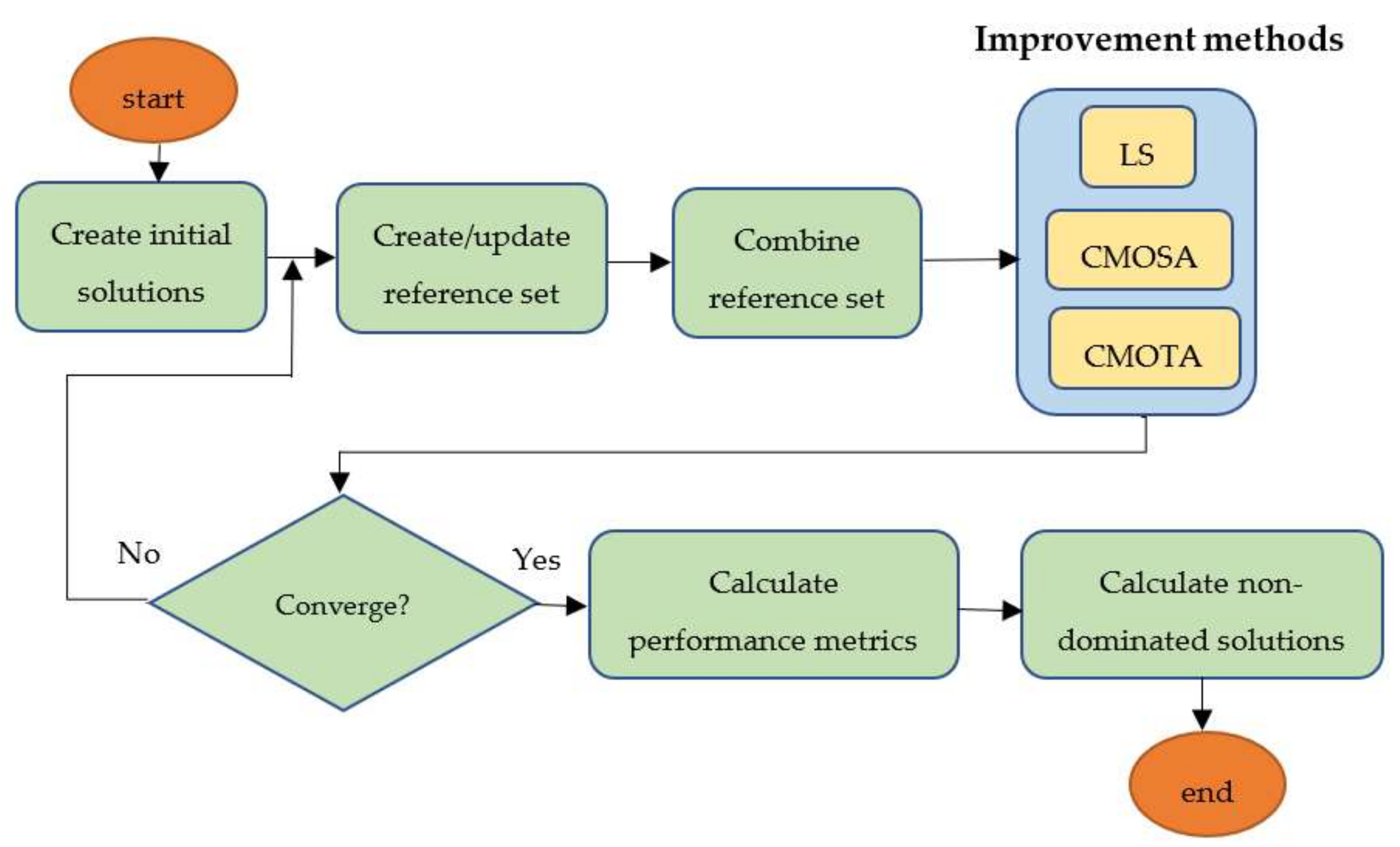
Three hybrid algorithms based on Scatter Search (SS) are proposed for the solution of the MO-JSSP problem. Figure 1 shows the Scatter Search framework showing the three different process which distinguish the three proposed hybrid algorithms.

Figure 1. Scatter Search (SS) Framework.

Algorithm 1 contains the pseudocode of our Scatter Search Algorithm, which is described in detail in the next subsection. Notice that in line five, one of the algorithms CMOSA, CMOTA, or LS can be executed. The goal of Algorithm 1 is to improve the solutions of the reference set.

Algorithm 1. Scatter Search Algorithm
	Input: iterate=0, MAXITERATIONS
	Output: Non-dominated solutions front, metrics values
1:	Generate initial solutions();
2:	while (iterate<=MAXITERATIONS) do
3:	Create/update reference set();
4:	Combine reference set();
5:	Improvement method(); //CMOSA, or CMOTA, or LS algorithm
6:	iterate++
7:	End
8:	Calculate the non-dominate solutions front();
9:	Calculate performance metrics;

4.1. Scatter Search General Framework

Scatter Search (SS) is an algorithm proposed by Glover [10], and it is composed of the following methods:

• Generator of diverse solutions, in which a set P of diverse solutions of size 30 is generated.
• Updater and creator of refSet, from the P solutions, the first three non-dominated and three most diverse are selected, using the Euclidean distance, to form the reference set (RefSet) of size 6.
• Combination of refSet. The six solutions in the refSet are mixed to obtain 30 new solutions. All possible combinations are generated in this process by taking the first half of one solution from the refSet and the second half from another.
• Improvement method. This process tries to improve each new solution created by the combination method. In this work, there are three different improvement methods implemented:
  • A Local Search (LS): consists of performing a set of iterations in which a regular perturbation is applied, which consists in exchanging two operations randomly selected from the current solution to generate a new one. The dominance criterion is applied at each iteration, and the new non-dominated solutions are stored.
  • A Chaotic Threshold Accepting Algorithm (CMOTA). Threshold Accepting (TA) is an algorithm proposed in [33]. In this enhanced method CMOTA, a version adapted to JSSP is used [11].
  • Chaotic Simulated Annealing Algorithm (CMOSA), SA was originally proposed in [34], and in 2021 a new version is implemented under the multiobjective approach [11].

In improvement processes 2) and 3), an analytical tuning process is performed for the algorithm parameters [35]. A regular perturbation is also applied to generate a new solution that is compared to the current one. From the previous comparison, the dominant one is selected, and the non-dominated is discarded. If both are not dominated, one is saved in the set of non-dominated solutions, and the other continues the search. When new non-dominated solutions are not found in both algorithms, a chaotic perturbation is applied. This perturbation consists of using the equation of the logistic maps [36] as a mechanism to escape from stagnation and search diversity in the solutions. A reheating process is also applied, which consists of raising the value of the current temperature parameter to be able to carry out a new scan. The improvement algorithms implemented are described in more detail in the following sections.

4.2. Hybrid Scatter Search with Local Search (SS/LS)

In this algorithm, a Local Search (LS) is applied in the solution improvement phase. Algorithm 2 shows the local search algorithm used. In this algorithm, a set of iterations is performed. In each of them, a regular perturbation is applied to the solution (exchange of two operations) to generate a new one. Dominance is verified between the current solution and the new one created with the perturbation in each iteration. In this verification, three possible cases are generated:

• Case A. If the new solution dominates the current one, then the new solution is saved and replaces the current one to continue the search process.
• Case B. If the current solution dominates the new one, then the new solution is discarded.
• Case C. If the current and the new solution are non-dominated, the current solution is saved, and the new one replaces the current one to continue the search.

4.3. Hybrid Scatter Search with Chaotic Simulated Annealing (SS/CMOSA)

The SS/CMOSA algorithm is based on Chaotic Simulated Annealing Algorithm (CMOSA) [11]. This hybrid algorithm, SS/CMOSA, receives the solutions obtained by a combination process as shown in Figure 1, while CMOSA is shown in Algorithm 3.: one that controls the stop condition and the other internal (Metropolis cycle) that controls the number of iterations carried out for each temperature parameter value.

Algorithm 2. Improvement method: Local Search (LS)
	Input: iterate = 0, MAXITERATIONS
	Output: Current solution, Non-dominated solutions
1:	Current solution = Select one initial solution();
2:	While (iterate ≤ MAXITERATIONS) do
3:	New solution = Perturbation(Current solution);
4:	Calculate makespan, tardiness, flowtime(New solution);
5:	if (New solution dominates Current solution) then
6:	Save(New solution);
7:	Current solution = New solution;
8:	NewSolutionDominatesCurrentSolution = Yes;
9:	end
10:	if (Current solution dominates New solution) then
11:	CurrentSolutionDominatesNewSolution = Yes;
12:	end
13:	if (Current and New solutions are non-dominated) then
14:	Current solution = New solution;
15:	end
16:	iterate++
17:	end

In Algorithm 2, a perturbation is made to the current solution in the internal cycle to generate a new solution. Dominance is verified between the current solution and the new one in each iteration. In this verification, the same three possible previous cases are generated:

• Cases A and C are evaluated similarly to the SS/LS version.
• Case B. According to the Boltzmann probability distribution, when the current solution dominates the new one, the latter could be replaced by the former.

Additionally, a chaotic perturbation and a reheating are applied when stagnation occurs, consisting of a predetermined number of iterations without finding non-dominated solutions. The chaotic perturbation uses the equation of the logistic maps [37], whose main characteristic is that it generates different outputs even in small changes in its input data. Then chaos or chaotic perturbation is a process carried out to restart the search from another point in the space of solutions. Reheating is the process by which the current temperature parameter of the SA algorithm is high; this helps to perform reprocessing that allows reinitializing the search process.

4.4. Hybrid Scatter Search with Chaotic Threshold Accepting (SS/CMOTA)

The Chaotic Threshold Accepting (CMOTA) algorithm is used as an improvement method. In CMOTA (Algorithm 4), there are also two cycles such as CMOSA, one that controls the stop condition (temperature) and the other internal (Metropolis cycle) that controls the number of iterations that are carried out for each value of the temperature parameter.

The same three possible previous cases are generated. Cases A and C are evaluated in the same way as the SS/CMOSA version. In Case B, if the current solution dominates the new solution, the latter can replace the current one in the searching process by using a threshold established in the algorithm.

Similar to CMOSA, this algorithm also applies chaotic perturbation and a reheating process.

Algorithm 3. Improvement method: Chaotic Multi-Objective Simulated Annealing
	Input: iterate = 0, MAXITERATIONS, MAXIMUM ALLOWED STAGNATION SSSSSSTAGNATION
	Output: Current solution, Non-dominated solutions
1:	While (current temperature ≥ final temperature) do
2:	for each Metropolis cycle iteration do
3:	if stagnant = True then
4:	for each local search iteration do
5:	if iteration = 1 then
6:	New solution = chaoticPerturbation(Current solution);
7:	Else
8:	New solution = regularPerturbation(Current solution);
9:	End
10:	if (New solution dominates in all objectives to Current solution) then
11:	Current solution = New solution;
12:	End
13:	End
14:	Else
15:	New solution = regularPerturbation(Current solution);
16:	End
17:	if (New solution ≠ Current solution and it’s not stored in the front) then
18:	if (New solution dominates Current solution) then
19:	Save(New solution);
20:	Current solution = New solution;
21:	NewDominatesCurrent = True;
22:	End
23:	if (Current solution dominates New solution) then
24:	calculates decrement of objective functions;
25:	if (random(0 - 1) < e-decrementCurrenttemperature) then
26:	Save(Current solution);
27:	Current solution = New solution;
28:	CurrentDominatesNew = True;
29:	End
30:	End
31:	if (NewDominatesCurrent = False AND CurrentDominatesNew = False) then
32:	Save(Current solution);
33:	Current solution = New solution;
34:	End
35:	End
36:	End
37:	if (verifyCaught = True) then
38:	if (New solution is dominated by some stored solution) then
39:	stagnant = True;
40:	trappedCounter++;
41:	if (trappedCounter = MAXIMUM ALLOWED STAGNATION) then
42:	verifyCaught = FALSE;
43:	End
44:	End
45:	End
46:	decrease current temperature;
47:	End

Algorithm 4. Improvement method: Chaotic Multi-Objective Threshold Accepting
	Input: iterate = 0, MAXITERATIONS, MAXIMUM ALLOWED STAGNATION SSSSSSTAGNATION
	Output: Current solution, Non-dominated solutions
1:	While (current temperature ≥ final temperature) do
2:	Threshold = current temperature
3:	for each Metropolis cycle iteration do
4:	if stagnant = True then
5:	foreach local search iteration do
6:	if iteration = 1 then
7:	New solution = chaoticPerturbation(Current solution);
8:	else
9:	New solution = regularPerturbation(Current solution);
10:	end
11:	if (New solution dominates in all objectives to Current solution) then
12:	Current solution = New solution;
13:	end
14:	end
15:	else
16:	New solution = regularPerturbation(Current solution);
17:	end
18:	if (New solution ≠ Current solution and it’s not stored in the front) then
19:	if (New solution dominates Current solution) then
20:	Save(New solution);
21:	Current solution = New solution;
22:	NewDominatesCurrent = True;
23:	end
24:	if (Current solution dominates New solution) then
25:	if (random(0 - 1) < Threshold ) then
26:	Save(Current solution);
27:	Current solution = New solution;
28:	CurrentDominatesNew = True;
29:	end
30:	end
31:	if (NewDominatesCurrent = False AND CurrentDominatesNew = False) then
32:	Save(Current solution);
33:	Current solution = New solution;
34:	end
35:	end
36:	end
37:	if (verifyCaught = True) then
38:	if (New solution is dominated by some stored solution) then
39:	stagnant = True;
40:	trappedCounter++;
41:	if (trappedCounter = MAXIMUM ALLOWED STAGNATION) then
42:	verifyCaught = FALSE;
43:	end
44:	end
45:	end
46:	decrease current temperature;
47:	end

5. Computational Experimentation

This section describes the dataset used, the conditions of the experimentation as well as the results obtained.

5.1. Datasets

To perform the experimental evaluation of the algorithm, a benchmark of 70 instances of the problem are used. All the solutions of this dataset have different sizes and degrees of complexity. The instances are divided in six sets:

• Three instances denoted as FT06, FT10, FT20 of Fisher and Thompson [20],
• Ten instances denoted as ORB01–ORB10 of Applegate and Cook [38],
• 40 instances LA01-LA40 presented by Lawrence [39],
• Five instances ABZ5–ABZ9 taken from Baker [37],
• Four instances YN1, YN2, YN3 and YN4 taken from Yamada [40] and,
• Eight instances denoted as TA01, TA11, TA21, TA31, TA41, TA51, TA61, and TA71 taken fromTaillard [41].

The instance sizes of this dataset range from six jobs on six machines (the FT06 instance) to 100 jobs on 20 machines (the instance TA71).

5.2. Experiment Description

Two experiments were carried out with a different number of instances to evaluate the performance of the proposed algorithms.

The first experimentation was carried out with 58 common instances with only three algorithms (IMOEA/D [16], CMOSA, and CMOTA [11]) of the state-of-the-art that used the MID performance metric and the same three objectives. The second experimentation was carried out with 70 instances to compare the results with the CMOSA and CMOTA algorithms proposed in [11]. Each instance was executed 30 times using 30 initial solutions. The set of non-dominated solutions was obtained from the total solutions generated by the 30 executions

The performance metrics used are MID, Spacing, Spread, HV, IGD, Runtime, and the number of non-dominated solutions. Finally, we applied these metrics to the set of non-dominated solutions obtained by the algorithms at the end of their processes.

The execution of the proposed algorithms was carried out in a terminal of the Ehécatl cluster of the Technological Institute of Ciudad Madero, with the following characteristics: Intel^® Xeon^® processor at 2.30 GHz, Memory: 64 Gb (4 × 16 Gb) ddr4-2133, Linux operating system CentOS. C language was used for the implementation, and GCC compiler.

5.3. Comparative Results

Table 2 shows a comparison with the average results obtained by the MID metric for the 58 instances used in the algorithms IMOEA/D [16], CMOSA [11], CMOTA [11], and the proposed SS algorithms. We observed that our hybrid algorithms SS/LS, SS/CMOTA, and SS/CMOSA obtained the best results. Furthermore, the hybrid SS/CMOSA obtained the best result surpassing IMOEA/D by 17%.

Table 2. IMOEA/D, CMOSA, CMOTA, SS/LS, SS/CMOSA, and SS/CMOTA results using MID.

IMOEA/D [16]	CMOSA [11]	CMOTA [11]	SS/LS	SS/CMOSA	SS/CMOTA
18,727.04	15,729.65	16,567.07	15,579.30	15,509.06 *	15,600.19

* Best result obtained.

Table 3 shows the results obtained for each of the 70 instances by the three proposed algorithms, comparing them with the best of the state-of-the-art (CMOSA, CMOTA), taking as a reference the value obtained by the MID metric. The last row shows the average value of the MID metric for each of the algorithms. In this table, we observed that the SS/LS algorithm obtained a better performance since the value of the MID metric is smaller than the other algorithms analyzed.

Table 3. CMOSA, CMOTA, SS/LS, SS/CMOSA, and SS/CMOTA results using MID metric.

	INSTANCE	CMOSA [11]	CMOTA [11]	SS/LS	SS/CMOSA	SS/CMOTA
1	MT06	302.49	302.76	299.01	302.41	303.06
2	MT10	8968.94	9316.19	9514.63	8733.67	8841.43
3	MT05	18,599.1	18,789.48	18,095.69	17,334.15	18,036.81
4	ORB1	9423.07	9707.17	9263.34	9369.55	9400.38
5	ORB2	8129.62	8526.49	8207.86	8175.03	8050.28
6	ORB3	9443.81	9940.47	9618.31	9264.74	9491.26
7	ORB4	9205.69	9874.42	9552.22	9423.15	9407.45
8	ORB5	7983.66	8088.73	8211.05	7836.78	7898.4
9	ORB6	9489.54	9326.38	9639.36	8963.27	8962.67
10	ORB7	3630.48	3758.8	3526.24	3559.64	3605.42
11	ORB8	8268.95	8562.67	8242.37	8222.32	8150.52
12	ORB9	8778.61	9276.51	8872.7	8732.66	8993.75
13	ORB10	8672.67	9001.91	8796.23	8550.83	8568.04
14	LA01	5412.62	5597.42	5467.6	5479.76	5556.06
15	LA02	5031.77	5184.33	5006.39	4961.72	5013.23
16	LA03	4814.76	5134.95	4832.81	4918.78	5018.75
17	LA04	4861.93	5031.3	4929.76	4975.73	4928.21
18	LA05	4562.81	4714.16	4517.06	4555.52	4646.42
19	LA06	10,838.09	10,892.8	10,491.17	10,561.5	10,674.84
20	LA07	10,116.11	10,667.92	9562.58	10,137.43	10,186.86
21	LA08	10,042.56	10,009.01	9698.32	9896.07	10,389.5
22	LA09	11,036.3	11,411.96	10,893.66	10,861.87	11,408.09
23	LA10	11,202.9	11,365.93	10,898.95	11,333.39	11,302.51
24	LA11	19,027.38	19,802.15	17,161.79	19,450.04	19,350.97
25	LA12	15,911.86	16,330.94	14,623.73	15,892.3	15,600.23
26	LA13	17,928.81	18,139.11	17,160.73	17,743.58	17,990.65
27	LA14	20,538.67	20,433.48	18,234.8	20,062.12	20,181.51
28	LA15	19,316.53	20,217.82	18,501.01	19,201.56	19,108.72
29	LA16	8471.45	8504.98	8637.69	8250.89	8386.26
30	LA17	7360.64	7642.17	7393.33	7443.46	7349.59
31	LA18	7799.15	7970.16	7892.52	7762.4	7722.94
32	LA19	7886.52	8018.64	7928.09	7560.93	7822.05
33	LA20	8223.4	8504.94	8061.01	7976.07	8075.83
34	LA21	14,660.24	15,048.78	14,705	14,496.21	14,452.81
35	LA22	13,791.82	14,273.02	13,431.25	13,289.3	13,582.21
36	LA23	14,332.13	14,681.08	14,610.65	14,165.27	13,828.52
37	LA24	13,621.56	14,220.91	13,997.19	13,458.13	13,717.81
38	LA25	14,072.76	14,339.68	14,544.46	13,879.81	14,077.29
39	LA26	23,328.49	23,931.83	24,030.06	23,029.41	22,900.82
40	LA27	23,562.7	24,858.52	24,299.39	23,400.87	23,281.32
41	LA28	23,470.98	24,011.52	23,280.26	23,310.77	23,219.81
42	LA29	23,693.39	24,403.19	23,474.51	22,460.64	22,681.31
43	LA30	25,644.07	25,928.94	23,662.84	24,696.12	25,366.63
44	LA31	47,688.21	49,005.79	47,177.36	47,865.09	48,915.77
45	LA32	49,824.88	51,503.92	49,501.67	49,915.58	49,907.61
46	LA33	45,505.39	48,241.29	46,761.86	45,943.56	46,155.67
47	LA34	48,515.97	50,594.96	48,225.35	48,105.61	48,159.25
48	LA35	51,334.25	52,684.38	49,499.12	50,174.39	49,983.62
49	LA36	20,064.09	20,496.35	20,810.13	18,924.07	19,294.57
50	LA37	20,914.82	21,563.64	19,795.94	20,609.68	20,459.21
51	LA38	18,259.69	18,899.71	19,528.82	17,574.33	17,824.86
52	LA39	18,883.47	19,664.49	17,721.37	18,043.34	17,564.64
53	LA40	18,713.13	19,548.43	18,973.49	18,204.15	18,239.15
54	ABZ5	11,065.38	11,716.44	11,455.08	11,263.35	11,153.71
55	ABZ6	8562.26	8777.87	8547.61	8417.55	8412.77
56	ABZ7	13,456.23	14,117.93	13,666.34	13,533.63	13,433.57
57	ABZ8	13,876.7	14,964.84	13,829.45	13,659.58	13,917.87
58	ABZ9	14,196.03	14,482.01	14,338.05	13,611.68	13,857.5
59	YN01	19,600.96	19,081.94	18,852.58	18,614.34	18,513.43
60	YN02	19,478.97	29,387.6	20,381.93	18,911.92	19,185.31
61	YN03	19,373.68	37,958.48	19,617.2	18,652.67	18,646.75
62	YN04	20,795.84	20,085.05	20,537.93	20,019.8	20,302.96
63	TA01	18,854.25	21,077.84	17,900.21	18,028.25	18,372.28
64	TA11	28,456.37	19,829.68	27,650.77	27,426.51	26,732.44
65	TA21	36,784.31	21,706.29	38,361.95	35,354.63	35,020.33
66	TA31	57,276.28	58,910.97	55,016.34	51,624.54	55,253.5
67	TA41	67,727.19	70,740.02	65,540.4	66,060.72	67,477.21
68	TA51	149,060.96	147,166.01	142,621.68	145,129.97	140,875.79
69	TA61	163,794.79	165,040.63	157,115.67	156,896.57	159,441.06
70	TA71	634,090.21	633,330.29	593,742.24	614,082.8	604,620.66
AVG		30,680.19	31,233.15	29,727.69 *	29,861.83	29,846.47

* Best result obtained.

Table 4 summarizes the experiment results with 70 instances and five metrics; it contains the average values obtained by executing the algorithms 30 times. The first column has the name of the evaluated metric. The next two columns show the results of the two best state-of-the-art algorithms (CMOSA and CMOTA). Finally, the last three columns show the results for the three hybrid proposed algorithms (SS/LS, SS/CMOSA, and SS/CMOTA).

Table 4. Comparison of CMOSA, CMOTA and SS/LS, SS/CMOSA and SS/CMOTA results.

Metric	CMOSA [11]	CMOTA [11]	SS/LS	SS/CMOSA	SS/CMOTA
MID	30,680.19	31,233.15	29,727.69 *	29,861.83	29,846.47
Spacing	28,445.62	28,183.17	27,345.38	26,466.71	26,168.68 *
HV	0.42	0.42	0.42	0.42	0.44 *
Spread	24,969.31	23,401.88	23,935.95	20,961.48 *	21,307.87
IGD	1666.25	1870.94	1381.14 *	1449.77	1433.89
Runtime	495.22	229.42	133.65 *	1220.47	1202.18
Number of solutions	10.57 *	8.66	9.51	8.63	8.56

* Best result obtained.

In Table 4, the best values are highlighted and marked with an asterisk (*). An approximate Pareto front is used in the case of metrics in which it is necessary to use a True Pareto front [24]. The approximate Pareto front is generated by previous executions of developed algorithms throughout the study of this problem.

We can observe that SS/LS obtains the best result for MID and IGD metrics. This algorithm uses the shortest processing time, which means that it has the best convergence and generates the highest number of non-dominated solutions of the three proposed hybrid algorithms. The results indicate that the solutions found by SS/LS are closer to the origin point (0,0,0); they are closer on average to the approximate front and were achieved with the lowest amount of execution time. SS/CMOSA algorithm obtains the best Spread, which means that the generated solutions are very well distributed on the non-dominated solutions front. On the other hand, SS/CMOTA achieved the best Spacing and HV values, which indicate that this algorithm- has a more uniform Spacing and the best solution space coverage. In other words, the hybrid algorithms proposed in this paper obtained the best results for these datasets.

Finally, the non-dominated solution fronts obtained by the proposed algorithms for the 70 instances are included in Appendix A.

6. Conclusions

This paper presents three Hybrid Multi-Objective algorithms for JSSP, named SS/LS, SS/CMOSA, and SS/CMOTA. Three objectives are considered: makespan, total tardiness, and total flow time. Furthermore, we present an experimental evaluation applying six performance metrics.

Regarding the results from the comparison, we observe that SS/LS generates solutions closer to the origin point and PF_approx. It provides more solutions than the others’ algorithms and uses the minimum runtime. SS/CMOSA generates solutions with a better distribution concerning PF_approx. Furthermore, SS/CMOTA generates better-distributed solutions in the PF_calc and better coverage, as shown by the HV metric. The results obtained by the proposed algorithms SS/LS, SS/CMOSA, and SS/CMOTA compared with some of the best algorithms in the literature show that they are among the best in the area. We highlight that our proposed SS/LS algorithm reduces processing time by 43% compared to the fastest in the state-of-the-art.

References

- Garey, M.R.; Johnson, D.S.; Sethi, R. PageRank: The complexity of flowshop and jobshop scheduling. Math. Oper. Res. 1976, 1, 117–129. [Google Scholar] [CrossRef] [Scilit]
- Pinedo, M. Scheduling Theory Algorithm, and Systems, 5th ed.; Springer: Berlin/Heidelberg, Germany; New York, NY, USA, 2016; ISBN 978-3-319-26578-0. [Google Scholar]
- Yang, Y.B. Methods and Techniques Used for Job Shop Scheduling, MSc. Research Project, Florida Technological University. 1972. Available online: https://stars.library.ucf.edu/cgi/viewcontent.cgi?article=1389&context=rtd (accessed on 29 November 2021).
- Xing, L.N.; Chen, Y.W.; Yang, K.W. Multi-objective flexible job shop schedule: Design and evaluation by simulation modeling. Appl. Soft Comput. 2009, 9, 362–376. [Google Scholar] [CrossRef] [Scilit]
- Yuan, Y.; Xu, H. Multiobjective flexible job shop scheduling using memetic algorithms. IEEE Trans. Autom. Sci. Eng. 2015, 12, 336–353. [Google Scholar] [CrossRef] [Scilit]
- Kaplanoglu, V. An object-oriented approach for multi-objective flexible job-shop scheduling problem. Expert Syst. Appl. 2016, 45, 71–84. [Google Scholar] [CrossRef] [Scilit]
- Bao, Q.; Soubeyran, A. Variational principles in set optimization with domination structures and application to changing jobs. J. Appl. Numer. Optim. 2019, 1, 217–241. [Google Scholar]
- Luu, D.V.; Linh, P.T. Optimality and duality for nonsmooth multiobjective fractional problems using convexificators. J. Nonlinear Funct. Anal. 2021, 2021, 1. [Google Scholar]
- Pereira, O.; Júnior, V.L.d.; Soubeyran, A. Inexact Multi-Objective Local Search Proximal Algorithms: Application to Group Dynamic and Distributive Justice. J. Optim. Theory Appl. 2018, 177, 181–200. [Google Scholar]
- Glover, F. Heuristics for integer programming using surrogate constraints. Decis. Sci. 1977, 8, 156–166. [Google Scholar] [CrossRef] [Scilit]
- Frausto-Solis, J.; Hernández-Ramírez, L.; Castilla-Valdez, G.; González-Barbosa, J.; Sánchez, J. Chaotic multi-objective simulated annealing and threshold accepting for job shop scheduling problem. Math. Comput. Appl. 2021, 26, 8. [Google Scholar] [CrossRef] [Scilit]
- Suresh, R.K.; Mohanasundaram, M. Pareto archived simulated annealing for job shop scheduling with multiple objectives. Int. J. Adv. Manuf. Technol. 2006, 29, 184–196. [Google Scholar] [CrossRef] [Scilit]
- Bandyopadhyay, S.; Saha, S.; Maulik, U.; Deb, K. A Simulated Annealing-Based Multiobjective Optimization Algorithm: AMOSA. Evol. Comput. IEEE Trans. 2008, 12, 269–283. [Google Scholar] [CrossRef] [Scilit]
- Deb, K.; Agrawal, S.; Pratap, A.; Meyarivan, T. A fast elitist non-dominated sorting genetic algorithm for multiobjective optimization: NSGA-II. In International Conference on Parallel Problem Solving from Nature; Spring: Berlin/Heidelberg, Germany, 2000; Volume 1917. [Google Scholar]
- Kachitvichyanukul, V.; Sitthitham, S. A two-stage genetic algorithm for multiobjective job shop scheduling problems. J. Intell. Manuf. 2009, 22, 355–365. [Google Scholar] [CrossRef] [Scilit]
- Zhao, F.; Chen, Z.; Wang, J.; Zhang, C. An improved MOEA/D for multiobjective job shop scheduling problem. Int. J. Comput. Integr. Manuf. 2016, 30, 616–640. [Google Scholar] [CrossRef] [Scilit]
- Zitzler, E.; Deb, K.; Thiele, L. Comparison of Multiobjective Evolutionary Algorithms: Empirical Results. Evol. Comput. 2000, 8, 173–195. [Google Scholar] [CrossRef] [Scilit]
- Karimi, N.; Zandieh, M.; Karamooz, H. Bi-objective group scheduling in hybrid flexible flowshop: A multi-phase approach. Expert Syst. Appl. 2010, 37, 4024–4032. [Google Scholar] [CrossRef] [Scilit]
- González, M.; Oddi, A.; Rasconi, R. Multiobjective optimization in a job shop with energy costs through hybrid evolutionary techniques. In Proceedings of the Twenty-Seventh International Conference on Automated Planning and Scheduling, Pittsburgh, PA, USA, 18–23 June 2017; pp. 140–148. [Google Scholar]
- Fisher, H.; Thompson, G.L. Probabilistic learning combinations of local job-shop scheduling rules. Ind. Sched. 1963, 1, 225–251. [Google Scholar]
- Méndez-Hernández, B.; Rodriguez Bazan, E.D.; Martinez, Y.; Libin, P.; Nowe, A. A Multiobjective Reinforcement Learning Algorithm for JSSP. In Proceedings of the 28th International Conference on Artificial Neural Networks, Munich, Germany, 17–19 September 2019; pp. 567–584. [Google Scholar] [CrossRef] [Scilit]
- Zhang, J.; Ding, G.; Zou, Y.; Qin, S.; Fu, J. Review of job shop scheduling research and its new perspectives under Industry 4.0. J. Intell. Manuf. 2019, 30, 1809–1830. [Google Scholar] [CrossRef] [Scilit]
- Deb, K. Multiobjective Optimization Using Evolutionary Algorithms; Wiley: New York, NY, USA, 2001. [Google Scholar]
- Coello, C.; Veldhuizen, D.; Lamont, G. Evolutionary Algorithms for Solving Multiobjective Problems, 2nd ed.; Springer: Berlin, Germany, 2007; ISBN 978-0-387-36797-2. [Google Scholar]
- Okabe, T.; Jin, Y.; Sendhoff, B. A critical survey of performance indices for multiobjective optimisation. In Proceedings of the 2003 Congress on Evolutionary Computation, 2003. CEC ’03, Canberra, ACT, Australia, 8–12 December 2003; IEEE: Piscataway, NJ, USA, 2003; Volume 2, pp. 878–885. [Google Scholar]
- Schott, J.R. Fault Tolerant Design Using Single and Multicriteria Genetic Algorithm Optimization. Master’s Thesis, Department of Aeronautics and Astronautics, Massachusetts Institute of Technology, Cambridge, MA, USA, 1995. [Google Scholar]
- Veldhuizen, D.A.V. Multiobjective Evolutionary Algorithms: Classifications, Analyses, and New Innovations. Ph.D. Thesis, Air Force Institute of Technology, Wright-Patterson AFB, Dayton, OH, USA, 1999. [Google Scholar]
- Coello, C.; Cruz, N. Solving Multiobjective Optimization Problems Using an Artificial Immune System. Genet. Program. Evolvable Mach. 2005, 6, 163–190. [Google Scholar] [CrossRef] [Scilit]
- Sawaragi, Y.; Nakagama, H.; Tanino, T. Theory of Multiobjective Optimization; Springer: Boston, MA, USA, 1985. [Google Scholar]
- Bakuli, D.L. A Survey of Multiobjective Scheduling Techniques Applied to the Job Shop Problem (JSP). In Applications of Management Science: In Productivity, Finance, and Operations; Emerald Group Publishing Limited: Bingley, UK, 2015; pp. 51–62. [Google Scholar]
- Baker, K.R. Sequencing rules and due-date assignments in job shop. Manag. Sci. 1984, 30, 1093–1104. [Google Scholar] [CrossRef] [Scilit]
- Yazid, M.; Dauzère-Pérès, S.; Chams, L. A general approach for optimizing regular criteria in the job-shop scheduling problem. Eur. J. Oper. Res. 2011, 212, 33–42. [Google Scholar] [CrossRef] [Scilit]
- Dueck, G.; Scheuer, T. Threshold Accepting: A General Purpose Algorithm Appearing Superior to Simulated Annealing. J. Comput. Phys. 1990, 90, 161–175. [Google Scholar] [CrossRef] [Scilit]
- Kirkpatrick, S.; Gelatt, C.D.; Vecchi, M.P. Optimization by simulated annealing. Am. Assoc. Adv. Sci. 1983, 220, 671–680. [Google Scholar]
- Sanvicente, S.H.; Frausto, J. A method to establish the cooling scheme in simulated annealing like algorithms. In Proceedings of the International Conference on Computational Science and Its Applications, Assisi, Italy, 14–17 May 2004; pp. 755–763. [Google Scholar]
- May, R. Simple Mathematical Models with Very Complicated Dynamics. Nature 1976, 26, 457. [Google Scholar] [CrossRef] [Scilit]
- Adams, J.; Balas, E.; Zawack, D. The shifting bottleneck procedure for job shop scheduling. Manag. Sci. 1988, 34, 391–401. [Google Scholar] [CrossRef] [Scilit]
- Applegate, D.; Cook, W. A computational study of the job-shop scheduling problem. ORSA J. Comput. 1991, 3, 149–156. [Google Scholar] [CrossRef] [Scilit]
- Lawrence, S. Resource Constrained Project Scheduling: An Experimental Investigation of Heuristic Scheduling Techniques (Supplement); Graduate School of Industrial Administration, Carnegie-Mellon University: Pittsburgh, PA, USA, 1984. [Google Scholar]
- Yamada, T.; Nakano, R. A genetic algorithm applicable to large-scale job-shop problems. In Proceedings of the Second International Conference on Parallel Problem Solving from Nature, Brussels, Belgium, 28–30 September1992; pp. 281–290. [Google Scholar]
- Taillard, E. Benchmarks for basic scheduling problems. Eur. J. Oper. Res. 1993, 64, 278–285. [Google Scholar] [CrossRef] [Scilit]
Publisher’s Note: MDPI stays neutral with regard to jurisdictional claims in published maps and institutional affiliations. |
© 2022 by the authors. Licensee MDPI, Basel, Switzerland. This article is an open access article distributed under the terms and conditions of the Creative Commons Attribution (CC BY) license (https://creativecommons.org/licenses/by/4.0/).