Solution to Integral Equation in an O-Complete Branciari b-Metric Spaces

Abstract

In this paper, we prove fixed point theorem via orthogonal Geraghty type $\alpha$-admissible contraction map in an orthogonal complete Branciari b-metric spaces context. An example is presented to strengthen our main result. We provided an application to find the existence and uniqueness of a solution to the Volterra integral equation. We have compared the approximate solution and exact solution numerically.

1. Introduction

In 1922, Banach initiated the famous fixed point result called Banach contraction principle. This is one of the most important and fundamental results in complete metric space. The generalization of b-metric space was introduced by Bakhtin and Czerwik [1,2]. It is the most widely applied fixed point result in many branches of Mathematics and Sciences. A number of authors have defined contractive type mappings on b-metric spaces in many different directions to improve the results see [3,4,5,6,7,8,9]. The concept of Branciari metric space was initiated by Branciari [10] in 2000. In 2015, George et al. [11] introduced the generalization of Branciari b-metric spaces and proved some fixed point results. Thereafter, many authors initiated and extended the results of Branciari metric spaces and Branciari b-metric spaces and proved fixed point theorems in such spaces, see [12,13] and the references therein.

In 1973, one of the interesting results was given by Geraghty [14] in the setting of complete metric spaces by considering an auxiliary function. Several papers have been improved to the Geraghty contraction mapping type of fixed point theory in complete b-metric spaces refers to see [15,16,17]. Very recently, Samet et al. [18] initiated $\alpha$-admissible mapping and also proved the fixed results for $\alpha$-$\psi$-contractive mappings. Tunç et al. [19,20] proved the existence of solutions of some fixed results of non-linear 2D integral equations and also found the stability, integrability and boundedness of systems of integro-differential equations. In 2017, Eshaghi Gordji et al. [21] has established the main idea of the orthogonality and framework to our main finding of results. And also, Eshaghi Gordji and Habibi [22] has extended and proved some fixed point theorem in generalized O-metric spaces. For other results related to orthogonal concepts, see [23,24,25,26,27,28,29,30].

In this paper, we introduce the fixed point theorem for an O-generalized O-Geraghty type $\alpha$-admissible (in short, O-G-$\alpha$ admissible) mapping on O-complete Branciari b-metric space and also we presented an example and application to integral equation by using our main results.

2. Preliminaries

We recall the following definitions and results will be needed in the sequel.

The notion of b-metric space was introduced by Bakhtin [1] in 1989, as follows:

Definition 1

([1]). Let $\mathcal{V}$ be a non-void set and a constant $\delta \ge 1$. A function ${\mathfrak{w}}_{\mathfrak{b}}:\mathcal{V}\times \mathcal{V}⟶{\mathbb{R}}^{+}$ is called a b-metric if the below axioms hold, for all $\mathfrak{s},\upsilon ,\vartheta \in \mathcal{V}$:

$\left(A_1\right)$

${\mathfrak{w}}_{\mathfrak{b}}(\mathfrak{s},\upsilon )=0$ if and only if $\mathfrak{s}=\upsilon$,

$\left(A_2\right)$

${\mathfrak{w}}_{\mathfrak{b}}(\mathfrak{s},\upsilon )={\mathfrak{w}}_{\mathfrak{b}}(\upsilon ,\mathfrak{s})$,

$\left(A_3\right)$

${\mathfrak{w}}_{\mathfrak{b}}(\mathfrak{s},\upsilon )\le \delta [{\mathfrak{w}}_{\mathfrak{b}}(\mathfrak{s},\vartheta )+{\mathfrak{w}}_{\mathfrak{b}}(\vartheta ,\upsilon )]$.

• The pair $(\mathcal{V},{\mathfrak{w}}_{\mathfrak{b}})$ is said to be a b-metric space with constant $\delta \ge 1$.

Example 1.

Let $(\mathcal{V},{\mathfrak{w}}_{\mathfrak{b}})$ be a metric space and let $\gamma >1$, $E\ge 0$ and $L>0$. For $\mathfrak{s},\upsilon \in \mathcal{V}$, set $P(\mathfrak{s},\upsilon )=E{\mathfrak{w}}_{\mathfrak{b}}(\mathfrak{s},\upsilon )+L{\mathfrak{w}}_{\mathfrak{b}}{(\mathfrak{s},\upsilon )}^{\gamma }$. Then $(\mathcal{V},{\mathfrak{w}}_{\mathfrak{b}})$ is a b-metric space with the parameter $\delta =2^{\gamma -1}$ and not a metric space on $\mathcal{V}$.

Branciari [10] initiated the concept of Branciari metric space as follows:

Definition 2

([10]). Let $\mathcal{V}$ be a non void set. A function ${\mathfrak{w}}_{\mathfrak{b}}:\mathcal{V}\times \mathcal{V}⟶{\mathbb{R}}^{+}$ is called a Branciari metric if the below axioms hold, for all $\mathfrak{s},\upsilon \in \mathcal{V}$:

$\left(B_1\right)$

${\mathfrak{w}}_{\mathfrak{b}}(\mathfrak{s},\upsilon )=0$ if and only if $\mathfrak{s}=\upsilon$,

$\left(B_2\right)$

${\mathfrak{w}}_{\mathfrak{b}}(\mathfrak{s},\upsilon )={\mathfrak{w}}_{\mathfrak{b}}(\upsilon ,\mathfrak{s})$,

$\left(B_3\right)$

${\mathfrak{w}}_{\mathfrak{b}}(\mathfrak{s},\upsilon )\le {\mathfrak{w}}_{\mathfrak{b}}(\mathfrak{s},\omega )+{\mathfrak{w}}_{\mathfrak{b}}(\omega ,\mu )+{\mathfrak{w}}_{\mathfrak{b}}(\mu ,\upsilon )$ for all distinct points $\omega ,\mu \in \mathcal{V}/\{\mathfrak{s},\upsilon \}$.

• The pair $(\mathcal{V},{\mathfrak{w}}_{\mathfrak{b}})$ is said to be a Branciari metric space (in short, BMS).

The notion of Branciari b-metric space was initiated by George [11] as follows:

Definition 3

([11]). Let $\mathcal{V}$ be a non void set and a constant $\delta \ge 1$. A function ${\mathfrak{w}}_{\mathfrak{b}}:\mathcal{V}\times \mathcal{V}⟶{\mathbb{R}}^{+}$ is said to be a Branciari b-metric if the below axioms hold, for all $\mathfrak{s},\upsilon \in \mathcal{V}$:

$\left(B_1\right)$

${\mathfrak{w}}_{\mathfrak{b}}(\mathfrak{s},\upsilon )=0$ if and only if $\mathfrak{s}=\upsilon$,

$\left(B_2\right)$

${\mathfrak{w}}_{\mathfrak{b}}(\mathfrak{s},\upsilon )={\mathfrak{w}}_{\mathfrak{b}}(\upsilon ,\mathfrak{s})$,

$\left(B_3\right)$

${\mathfrak{w}}_{\mathfrak{b}}(\mathfrak{s},\upsilon )\le \delta [{\mathfrak{w}}_{\mathfrak{b}}(\mathfrak{s},\omega )+{\mathfrak{w}}_{\mathfrak{b}}(\omega ,\mu )+{\mathfrak{w}}_{\mathfrak{b}}(\mu ,\upsilon )]$ for all distinct points $\omega ,\mu \in \mathcal{V}/\{\mathfrak{s},\upsilon \}$.

• Then, the pair $(\mathcal{V},{\mathfrak{w}}_{\mathfrak{b}})$ is said to be a Branciari b-metric space (in short, $B_{b}MS$).

The following proposition was proved by Erhan [13].

Proposition 1

([13]). Let $\left\{{\mathfrak{s}}_{\widehat{ı}}\right\}$ be a Cauchy sequence in a $BMS$ $(\mathcal{V},{\mathfrak{w}}_{\mathfrak{b}})$ such that ${lim}_{\widehat{ı}\to \infty }{\mathfrak{w}}_{\mathfrak{b}}({\mathfrak{s}}_{\widehat{ı}},\upsilon )=0$, where $\mathfrak{s}\in \mathcal{V}$. Then

$$\begin{array}{c}\hfill \underset{\widehat{ı}\to \infty }{lim}{\mathfrak{w}}_{\mathfrak{b}}({\mathfrak{s}}_{\widehat{ı}},\upsilon )={\mathfrak{w}}_{\mathfrak{b}}(\mathfrak{s},\upsilon ),forall\upsilon \in \mathcal{V}.\end{array}$$

In particular, the $\left\{{\mathfrak{s}}_{\widehat{ı}}\right\}$ does not converge to υ if $\mathfrak{s}\ne \upsilon$.

Geraghty [14] introduced the Geraghty type contraction mappings who have extended the results for Banach contraction theorem by the property defined as the set of all functions $\alpha :{\mathbb{R}}^{+}\to [0,1)$ satisfying the condition:

$$\begin{array}{c}\hfill \underset{\widehat{ı}\to \infty }{lim}\alpha \left({\varrho }_{\widehat{ı}}\right)=1\mathrm{implies}\underset{\widehat{ı}\to \infty }{lim}{\varrho }_{\widehat{ı}}=0.\end{array}$$

Theorem 1

([14]). Let $(\mathcal{V},{\mathfrak{w}}_{\mathfrak{b}})$ be a complete metric space and a mapping $\mathfrak{P}:\mathcal{V}\to \mathcal{V}$ is satisfying the following:

$$\begin{array}{c}\hfill {\mathfrak{w}}_{\mathfrak{b}}(\mathfrak{P}\mathfrak{s},\mathfrak{P}\upsilon )\le \gamma \left({\mathfrak{w}}_{\mathfrak{b}}(\mathfrak{s},\upsilon )\right){\mathfrak{w}}_{\mathfrak{b}}(\mathfrak{s},\upsilon ),\forall \mathfrak{s},\upsilon \in \mathcal{V},\end{array}$$

where $\gamma \in {\mathcal{F}}_{\delta }$. Then $\mathfrak{P}$ has a UFP (Briefly unique fixed point).

Dukic et al. [15] reconsidered the above Theorem 1 for the framework of b-metric spaces in 2011.

Consider a b-metric space $(\mathcal{V},{\mathfrak{w}}_{\mathfrak{b}})$ with constant $\delta \ge 1$ and the set ${\mathcal{F}}_{\delta }$ of all functions $\gamma :{\mathbb{R}}^{+}\to [0,\frac{1}{\delta })$, satisfying the condition:

$$\begin{array}{c}\hfill \underset{\widehat{ı}\to \infty }{lim}\gamma \left({\varrho }_{\widehat{ı}}\right)=\frac{1}{\delta }\Rightarrow \underset{\widehat{ı}\to \infty }{lim}{\varrho }_{\widehat{ı}}=0.\end{array}$$

(1)

Theorem 2

([15]). Let $(\mathcal{V},{\mathfrak{w}}_{\mathfrak{b}})$ be a complete b-metric space with constant $\delta \ge 1$ and $\mathfrak{P}:\mathcal{V}\to \mathcal{V}$ be a self-map. Suppose that there exists $\gamma \in {\mathcal{F}}_{\delta }$ such that,

$$\begin{array}{c}\hfill {\mathfrak{w}}_{\mathfrak{b}}(\mathfrak{P}\mathfrak{s},\mathfrak{P}\upsilon )\le \gamma \left({\mathfrak{w}}_{\mathfrak{b}}(\mathfrak{s},\upsilon )\right){\mathfrak{w}}_{\mathfrak{b}}(\mathfrak{s},\upsilon )\end{array}$$

for all $\mathfrak{s},\upsilon \in \mathcal{V}$. Then $\mathfrak{P}$ has a UFP ${\mathfrak{s}}_0\in \mathcal{V}$.

Remark 1

([15]). If we replace $BMS$ by $B_{b}MS$, then proposition (1) holds.

Definition 4

([15]). A mapping $\mathfrak{P}:\mathcal{V}\to \mathcal{V}$ is called α-admissible if for all $\mathfrak{s},\upsilon \in \mathcal{V}$ we have

$$\begin{array}{c}\hfill \alpha (\mathfrak{s},\upsilon )\ge 1\Rightarrow \alpha (\mathfrak{P}\mathfrak{s},\mathfrak{P}\upsilon )\ge 1,\end{array}$$

where $\alpha :\mathcal{V}\times \mathcal{V}\to {\mathbb{R}}^{+}$ is a given function.

Definition 5

([15]). Let $(\mathcal{V},{\mathfrak{w}}_{\mathfrak{b}})$ be a $B_{b}MS$ with a parameter $\delta \ge 1$ and let $\alpha :\mathcal{V}\times \mathcal{V}\to {\mathbb{R}}^{+}$ and $\gamma \in {\mathcal{F}}_{\delta }$ be two functions. A generalized Geraghty type α-admissible (in short, $G\text{-}\alpha$-admissible) contractive mapping $\mathfrak{P}:\mathcal{V}\to \mathcal{V}$ is of type-(1) if it is α-admissible and the following condition holds

$$\begin{array}{c}\hfill \alpha (\mathfrak{s},\upsilon ){\mathfrak{w}}_{\mathfrak{b}}(\mathfrak{P}\mathfrak{s},\mathfrak{P}\upsilon )\le \gamma \left(\mathcal{K}(\mathfrak{s},\upsilon )\right)\mathcal{K}(\mathfrak{s},\upsilon ),\forall \mathfrak{s},\upsilon \in \mathcal{V},\end{array}$$

where

$$\begin{array}{c}\hfill \mathcal{K}(\mathfrak{s},\upsilon )=max\{{\mathfrak{w}}_{\mathfrak{b}}(\mathfrak{s},\upsilon ),{\mathfrak{w}}_{\mathfrak{b}}(\mathfrak{s},\mathfrak{P}\mathfrak{s}),{\mathfrak{w}}_{\mathfrak{b}}(\upsilon ,\mathfrak{P}\upsilon )\}.\end{array}$$

Theorem 3

([15]). Let $(\mathcal{V},{\mathfrak{w}}_{\mathfrak{b}})$ be a $B_{b}MS$ with a parameter $\delta \ge 1$ and let $\alpha :\mathcal{V}\times \mathcal{V}\to {\mathbb{R}}^{+}$ and $\gamma \in {\mathcal{F}}_{\delta }$ be two functions. Let $\mathfrak{P}:\mathcal{V}\to \mathcal{V}$ be an α-admissible mapping satisfying

$$\begin{array}{c}\hfill \alpha (\mathfrak{s},\upsilon ){\mathfrak{w}}_{\mathfrak{b}}(\mathfrak{P}\mathfrak{s},\mathfrak{P}\upsilon )\le \gamma \left(\mathcal{K}(\mathfrak{s},\upsilon )\right)\mathcal{K}(\mathfrak{s},\upsilon ),\forall \mathfrak{s},\upsilon \in \mathcal{V},\end{array}$$

(2)

where

$$\begin{array}{c}\hfill \mathcal{K}(\mathfrak{s},\upsilon )=max\{{\mathfrak{w}}_{\mathfrak{b}}(\mathfrak{s},\upsilon ),{\mathfrak{w}}_{\mathfrak{b}}(\mathfrak{s},\mathfrak{P}\mathfrak{s}),{\mathfrak{w}}_{\mathfrak{b}}(\upsilon ,\mathfrak{P}\upsilon )\}.\end{array}$$

Then $\mathfrak{P}$ has a UFP.

We next define the Geraghty type mappings of another class on $B_{b}MS$.

Definition 6

([15]). Let $(\mathcal{V},{\mathfrak{w}}_{\mathfrak{b}})$ be a $B_{b}MS$ with a parameter $\delta \ge 1$ and let $\alpha :\mathcal{V}\times \mathcal{V}\to {\mathbb{R}}^{+}$ and $\gamma \in {\mathcal{F}}_{\delta }$ be two functions. Then a $G\text{-}\alpha$-admissible contractive mapping $\mathfrak{P}:\mathcal{V}\to \mathcal{V}$ is of type-(2) if it is α-admissible and the following condition holds

$$\begin{array}{c}\hfill \alpha (\mathfrak{s},\upsilon ){\mathfrak{w}}_{\mathfrak{b}}(\mathfrak{P}\mathfrak{s},\mathfrak{P}\upsilon )\le \gamma \left(\mathcal{N}(\mathfrak{s},\upsilon )\right)\mathcal{N}(\mathfrak{s},\upsilon ),\forall \mathfrak{s},\upsilon \in \mathcal{V},\end{array}$$

where

$$\begin{array}{c}\hfill \mathcal{N}(\mathfrak{s},\upsilon )=max\{{\mathfrak{w}}_{\mathfrak{b}}(\mathfrak{s},\upsilon ),\frac{1}{2}[{\mathfrak{w}}_{\mathfrak{b}}(\mathfrak{s},\mathfrak{P}\mathfrak{s}),{\mathfrak{w}}_{\mathfrak{b}}(\upsilon ,\mathfrak{P}\upsilon )]\}.\end{array}$$

Remark 2

([15]). For all $\mathfrak{s},\upsilon \in \mathcal{V}$ the relation ${\mathfrak{w}}_{\mathfrak{b}}(\mathfrak{s},\upsilon )\le \mathcal{N}(\mathfrak{s},\upsilon ))\le \mathcal{K}(\mathfrak{s},\upsilon )$ holds.

Theorem 4

([15]). Let $(\mathcal{V},{\mathfrak{w}}_{\mathfrak{b}})$ be a $B_{b}MS$ with a parameter $\delta \ge 1$ and let $\alpha :\mathcal{V}\times \mathcal{V}\to {\mathbb{R}}^{+}$ and $\gamma \in {\mathcal{F}}_{\delta }$ be two functions. Let $\mathfrak{P}:\mathcal{V}\to \mathcal{V}$ be an α-admissible mapping satisfying

$$\begin{array}{c}\hfill \alpha (\mathfrak{s},\upsilon ){\mathfrak{w}}_{\mathfrak{b}}(\mathfrak{P}\mathfrak{s},\mathfrak{P}\upsilon )\le \gamma \left(\mathcal{N}(\mathfrak{s},\upsilon )\right)\mathcal{N}(\mathfrak{s},\upsilon ),\forall \mathfrak{s},\upsilon \in \mathcal{V},\end{array}$$

where

$$\begin{array}{c}\hfill \mathcal{N}(\mathfrak{s},\upsilon )=max\{{\mathfrak{w}}_{\mathfrak{b}}(\mathfrak{s},\upsilon ),\frac{1}{2}[{\mathfrak{w}}_{\mathfrak{b}}(\mathfrak{s},\mathfrak{P}\mathfrak{s}),{\mathfrak{w}}_{\mathfrak{b}}(\upsilon ,\mathfrak{P}\upsilon )]\}.\end{array}$$

Then, $\mathfrak{P}$ has a UFP.

Gordji et al. [21] proposed an orthogonal sets and generalized Banach fixed point theorems in 2017. He gave the following definition in [21].

Definition 7

([21]). Let $\mathcal{V}\ne \varphi$ and $\perp \subseteq \mathcal{V}\times \mathcal{V}$ be a binary relation. If ⊥ satisfies the condition.

$$\begin{array}{c}\hfill \exists {\mathfrak{s}}_0\in \mathcal{V}:(\forall \mathfrak{s}\in \mathcal{V},\mathfrak{s}\perp {\mathfrak{s}}_0)or(\forall \mathfrak{s}\in \mathcal{V},{\mathfrak{s}}_0\perp \mathfrak{s}),\end{array}$$

then, it is said to be an orthogonal set (in short, O-set). We denote this O-set by $(\mathcal{V},\perp )$.

Example 2

([21]). Let $\mathcal{V}={\mathbb{R}}^{+}$ and define $\mathfrak{s}\perp \upsilon$ if $\mathfrak{s}\upsilon \in \{\mathfrak{s},\upsilon \}$. Then, setting ${\mathfrak{s}}_0=0$ or ${\mathfrak{s}}_0=1$, $(\mathcal{V},\perp )$ is an orthogonal-set.

Definition 8

([21]). Let $(\mathcal{V},\perp )$ be an O-set. A sequence $\left\{{\mathfrak{s}}_{\widehat{ı}}\right\}$ is said to be an orthogonal sequence (in short, O-sequence) if

$$\begin{array}{c}\hfill (\forall \widehat{ı}\in \mathbb{N},{\mathfrak{s}}_{\widehat{ı}}\perp {\mathfrak{s}}_{\widehat{ı}+1})or(\forall \widehat{ı}\in \mathbb{N},{\mathfrak{s}}_{\widehat{ı}+1}\perp {\mathfrak{s}}_{\widehat{ı}}).\end{array}$$

We first introduce the concept of an O-contractions of Geraghty type mapping.

Definition 9.

The triplet $(\mathcal{V},\perp ,{\mathfrak{w}}_{\mathfrak{b}})$ is called an O-$B_{b}MS$ if $(\mathcal{V},\perp )$ is an O-set and $(\mathcal{V},{\mathfrak{w}}_{\mathfrak{b}})$ is Branciari b-metric ${\mathfrak{w}}_{\mathfrak{b}}$ on $\mathcal{V}$ with a real number $\delta \ge 1$.

Definition 10.

Let $(\mathcal{V},\perp ,{\mathfrak{w}}_{\mathfrak{b}})$ be an O-complete $B_{b}MS$. A mapping $\mathfrak{P}:\mathcal{V}\to \mathcal{V}$ is called orthogonal continuous at $\mathfrak{s}\in \mathcal{V}$ if for each O-sequence $\left\{{\mathfrak{s}}_{\widehat{ı}}\right\}$ in $\mathcal{V}$ with ${\mathfrak{s}}_{\widehat{ı}}\to \mathfrak{s}$, we have $\mathfrak{P}\left({\mathfrak{s}}_{\widehat{ı}}\right)\to \mathfrak{P}\left(\mathfrak{s}\right)$.

Definition 11.

Let $(\mathcal{V},\perp ,{\mathfrak{w}}_{\mathfrak{b}})$ be an O-complete $B_{b}MS$. Then, $\mathcal{V}$ is called orthogonal complete if each Cauchy O-sequence is convergent.

Definition 12.

Let $(\mathcal{V},\perp ,{\mathfrak{w}}_{\mathfrak{b}})$ be an O-complete $B_{b}MS$. A mapping $\mathfrak{P}:\mathcal{V}\to \mathcal{V}$ is called ⊥-preserving if $\mathfrak{P}\mathfrak{s}\perp \mathfrak{P}\upsilon$ whenever $\mathfrak{s}\perp \upsilon$ for all $\mathfrak{s},\upsilon \in \mathcal{V}$.

Here, we discuss orthogonal Geraghty type-contraction on O-complete $B_{b}MS$. Let

$$\begin{array}{c}\hfill \mathfrak{s}\perp \upsilon \mathrm{or}\upsilon \perp \mathfrak{s},{\mathfrak{w}}_{\mathfrak{b}}(\mathfrak{P}\mathfrak{s},\mathfrak{P}\upsilon )>0\Rightarrow {\mathfrak{w}}_{\mathfrak{b}}(\mathfrak{P}\mathfrak{s},\mathfrak{P}\upsilon )\le \zeta {\mathfrak{w}}_{\mathfrak{b}}(\mathfrak{s},\upsilon ),\forall \mathfrak{s},\upsilon \in \mathcal{V},\end{array}$$

where $0<\zeta <\frac{1}{\delta }$.

Definition 13.

Let $(\mathcal{V},\perp ,{\mathfrak{w}}_{\mathfrak{b}})$ be an O-complete $B_{b}MS$ with an O-element ${\mathfrak{s}}_0$ and parameter $\delta \ge 1$. Let $\alpha :\mathcal{V}\times \mathcal{V}\to {\mathbb{R}}^{+}$ and $\gamma \in {\mathcal{F}}_{\delta }$ be two functions. A generalized $O-G-\alpha$-admissible contractive mapping $\mathfrak{P}:\mathcal{V}\to \mathcal{V}$ is of type-(1) if it is α-admissible and holds

$$\begin{array}{cc}\hfill \mathfrak{s}\perp \upsilon \mathit{or}& \upsilon \perp \mathfrak{s},{\mathfrak{w}}_{\mathfrak{b}}(\mathfrak{P}\mathfrak{s},\mathfrak{P}\upsilon )>0\hfill \\ \hfill & \Rightarrow \alpha (\mathfrak{s},\upsilon ){\mathfrak{w}}_{\mathfrak{b}}(\mathfrak{P}\mathfrak{s},\mathfrak{P}\upsilon )\le \gamma \left(\mathcal{K}(\mathfrak{s},\upsilon )\right)\mathcal{K}(\mathfrak{s},\upsilon ),\forall \mathfrak{s},\upsilon \in \mathcal{V},\hfill \end{array}$$

where

$$\begin{array}{c}\hfill \mathcal{K}(\mathfrak{s},\upsilon )=max\{{\mathfrak{w}}_{\mathfrak{b}}(\mathfrak{s},\upsilon ),{\mathfrak{w}}_{\mathfrak{b}}(\mathfrak{s},\mathfrak{P}\mathfrak{s}),{\mathfrak{w}}_{\mathfrak{b}}(\upsilon ,\mathfrak{P}\upsilon )\}.\end{array}$$

3. Main Results

In this section, we use $O-G-\alpha$ admissible contraction map to demonstrate the unique fixed point results in O-complete $B_{b}MS$. The advantages of our main results are as follows:

• The following fixed point theorem of self mapping which is defined on orthogonal b-metric spaces are given by using extensions of orthogonal Geraghty-alpha—contractions.
• To find the existence and uniqueness solution of the integral equation based on our main results.
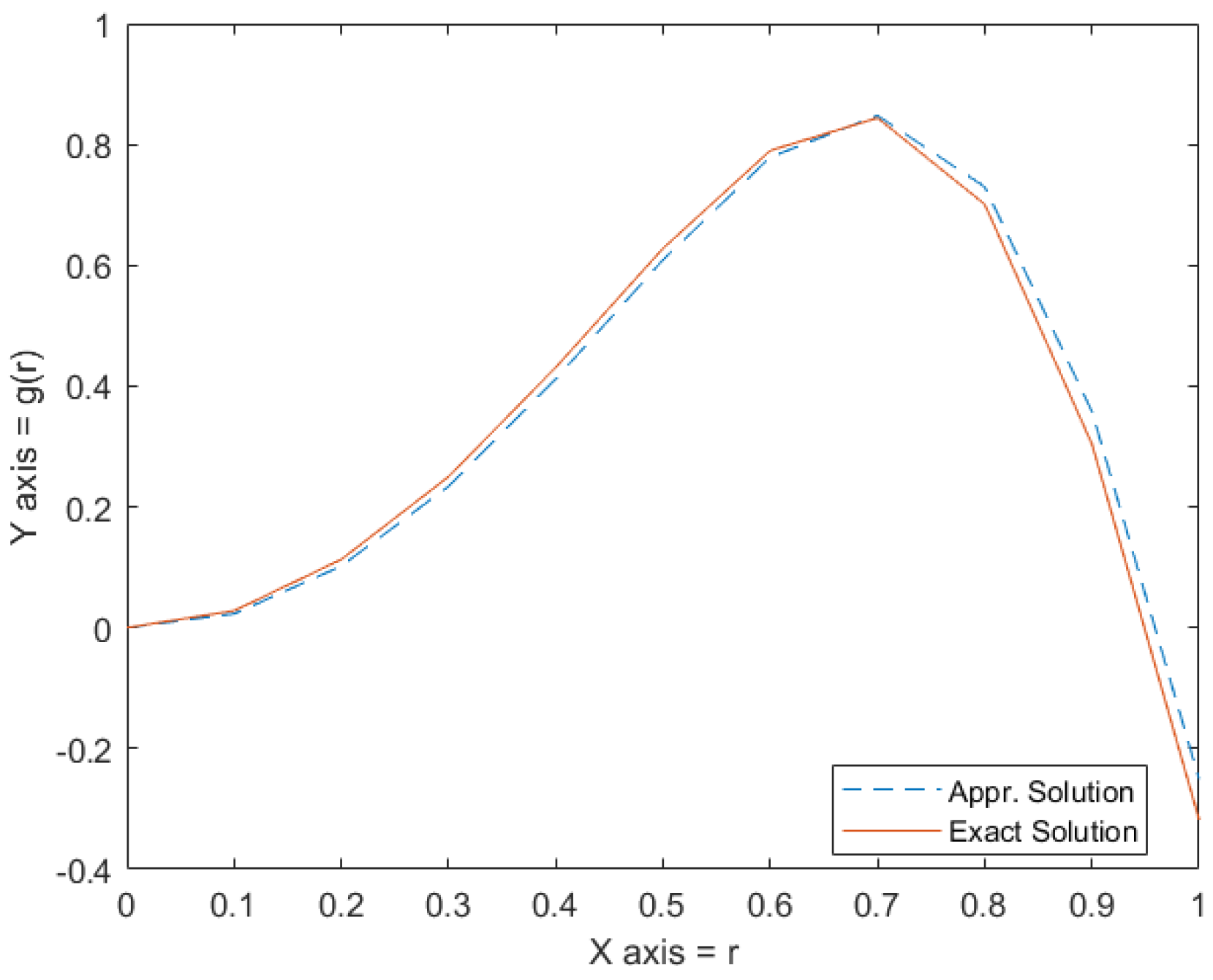
• We are comparing numerical difference between an approximation solution and an exact solution.

Theorem 5.

Let $(\mathcal{V},\perp ,{\mathfrak{w}}_{\mathfrak{b}})$ be an O-complete $B_{b}MS$ with an O-element ${\mathfrak{s}}_0$ and parameter $\delta \ge 1$. Let the two given functions $\alpha :\mathcal{V}\times \mathcal{V}\to {\mathbb{R}}^{+}$ and $\gamma \in {\mathcal{F}}_{\delta }$. Let $\mathfrak{P}:\mathcal{V}\to \mathcal{V}$ be an α-admissible mapping satisfying:

(i) 

$\mathfrak{P}$ is ⊥-preserving.

(ii) 

$\mathfrak{P}$ is $O-G-\alpha$-admissible contraction.

(iii) 

$\mathfrak{P}$ is O-continuous.

• Then, $\mathfrak{P}$ has a UFP.

Proof. 

Consider $(\mathcal{V},\perp )$ is an orthogonal set, there exists

$$\begin{array}{c}\hfill {\mathfrak{s}}_0\in \mathcal{V}:\forall \mathfrak{s}\in \mathcal{V},\mathfrak{s}\perp {\mathfrak{s}}_0\left(or\right)\forall \mathfrak{s}\in \mathcal{V},{\mathfrak{s}}_0\perp \mathfrak{s}.\end{array}$$

It follows that ${\mathfrak{s}}_0\perp \mathfrak{P}{\mathfrak{s}}_0$ or $\mathfrak{P}{\mathfrak{s}}_0\perp {\mathfrak{s}}_0$. Let

$$\begin{array}{c}\hfill {\mathfrak{s}}_1=\mathfrak{P}{\mathfrak{s}}_0,{\mathfrak{s}}_2=\mathfrak{P}{\mathfrak{s}}_1={\mathfrak{P}}^2{\mathfrak{s}}_0\cdots {\mathfrak{s}}_{\widehat{ı}}=\mathfrak{P}{\mathfrak{s}}_{\widehat{ı}-1}={\mathfrak{P}}^{\widehat{ı}}{\mathfrak{s}}_0\forall \widehat{ı}\in \mathbb{N}.\end{array}$$

For any ${\mathfrak{s}}_0\in \mathcal{V}$, set ${\mathfrak{s}}_{\widehat{ı}}=\mathfrak{P}{\mathfrak{s}}_{\widehat{ı}-1}$. Now, we assume that the below cases:

(a)

If $\exists \widehat{ı}\in \mathbb{N}\cup \left\{0\right\}$ such that ${\mathfrak{s}}_{\widehat{ı}}={\mathfrak{s}}_{\widehat{ı}+1}$ then $\mathfrak{P}{\mathfrak{s}}_{\widehat{ı}}={\mathfrak{s}}_{\widehat{ı}}$. It is clear that ${\mathfrak{s}}_{\widehat{ı}}$ is a fixed point of $\mathfrak{P}$. Hence, the proof is complete.

(b)

If ${\mathfrak{s}}_{\widehat{ı}}\ne {\mathfrak{s}}_{\widehat{ı}+1}$, for any $\widehat{ı}\in \mathbb{N}\cup \left\{0\right\}$, then we have ${\mathfrak{w}}_{\mathfrak{b}}({\mathfrak{s}}_{\widehat{ı}+1},{\mathfrak{s}}_{\widehat{ı}})>0$, for each $\widehat{ı}\in \mathbb{N}$.

Since $\mathfrak{P}$ is ⊥-preserving, we have

$$\begin{array}{c}\hfill {\mathfrak{s}}_{\widehat{ı}}\perp {\mathfrak{s}}_{\widehat{ı}+1}\left(\mathrm{or}\right){\mathfrak{s}}_{\widehat{ı}+1}\perp {\mathfrak{s}}_{\widehat{ı}}.\end{array}$$

This implies that $\left\{{\mathfrak{s}}_{\widehat{ı}}\right\}$ is an O-sequence. Since $\mathfrak{P}$ is $\alpha$-admissible, from $\alpha ({\mathfrak{s}}_0,\mathfrak{P}{\mathfrak{s}}_0)\ge 1$ we have

$$\begin{array}{c}\hfill \alpha ({\mathfrak{s}}_0,{\mathfrak{s}}_1)=\alpha ({\mathfrak{s}}_0,\mathfrak{P}{\mathfrak{s}}_0)\ge 1\Rightarrow \alpha (\mathfrak{P}{\mathfrak{s}}_0,\mathfrak{P}{\mathfrak{s}}_1)=\alpha ({\mathfrak{s}}_1,{\mathfrak{s}}_2)\ge 1,\end{array}$$

and inductively,

$$\begin{array}{c}\hfill \alpha ({\mathfrak{s}}_{\widehat{ı}},{\mathfrak{s}}_{\widehat{ı}+1})\ge 1,\forall \widehat{ı}\in \mathbb{N}.\end{array}$$

(3)

Also, from the condition $\alpha ({\mathfrak{s}}_0,T^2{\mathfrak{s}}_0)\ge 1$ we have,

$$\begin{array}{c}\hfill \alpha ({\mathfrak{s}}_0,{\mathfrak{s}}_2)=\alpha ({\mathfrak{s}}_0,{\mathfrak{P}}^2{\mathfrak{s}}_0)\ge 1\Rightarrow \alpha (\mathfrak{P}{\mathfrak{s}}_0,\mathfrak{P}{\mathfrak{s}}_2)=\alpha ({\mathfrak{s}}_1,{\mathfrak{s}}_3)\ge 1,\end{array}$$

(4)

and hence,

$$\begin{array}{c}\hfill \alpha ({\mathfrak{s}}_{\widehat{ı}},{\mathfrak{s}}_{\widehat{ı}+2})\ge 1,\forall \widehat{ı}\in \mathbb{N}.\end{array}$$

Define the O-sequences $\left\{{\mathfrak{q}}_{\widehat{ı}}\right\}$ and $\left\{{\kappa }_{\widehat{ı}}\right\}$ as

$$\begin{array}{c}\hfill {\mathfrak{q}}_{\widehat{ı}}={\mathfrak{w}}_{\mathfrak{b}}({\mathfrak{s}}_{\widehat{ı}-1},{\mathfrak{s}}_{\widehat{ı}}),{\kappa }_{\widehat{ı}}={\mathfrak{w}}_{\mathfrak{b}}({\mathfrak{s}}_{\widehat{ı}-1},{\mathfrak{s}}_{\widehat{ı}+1}).\end{array}$$

We will prove that both the O-sequence $\left\{{\mathfrak{q}}_{\widehat{ı}}\right\}$ and $\left\{{\kappa }_{\widehat{ı}}\right\}$ converge to 0, that is,

$$\begin{array}{c}\hfill \underset{\widehat{ı}\to \infty }{lim}{\mathfrak{w}}_{\mathfrak{b}}({\mathfrak{s}}_{\widehat{ı}-1},{\mathfrak{s}}_{\widehat{ı}})=\underset{\widehat{ı}\to \infty }{lim}{\mathfrak{w}}_{\mathfrak{b}}({\mathfrak{s}}_{\widehat{ı}-1},{\mathfrak{s}}_{\widehat{ı}+1})=0.\end{array}$$

Regarding (3) and the fact that $0\le \gamma \left(\varrho \right)<\frac{1}{\delta }$, the contractive condition (2) with $\mathfrak{s}={\mathfrak{s}}_{\widehat{ı}}$ and $\upsilon ={\mathfrak{s}}_{\widehat{ı}+1}$ becomes

$$\begin{array}{cc}\hfill {\mathfrak{w}}_{\mathfrak{b}}({\mathfrak{s}}_{\widehat{ı}},{\mathfrak{s}}_{\widehat{ı}+1})& ={\mathfrak{w}}_{\mathfrak{b}}(\mathfrak{P}({\mathfrak{s}}_{\widehat{ı}-1},{\mathfrak{s}}_{\widehat{ı}}),\mathfrak{P}({\mathfrak{s}}_{{\widehat{ı}}_1},{\mathfrak{s}}_{\widehat{ı}})\hfill \\ \hfill & \le \alpha ({\mathfrak{s}}_{\widehat{ı}-1},{\mathfrak{s}}_{\widehat{ı}}){\mathfrak{w}}_{\mathfrak{b}}(\mathfrak{P}({\mathfrak{s}}_{\widehat{ı}-1},{\mathfrak{s}}_{\widehat{ı}})\hfill \\ \hfill & \le \gamma \left(\omega ({\mathfrak{s}}_{\widehat{ı}-1},{\mathfrak{s}}_{\widehat{ı}})\right)\mathcal{K}({\mathfrak{s}}_{\widehat{ı}-1},{\mathfrak{s}}_{\widehat{ı}})\hfill \\ \hfill & \le \frac{1}{\delta }\mathcal{K}({\mathfrak{s}}_{\widehat{ı}-1},{\mathfrak{s}}_{\widehat{ı}})\forall \widehat{ı}\ge 1,\hfill \end{array}$$

(5)

where

$$\begin{array}{cc}\hfill \mathcal{K}({\mathfrak{s}}_{\widehat{ı}-1},{\mathfrak{s}}_{\widehat{ı}})& =max\{{\mathfrak{w}}_{\mathfrak{b}}({\mathfrak{s}}_{\widehat{ı}-1},{\mathfrak{s}}_{\widehat{ı}}),{\mathfrak{w}}_{\mathfrak{b}}({\mathfrak{s}}_{\widehat{ı}-1},\mathfrak{P}{\mathfrak{s}}_{\widehat{ı}-1}),{\mathfrak{w}}_{\mathfrak{b}}({\mathfrak{s}}_{\widehat{ı}},\mathfrak{P}{\mathfrak{s}}_{\widehat{ı}})\}\hfill \\ & =max\{{\mathfrak{w}}_{\mathfrak{b}}({\mathfrak{s}}_{\widehat{ı}-1},{\mathfrak{s}}_{\widehat{ı}}),{\mathfrak{w}}_{\mathfrak{b}}({\mathfrak{s}}_{\widehat{ı}-1},{\mathfrak{s}}_{\widehat{ı}}),{\mathfrak{w}}_{\mathfrak{b}}({\mathfrak{s}}_{\widehat{ı}},{\mathfrak{s}}_{\widehat{ı}+1})\}\hfill \\ & =max\{{\mathfrak{w}}_{\mathfrak{b}}({\mathfrak{s}}_{\widehat{ı}-1},{\mathfrak{s}}_{\widehat{ı}}),{\mathfrak{w}}_{\mathfrak{b}}({\mathfrak{s}}_{\widehat{ı}},{\mathfrak{s}}_{\widehat{ı}+1})\}.\hfill \end{array}$$

Suppose that $\mathcal{K}({\mathfrak{s}}_{\widehat{ı}-1},{\mathfrak{s}}_{\widehat{ı}})={\mathfrak{w}}_{\mathfrak{b}}({\mathfrak{s}}_{\widehat{ı}},{\mathfrak{s}}_{\widehat{ı}+1})$ for some $\widehat{ı}\ge 1$. Then, we have

$$\begin{array}{cc}\hfill {\mathfrak{w}}_{\mathfrak{b}}({\mathfrak{s}}_{\widehat{ı}},{\mathfrak{s}}_{\widehat{ı}+1})& \le \gamma \left({\mathfrak{w}}_{\mathfrak{b}}({\mathfrak{s}}_{\widehat{ı}},{\mathfrak{s}}_{\widehat{ı}+1}){\mathfrak{w}}_{\mathfrak{b}}({\mathfrak{s}}_{\widehat{ı}},{\mathfrak{s}}_{\widehat{ı}+1})\right)\hfill \\ & <\frac{1}{\delta }{\mathfrak{w}}_{\mathfrak{b}}({\mathfrak{s}}_{\widehat{ı}},{\mathfrak{s}}_{\widehat{ı}+1})\forall \widehat{ı}\in \mathbb{N},\hfill \end{array}$$

which is a contradiction. Therefore, $\forall \widehat{ı}\ge 1$, $\mathcal{K}({\mathfrak{s}}_{\widehat{ı}-1},{\mathfrak{s}}_{\widehat{ı}})={\mathfrak{w}}_{\mathfrak{b}}({\mathfrak{s}}_{\widehat{ı}-1},{\mathfrak{s}}_{\widehat{ı}})$. In this case, the inequality (5) implies

$$\begin{array}{cc}\hfill {\mathfrak{w}}_{\mathfrak{b}}({\mathfrak{s}}_{\widehat{ı}-1},{\mathfrak{s}}_{\widehat{ı}})& \le \gamma \left({\mathfrak{w}}_{\mathfrak{b}}({\mathfrak{s}}_{\widehat{ı}-1},{\mathfrak{s}}_{\widehat{ı}}){\mathfrak{w}}_{\mathfrak{b}}({\mathfrak{s}}_{\widehat{ı}-1},{\mathfrak{s}}_{\widehat{ı}})\right)\hfill \\ \hfill & <\frac{1}{\delta }{\mathfrak{w}}_{\mathfrak{b}}({\mathfrak{s}}_{\widehat{ı}-1},{\mathfrak{s}}_{\widehat{ı}})\hfill \\ \hfill & <{\mathfrak{w}}_{\mathfrak{b}}({\mathfrak{s}}_{\widehat{ı}-1},{\mathfrak{s}}_{\widehat{ı}})\forall \widehat{ı}\ge 1.\hfill \end{array}$$

(6)

In other words, the positive and decreasing O-sequence $\left\{{\mathfrak{q}}_{\widehat{ı}}\right\}=\left\{{\mathfrak{w}}_{\mathfrak{b}}({\mathfrak{s}}_{\widehat{ı}-1},{\mathfrak{s}}_{\widehat{ı}})\right\}$ is O-convergent to some ${\mathfrak{w}}_{\mathfrak{b}}\ge 0$. Taking limit in (6) we get,

$$\begin{array}{c}\hfill {\mathfrak{w}}_{\mathfrak{b}}=\underset{\widehat{ı}\to \infty }{lim}{\mathfrak{q}}_{\widehat{ı}+1}\le \underset{\widehat{ı}\to \infty }{lim}\gamma \left({\mathfrak{q}}_{\widehat{ı}}\right){\mathfrak{q}}_{\widehat{ı}}={\mathfrak{w}}_{\mathfrak{b}}\underset{\widehat{ı}\to \infty }{lim}\gamma \left({\mathfrak{q}}_{\widehat{ı}}\right)\le \frac{1}{\delta }{\mathfrak{w}}_{\mathfrak{b}}.\end{array}$$

This implies ${lim}_{\widehat{ı}\to \infty }\gamma \left({\mathfrak{q}}_{\widehat{ı}}\right)=\frac{1}{\delta }$ and hence, by (1),

$$\begin{array}{c}\hfill \underset{\widehat{ı}\to \infty }{lim}{\mathfrak{q}}_{\widehat{ı}}=\underset{\widehat{ı}\to \infty }{lim}{\mathfrak{w}}_{\mathfrak{b}}({\mathfrak{s}}_{\widehat{ı}-1},{\mathfrak{s}}_{\widehat{ı}})=0.\end{array}$$

(7)

On the other hand, we observe that repeated application of (6) leads to

$$\begin{array}{c}\hfill {\mathfrak{q}}_{\widehat{ı}+1}<\frac{1}{\delta }{\mathfrak{q}}_{\widehat{ı}}<\frac{1}{{\delta }^2}{\mathfrak{q}}_{\widehat{ı}-1}<\cdots <\frac{1}{{\delta }^{\widehat{ı}+1}}{\mathfrak{q}}_0.\end{array}$$

(8)

Now, taking into account (4), we substitute $\mathfrak{s}={\mathfrak{s}}_{\widehat{ı}-1}$ and $\mathfrak{s}={\mathfrak{s}}_{\widehat{ı}+1}$ in (2). This yields

$$\begin{array}{cc}\hfill {\mathfrak{w}}_{\mathfrak{b}}({\mathfrak{s}}_{\widehat{ı}},{\mathfrak{s}}_{\widehat{ı}+2})& ={\mathfrak{w}}_{\mathfrak{b}}(\mathfrak{P}({\mathfrak{s}}_{\widehat{ı}-1},{\mathfrak{s}}_{\widehat{ı}+1}),\mathfrak{P}({\mathfrak{s}}_{\widehat{ı}-1},{\mathfrak{s}}_{\widehat{ı}+1})\hfill \\ \hfill & \le \alpha ({\mathfrak{s}}_{\widehat{ı}-1},{\mathfrak{s}}_{\widehat{ı}+1}){\mathfrak{w}}_{\mathfrak{b}}(\mathfrak{P}({\mathfrak{s}}_{\widehat{ı}-1},{\mathfrak{s}}_{\widehat{ı}+1})\hfill \\ \hfill & \le \gamma \left(\omega ({\mathfrak{s}}_{\widehat{ı}-1},{\mathfrak{s}}_{\widehat{ı}+1})\right)\mathcal{K}({\mathfrak{s}}_{\widehat{ı}-1},{\mathfrak{s}}_{\widehat{ı}+1})\hfill \\ \hfill & \le \frac{1}{\delta }\mathcal{K}({\mathfrak{s}}_{\widehat{ı}-1},{\mathfrak{s}}_{\widehat{ı}+1})\forall \widehat{ı}\in \mathbb{N},\hfill \end{array}$$

(9)

where

$$\begin{array}{cc}\hfill \mathcal{K}({\mathfrak{s}}_{\widehat{ı}-1},{\mathfrak{s}}_{\widehat{ı}+1})& =max\{{\mathfrak{w}}_{\mathfrak{b}}({\mathfrak{s}}_{\widehat{ı}-1},{\mathfrak{s}}_{\widehat{ı}+1}),{\mathfrak{w}}_{\mathfrak{b}}({\mathfrak{s}}_{\widehat{ı}-1},\mathfrak{P}{\mathfrak{s}}_{\widehat{ı}-1}),{\mathfrak{w}}_{\mathfrak{b}}({\mathfrak{s}}_{\widehat{ı}+1},\mathfrak{P}{\mathfrak{s}}_{\widehat{ı}+1})\},\hfill \\ & =max\{{\mathfrak{w}}_{\mathfrak{b}}({\mathfrak{s}}_{\widehat{ı}-1},{\mathfrak{s}}_{\widehat{ı}+1}),{\mathfrak{w}}_{\mathfrak{b}}({\mathfrak{s}}_{\widehat{ı}-1},{\mathfrak{s}}_{\widehat{ı}}),{\mathfrak{w}}_{\mathfrak{b}}({\mathfrak{s}}_{\widehat{ı}+1},{\mathfrak{s}}_{\widehat{ı}+2})\}.\hfill \end{array}$$

Regarding (6), the maximum $\mathcal{K}({\mathfrak{s}}_{\widehat{ı}-1},{\mathfrak{s}}_{\widehat{ı}+1})$ is either ${\mathfrak{w}}_{\mathfrak{b}}({\mathfrak{s}}_{\widehat{ı}-1},{\mathfrak{s}}_{\widehat{ı}+1})$ or ${\mathfrak{w}}_{\mathfrak{b}}({\mathfrak{s}}_{\widehat{ı}-1},{\mathfrak{s}}_{\widehat{ı}})$, that is, either ${\kappa }_{\widehat{ı}}$ or ${\mathfrak{q}}_{\widehat{ı}}$. From the inequality (9) we have,

$$\begin{array}{c}\hfill {\kappa }_{\widehat{ı}+1}={\mathfrak{w}}_{\mathfrak{b}}({\mathfrak{s}}_{\widehat{ı}},{\mathfrak{s}}_{\widehat{ı}+2})<\frac{1}{\delta }\omega \left({\kappa }_{\widehat{ı}}\right)=\frac{1}{\delta }max\{{\kappa }_{\widehat{ı}},{\mathfrak{q}}_{\widehat{ı}}\}\forall \widehat{ı}\in \mathbb{N}.\end{array}$$

(10)

In addition, from (6) we have,

$$\begin{array}{c}\hfill {\mathfrak{q}}_{\widehat{ı}+1}<{\mathfrak{q}}_{\widehat{ı}}\le max\{{\kappa }_{\widehat{ı}},{\mathfrak{q}}_{\widehat{ı}}\}.\end{array}$$

We deduce that,

$$\begin{array}{c}\hfill max\{{\kappa }_{\widehat{ı}+1},{\mathfrak{q}}_{\widehat{ı}+1}\}\le max\{{\kappa }_{\widehat{ı}},{\mathfrak{q}}_{\widehat{ı}}\}\forall \widehat{ı}\ge 1.\end{array}$$

that is, the O-sequence $max\{{\kappa }_{\widehat{ı}},{\mathfrak{q}}_{\widehat{ı}}\}$ is non increasing and hence, it O-converges to some $\mathfrak{j}\ge 0$. Choose that $\mathfrak{j}>0$. Taking limits we get

$$\begin{array}{cc}\hfill \mathfrak{j}& =\underset{\widehat{ı}\to \infty }{lim}max\{{\kappa }_{\widehat{ı}},{\mathfrak{q}}_{\widehat{ı}}\}\hfill \\ \hfill & =\underset{\widehat{ı}\to \infty }{lim}{\kappa }_{\widehat{ı}}.\hfill \end{array}$$

Alternatively, letting $\widehat{ı}\to \infty$ in (10) we get

$$\begin{array}{c}\hfill \mathfrak{j}=\underset{\widehat{ı}\to \infty }{lim}{\kappa }_{\widehat{ı}+1}<\underset{\widehat{ı}\to \infty }{lim}max\{{\kappa }_{\widehat{ı}},{\mathfrak{q}}_{\widehat{ı}}\}=\mathfrak{j},\end{array}$$

which is a contradiction. Hence $\mathfrak{j}=0$, and then we have,

$$\begin{array}{c}\hfill \underset{\widehat{ı}\to \infty }{lim}{\kappa }_{\widehat{ı}}=\underset{\widehat{ı}\to \infty }{lim}{\mathfrak{w}}_{\mathfrak{b}}({\mathfrak{s}}_{\widehat{ı}-1},{\mathfrak{s}}_{\widehat{ı}+1})=0.\end{array}$$

(11)

Next, we will prove that ${\mathfrak{s}}_{\widehat{ı}}\ne {\mathfrak{s}}_{\widehat{j}}$ for all $\widehat{ı}\ne \widehat{j}$. Assume that ${\mathfrak{s}}_{\widehat{ı}}={\mathfrak{s}}_{\widehat{j}}$ for every $\widehat{ı},\widehat{j}\in \mathbb{N}$ with $\widehat{ı}\ne \widehat{j}$, we have ${\mathfrak{w}}_{\mathfrak{b}}({\mathfrak{s}}_{\widehat{ı}},{\mathfrak{s}}_{\widehat{ı}+1})>0$ for each $\widehat{ı}\in \mathbb{N}$. Without loss of generality, we may take $\widehat{j}>\widehat{ı}+1$. The assumption ${\mathfrak{s}}_{\widehat{ı}}={\mathfrak{s}}_{\widehat{j}}$ implies

$$\begin{array}{c}\hfill {\mathfrak{w}}_{\mathfrak{b}}({\mathfrak{s}}_{\widehat{ı}},\mathfrak{P}{\mathfrak{s}}_{\widehat{ı}})={\mathfrak{w}}_{\mathfrak{b}}({\mathfrak{s}}_{\widehat{j}},\mathfrak{P}{\mathfrak{s}}_{\widehat{j}}).\end{array}$$

Using the inequality (5) we have,

$$\begin{array}{cc}\hfill {\mathfrak{w}}_{\mathfrak{b}}({\mathfrak{s}}_{\widehat{ı}},{\mathfrak{s}}_{\widehat{ı}+1})=& {\mathfrak{w}}_{\mathfrak{b}}({\mathfrak{s}}_{\widehat{ı}},\mathfrak{P}{\mathfrak{s}}_{\widehat{ı}})={\mathfrak{w}}_{\mathfrak{b}}({\mathfrak{s}}_{\widehat{j}},\mathfrak{P}{\mathfrak{s}}_{\widehat{j}})\hfill \\ \hfill =& {\mathfrak{w}}_{\mathfrak{b}}(\mathfrak{P}{\mathfrak{s}}_{\widehat{j}-1},\mathfrak{P}{\mathfrak{s}}_{\widehat{j}})\le \alpha ({\mathfrak{s}}_{\widehat{j}-1}{\mathfrak{s}}_{\widehat{j}}){\mathfrak{w}}_{\mathfrak{b}}({\mathfrak{s}}_{\widehat{j}-1},\mathfrak{P}{\mathfrak{s}}_{\widehat{j}})\hfill \\ \hfill \le & \gamma (\mathcal{K}({\mathfrak{s}}_{\widehat{ı}-1},{\mathfrak{s}}_{\widehat{ı}}))\mathcal{K}({\mathfrak{s}}_{\widehat{j}-1},{\mathfrak{s}}_{\widehat{j}})\hfill \\ \hfill <& \frac{1}{\delta }{\mathfrak{w}}_{\mathfrak{b}}({\mathfrak{s}}_{\widehat{j}-1},{\mathfrak{s}}_{\widehat{j}}),\hfill \end{array}$$

where

$$\begin{array}{cc}\hfill \mathcal{K}({\mathfrak{s}}_{\widehat{j}-1},{\mathfrak{s}}_{\widehat{j}})& =max\{{\mathfrak{w}}_{\mathfrak{b}}({\mathfrak{s}}_{\widehat{j}-1},{\mathfrak{s}}_{\widehat{j}}),{\mathfrak{w}}_{\mathfrak{b}}({\mathfrak{s}}_{\widehat{j}-1},\mathfrak{P}{\mathfrak{s}}_{\widehat{j}-1}),{\mathfrak{w}}_{\mathfrak{b}}({\mathfrak{s}}_{\widehat{j}},\mathfrak{P}{\mathfrak{s}}_{\widehat{j}})\}\hfill \\ & =max\{{\mathfrak{w}}_{\mathfrak{b}}({\mathfrak{s}}_{\widehat{j}-1},{\mathfrak{s}}_{\widehat{j}}),{\mathfrak{w}}_{\mathfrak{b}}({\mathfrak{s}}_{\widehat{j}-1},{\mathfrak{s}}_{\widehat{j}}),{\mathfrak{w}}_{\mathfrak{b}}({\mathfrak{s}}_{\widehat{j}},{\mathfrak{s}}_{\widehat{j}+1})\}\hfill \\ & =max\{{\mathfrak{w}}_{\mathfrak{b}}({\mathfrak{s}}_{\widehat{j}-1},{\mathfrak{s}}_{\widehat{j}}),{\mathfrak{w}}_{\mathfrak{b}}({\mathfrak{s}}_{\widehat{j}},{\mathfrak{s}}_{\widehat{j}+1})\}={\mathfrak{w}}_{\mathfrak{b}}({\mathfrak{s}}_{\widehat{j}-1},{\mathfrak{s}}_{\widehat{j}}).\hfill \end{array}$$

Then, we have

$$\begin{array}{cc}\hfill {\mathfrak{w}}_{\mathfrak{b}}({\mathfrak{s}}_{\widehat{j}},{\mathfrak{s}}_{\widehat{j}+1})& \le \gamma ({\mathfrak{w}}_{\mathfrak{b}}({\mathfrak{s}}_{\widehat{j}-1},{\mathfrak{s}}_{\widehat{j}}){\mathfrak{w}}_{\mathfrak{b}}({\mathfrak{s}}_{\widehat{j}-1},{\mathfrak{s}}_{\widehat{j}}))\hfill \\ & <\frac{1}{\delta }{\mathfrak{w}}_{\mathfrak{b}}({\mathfrak{s}}_{\widehat{j}-1},{\mathfrak{s}}_{\widehat{j}})\hfill \\ & <{\mathfrak{w}}_{\mathfrak{b}}({\mathfrak{s}}_{\widehat{j}-1},{\mathfrak{s}}_{\widehat{j}})\forall \widehat{j}>\widehat{ı}+1.\hfill \end{array}$$

Continuing the process we conclude,

$$\begin{array}{c}\hfill {\mathfrak{w}}_{\mathfrak{b}}({\mathfrak{s}}_{\widehat{j}},{\mathfrak{s}}_{\widehat{j}+1})<{\mathfrak{w}}_{\mathfrak{b}}({\mathfrak{s}}_{\widehat{j}-1},{\mathfrak{s}}_{\widehat{j}})<{\mathfrak{w}}_{\mathfrak{b}}({\mathfrak{s}}_{\widehat{j}-1},{\mathfrak{s}}_{\widehat{j}})<\cdots <{\mathfrak{w}}_{\mathfrak{b}}({\mathfrak{s}}_{\widehat{ı}},{\mathfrak{s}}_{\widehat{ı}+1}),\end{array}$$

which contradicts the assumption ${\mathfrak{s}}_{\widehat{ı}}={\mathfrak{s}}_{\widehat{j}}$ for some $\widehat{ı}\ne \widehat{j}$. Hence ${\mathfrak{s}}_{\widehat{ı}}\ne {\mathfrak{s}}_{\widehat{j}}$ for all $\widehat{ı}\ne \widehat{j}$.

Now to prove that $\left\{{\mathfrak{s}}_{\widehat{ı}}\right\}$ is a O-Cauchy sequence, that is,

$$\begin{array}{c}\hfill \underset{\widehat{ı}\to \infty }{lim}{\mathfrak{w}}_{\mathfrak{b}}({\mathfrak{s}}_{\widehat{ı}},{\mathfrak{s}}_{\widehat{ı}+\zeta })=0,\forall \zeta \in \mathbb{N}.\end{array}$$

(12)

Notice that (12) is satisfied for $\zeta =1$ and $\zeta =2$ due to (7) and (11). Hence, we choose $\zeta \le 3$. Now we consider two cases, for $\zeta \in \mathbb{N}$.

Case 1. Consider $\zeta =2\widehat{j}+1$ where $\widehat{j}\ge 1$. We have ${\mathfrak{s}}_{\mathfrak{j}}\ne {\mathfrak{s}}_{\delta }$ for all $\mathfrak{j}\ne \delta$ and ${\mathfrak{s}}_{\mathfrak{j}}\ne {\mathfrak{s}}_{\mathfrak{j}+1}\mathit{for}\mathit{all}\mathfrak{j}\ge 0$. We use the inequality $\left(B3\right)$ in (3), hence,

$$\begin{array}{cc}\hfill {\mathfrak{w}}_{\mathfrak{b}}({\mathfrak{s}}_{\widehat{ı}},{\zeta }_{\mathfrak{n}+\mathfrak{k}})=& {\mathfrak{w}}_{\mathfrak{b}}({\mathfrak{s}}_{\widehat{ı}},{\mathfrak{s}}_{\widehat{ı}+2\widehat{j}+1})\le \delta [{\mathfrak{w}}_{\mathfrak{b}}({\mathfrak{s}}_{\widehat{ı}},{\mathfrak{s}}_{\widehat{ı}+1})+{\mathfrak{w}}_{\mathfrak{b}}({\mathfrak{s}}_{\widehat{ı}+1},{\mathfrak{s}}_{\widehat{ı}+2})+{\mathfrak{w}}_{\mathfrak{b}}({\mathfrak{s}}_{\widehat{ı}+2},{\mathfrak{s}}_{\widehat{ı}+2\widehat{j}+1})]\hfill \\ \hfill \le & \delta [{\mathfrak{w}}_{\mathfrak{b}}({\mathfrak{s}}_{\widehat{ı}},{\mathfrak{s}}_{\widehat{ı}+1})+{\mathfrak{w}}_{\mathfrak{b}}({\mathfrak{s}}_{\widehat{ı}+1},{\mathfrak{s}}_{\widehat{ı}+2})]\hfill \\ & +{\delta }^2[{\mathfrak{w}}_{\mathfrak{b}}({\mathfrak{s}}_{\widehat{ı}+2},{\mathfrak{s}}_{\widehat{ı}+3})+{\mathfrak{w}}_{\mathfrak{b}}({\mathfrak{s}}_{\widehat{ı}+3},{\mathfrak{s}}_{\widehat{ı}+4})+{\mathfrak{w}}_{\mathfrak{b}}({\mathfrak{s}}_{\widehat{ı}+4},{\mathfrak{s}}_{\widehat{ı}+2\widehat{j}+1})]\hfill \\ \hfill ⋮\\ \hfill \le & \delta [{\mathfrak{w}}_{\mathfrak{b}}({\mathfrak{s}}_{\widehat{ı}},{\mathfrak{s}}_{\widehat{ı}+1})+{\mathfrak{w}}_{\mathfrak{b}}({\mathfrak{s}}_{\widehat{ı}+1},{\mathfrak{s}}_{\widehat{ı}+2})]+{\delta }^2[{\mathfrak{w}}_{\mathfrak{b}}({\mathfrak{s}}_{\widehat{ı}+2},{\mathfrak{s}}_{\widehat{ı}+3})+{\mathfrak{w}}_{\mathfrak{b}}({\mathfrak{s}}_{\widehat{ı}+3},{\mathfrak{s}}_{\widehat{ı}+4})]\hfill \\ \hfill & +{\delta }^3[{\mathfrak{w}}_{\mathfrak{b}}({\mathfrak{s}}_{\widehat{ı}+4},{\mathfrak{s}}_{\widehat{ı}+5})+{\mathfrak{w}}_{\mathfrak{b}}({\mathfrak{s}}_{\widehat{ı}+5},{\mathfrak{s}}_{\widehat{ı}+6})]+\dots +{\delta }^{\widehat{j}+1}[{\mathfrak{w}}_{\mathfrak{b}}({\mathfrak{s}}_{\widehat{ı}+2\widehat{j}},{\mathfrak{s}}_{\widehat{ı}+2\widehat{j}+1})]\hfill \\ \hfill \le & \delta [{\mathfrak{w}}_{\mathfrak{b}}({\mathfrak{s}}_{\widehat{ı}},{\mathfrak{s}}_{\widehat{ı}+1})+{\delta }^2[{\mathfrak{w}}_{\mathfrak{b}}({\mathfrak{s}}_{\widehat{ı}+1},{\mathfrak{s}}_{\widehat{ı}+2})+{\delta }^3[{\mathfrak{w}}_{\mathfrak{b}}({\mathfrak{s}}_{\widehat{ı}+2},{\mathfrak{s}}_{\widehat{ı}+3})+\cdots \hfill \\ & +{\delta }^{\widehat{ı}+2\widehat{j}-1}{\mathfrak{w}}_{\mathfrak{b}}({\mathfrak{s}}_{\widehat{ı}+2\widehat{j}},{\mathfrak{s}}_{\widehat{ı}+2\widehat{j}+1}).\hfill \end{array}$$

Then, by the inequality (8) we conclude

$$\begin{array}{cc}\hfill {\mathfrak{w}}_{\mathfrak{b}}({\mathfrak{s}}_{\widehat{ı}},{\mathfrak{s}}_{\widehat{ı}+\zeta })& \le \frac{1}{{\delta }^{\widehat{ı}+1}}{\mathfrak{w}}_{\mathfrak{b}}({\mathfrak{s}}_0,{\mathfrak{s}}_1)+\frac{1}{{\delta }^{\widehat{ı}}}{\mathfrak{w}}_{\mathfrak{b}}({\mathfrak{s}}_0,{\mathfrak{s}}_1)+\cdots +\frac{1}{{\delta }^{\widehat{ı}+2\widehat{j}}}{\mathfrak{w}}_{\mathfrak{b}}({\mathfrak{s}}_0,{\mathfrak{s}}_1)\hfill \\ & ={\mathfrak{w}}_{\mathfrak{b}}({\mathfrak{s}}_0,{\mathfrak{s}}_1)\left[\sum _{\zeta =0}^{\widehat{ı}+2\widehat{j}}\frac{1}{{\delta }^{\widehat{ı}}}-\sum _{\zeta =0}^{\widehat{ı}-2}\frac{1}{{\delta }^{\widehat{ı}}}\right]\hfill \\ \hfill & ={\mathfrak{w}}_{\mathfrak{b}}({\mathfrak{s}}_0,{\mathfrak{s}}_1)\left[\frac{{\delta }^{\widehat{ı}+2\widehat{j}+1}-1}{{\delta }^{\widehat{ı}+2\widehat{j}(\delta -1)}}-\frac{{\delta }^{\widehat{ı}-1}-1}{{\delta }^{\widehat{ı}-2(\delta -1)}}\right].\hfill \end{array}$$

Letting $\widehat{ı}\to \infty$ in the above inequality, we get

$$\begin{array}{c}\hfill 0\le \underset{\widehat{ı}\to \infty }{lim}{\mathfrak{w}}_{\mathfrak{b}}({\mathfrak{s}}_{\widehat{ı}},{\mathfrak{s}}_{\widehat{ı}+\zeta })\le \underset{\widehat{ı}\to \infty }{lim}{\mathfrak{w}}_{\mathfrak{b}}({\mathfrak{s}}_0,{\mathfrak{s}}_1)\left[\frac{{\delta }^{\widehat{ı}+2\widehat{j}+1}-1}{{\delta }^{\widehat{ı}+2\widehat{j}(\delta -1)}}-\frac{{\delta }^{\widehat{ı}-1}-1}{{\delta }^{\widehat{ı}-2(\delta -1)}}\right]=0.\end{array}$$

Case 2. Consider $\zeta =2\widehat{j}$ where $\widehat{j}\ge 2$. Again, using the inequality (B3) in Definition 3, we obtain

$$\begin{array}{cc}\hfill {\mathfrak{w}}_{\mathfrak{b}}({\mathfrak{s}}_{\widehat{ı}},{\zeta }_{\mathfrak{n}+\mathfrak{k}})=& {\mathfrak{w}}_{\mathfrak{b}}({\mathfrak{s}}_{\widehat{ı}},{\mathfrak{s}}_{\widehat{ı}+2\widehat{j}})\le \delta [{\mathfrak{w}}_{\mathfrak{b}}({\mathfrak{s}}_{\widehat{ı}},{\mathfrak{s}}_{\widehat{ı}+1})+{\mathfrak{w}}_{\mathfrak{b}}({\mathfrak{s}}_{\widehat{ı}+1},{\mathfrak{s}}_{\widehat{ı}+2})+{\mathfrak{w}}_{\mathfrak{b}}({\mathfrak{s}}_{\widehat{ı}+2},{\mathfrak{s}}_{\widehat{ı}+2\widehat{j}})]\hfill \\ \hfill \le & \delta [{\mathfrak{w}}_{\mathfrak{b}}({\mathfrak{s}}_{\widehat{ı}},{\mathfrak{s}}_{\widehat{ı}+1})+{\mathfrak{w}}_{\mathfrak{b}}({\mathfrak{s}}_{\widehat{ı}+1},{\mathfrak{s}}_{\widehat{ı}+2})]\hfill \\ & +{\delta }^2[{\mathfrak{w}}_{\mathfrak{b}}({\mathfrak{s}}_{\widehat{ı}+2},{\mathfrak{s}}_{\widehat{ı}+3})+{\mathfrak{w}}_{\mathfrak{b}}({\mathfrak{s}}_{\widehat{ı}+3},{\mathfrak{s}}_{\widehat{ı}+4})+{\mathfrak{w}}_{\mathfrak{b}}({\mathfrak{s}}_{\widehat{ı}+4},{\mathfrak{s}}_{\widehat{ı}+2\widehat{j}})]\hfill \\ \hfill \le & \delta [{\mathfrak{w}}_{\mathfrak{b}}({\mathfrak{s}}_{\widehat{ı}},{\mathfrak{s}}_{\widehat{ı}+1})+{\mathfrak{w}}_{\mathfrak{b}}({\mathfrak{s}}_{\widehat{ı}+1},{\mathfrak{s}}_{\widehat{ı}+2})]+{\delta }^2[{\mathfrak{w}}_{\mathfrak{b}}({\mathfrak{s}}_{\widehat{ı}+2},{\mathfrak{s}}_{\widehat{ı}+3})+{\mathfrak{w}}_{\mathfrak{b}}({\mathfrak{s}}_{\widehat{ı}+3},{\mathfrak{s}}_{\widehat{ı}+4})]\hfill \\ \hfill & +\cdots +{\delta }^{\widehat{j}-1}[{\mathfrak{w}}_{\mathfrak{b}}({\mathfrak{s}}_{\widehat{ı}+2\widehat{j}-4},{\mathfrak{s}}_{\widehat{ı}+2\widehat{j}-3})+{\mathfrak{w}}_{\mathfrak{b}}({\mathfrak{s}}_{\widehat{ı}+2\widehat{j}-3},{\mathfrak{s}}_{\widehat{ı}+2\widehat{j}-2})\hfill \\ & +{\mathfrak{w}}_{\mathfrak{b}}({\mathfrak{s}}_{\widehat{ı}+2\widehat{j}-2},{\mathfrak{s}}_{\widehat{ı}+2\widehat{j}})]\hfill \\ \hfill \le & \delta [{\mathfrak{w}}_{\mathfrak{b}}({\mathfrak{s}}_{\widehat{ı}},{\mathfrak{s}}_{\widehat{ı}+1})+{\delta }^2[{\mathfrak{w}}_{\mathfrak{b}}({\mathfrak{s}}_{\widehat{ı}+1},{\mathfrak{s}}_{\widehat{ı}+2})+{\delta }^3[{\mathfrak{w}}_{\mathfrak{b}}({\mathfrak{s}}_{\widehat{ı}+2},{\mathfrak{s}}_{\widehat{ı}+3})+\cdots \hfill \\ & +{\delta }^{\widehat{ı}+2\widehat{j}-3}{\mathfrak{w}}_{\mathfrak{b}}({\mathfrak{s}}_{\widehat{ı}+2\widehat{j}-3},{\mathfrak{s}}_{\widehat{ı}+2\widehat{j}-2})+{\delta }^{\widehat{j}-1}{\mathfrak{w}}_{\mathfrak{b}}({\mathfrak{s}}_{\widehat{ı}+2\widehat{j}-2},{\mathfrak{s}}_{\widehat{ı}+2\widehat{j}}).\hfill \end{array}$$

By the inequality in (8), we have

$$\begin{array}{cc}\hfill {\mathfrak{w}}_{\mathfrak{b}}({\mathfrak{s}}_{\widehat{ı}},{\mathfrak{s}}_{\widehat{ı}+\zeta })& \le \frac{1}{{\delta }^{\widehat{ı}+1}}{\mathfrak{w}}_{\mathfrak{b}}({\mathfrak{s}}_0,{\mathfrak{s}}_1)+\frac{1}{{\delta }^{\widehat{ı}}}{\mathfrak{w}}_{\mathfrak{b}}({\mathfrak{s}}_0,{\mathfrak{s}}_1)+\cdots +\frac{1}{{\delta }^{\widehat{ı}+2\widehat{j}-2}}{\mathfrak{w}}_{\mathfrak{b}}({\mathfrak{s}}_0,{\mathfrak{s}}_1)\hfill \\ \hfill & +{\delta }^{\widehat{j}-1}{\mathfrak{w}}_{\mathfrak{b}}({\mathfrak{s}}_{\widehat{ı}+2\widehat{j}-2},{\mathfrak{s}}_{\widehat{ı}+2\widehat{j}})\hfill \\ \hfill & ={\mathfrak{w}}_{\mathfrak{b}}({\mathfrak{s}}_0,{\mathfrak{s}}_1)\left[\sum _{\zeta =0}^{\widehat{ı}+2{\widehat{j}}_2}\frac{1}{{\delta }^{\zeta }}-\sum _{\zeta =0}^{\widehat{ı}-2}\frac{1}{{\delta }^{\zeta }}\right]+{\delta }^{\widehat{j}-1}{\mathfrak{w}}_{\mathfrak{b}}({\mathfrak{s}}_{\widehat{ı}+2\widehat{j}-2},{\mathfrak{s}}_{\widehat{ı}+2\widehat{j}})\hfill \\ \hfill & ={\mathfrak{w}}_{\mathfrak{b}}({\mathfrak{s}}_0,{\mathfrak{s}}_1)\left[\frac{{\delta }^{\widehat{ı}+2\widehat{j}+1}-1}{{\delta }^{\widehat{ı}+2\widehat{j}(\delta -1)}}-\frac{{\delta }^{\widehat{ı}-1}-1}{{\delta }^{\widehat{ı}-2(\delta -1)}}\right]+{\delta }^{\widehat{j}-1}{\mathfrak{w}}_{\mathfrak{b}}({\mathfrak{s}}_{\widehat{ı}+2\widehat{j}-2},{\mathfrak{s}}_{\widehat{ı}+2\widehat{j}}).\hfill \end{array}$$

(13)

From (11) we have ${lim}_{\widehat{ı}\to \infty }{\delta }^{\widehat{j}-1}{\mathfrak{w}}_{\mathfrak{b}}({\mathfrak{s}}_{\widehat{ı}+2\widehat{j}-2},{\mathfrak{s}}_{\widehat{ı}+2\widehat{j}})=0$ and hence, using (13) we obtain

$$\begin{array}{cc}\hfill 0& \le \underset{\widehat{ı}\to \infty }{lim}{\mathfrak{w}}_{\mathfrak{b}}({\mathfrak{s}}_{\widehat{ı}},{\mathfrak{s}}_{\widehat{ı}+\zeta })\hfill \\ & \le \underset{\widehat{ı}\to \infty }{lim}\{{\mathfrak{w}}_{\mathfrak{b}}({\mathfrak{s}}_0,{\mathfrak{s}}_1)\left[\frac{{\delta }^{\widehat{ı}+2\widehat{j}+1}-1}{{\delta }^{\widehat{ı}+2\widehat{j}(\delta -1)}}-\frac{{\delta }^{\widehat{ı}-1}-1}{{\delta }^{\widehat{ı}-2(\delta -1)}}\right]+{\delta }^{\widehat{j}-1}{\mathfrak{w}}_{\mathfrak{b}}({\mathfrak{s}}_{\widehat{ı}+2\widehat{j}-2},{\mathfrak{s}}_{\widehat{ı}+2\widehat{j}})\}=0,\hfill \\ \hfill \underset{\widehat{ı}\to \infty }{lim}{\mathfrak{w}}_{\mathfrak{b}}({\mathfrak{s}}_{\widehat{ı}},{\mathfrak{s}}_{\widehat{ı}+\zeta })& =0.\hfill \end{array}$$

Therefore, O-sequence $\left\{{\mathfrak{s}}_{\widehat{ı}}\right\}$ in $(\mathcal{V},{\mathfrak{w}}_{\mathfrak{b}})$ is O-Cauchy sequence. Since $(\mathcal{V},{\mathfrak{w}}_{\mathfrak{b}})$ is a O-complete $O{B}_{b}MS$, there exists $\omega \in \mathcal{V}$ such that

$$\begin{array}{c}\hfill \underset{\widehat{ı}\to \infty }{lim}{\mathfrak{w}}_{\mathfrak{b}}({\mathfrak{s}}_{\widehat{ı}},\omega )=0.\end{array}$$

(14)

Since $\mathfrak{P}$ is a O-continuous map, from (14) we get

$$\begin{array}{c}\hfill \underset{\widehat{ı}\to \infty }{lim}{\mathfrak{w}}_{\mathfrak{b}}(\mathfrak{P}{\mathfrak{s}}_{\widehat{ı}},\mathfrak{P}\omega )=\underset{\widehat{ı}\to \infty }{lim}{\mathfrak{w}}_{\mathfrak{b}}({\mathfrak{s}}_{\widehat{ı}+1},\mathfrak{P}\omega )=0,\end{array}$$

that is, the O-Cauchy sequence $\left\{{\mathfrak{s}}_{\widehat{ı}}\right\}$ is O-convergent to $\mathfrak{P}\omega$. Then the proposition (1) implies that $\mathfrak{P}\omega =\omega$, i.e., $\omega$ is a fixed point of $\mathfrak{P}$.

Since $\gamma \in {\mathcal{F}}_{\delta }$, we conclude ${lim}_{\widehat{ı}\to \infty }\omega ({\mathfrak{s}}_{\widehat{ı}},\omega )=0$. Therefore, $\omega =\mathfrak{P}\omega$. We prove now the point $\omega \in \mathcal{V}$ is unique.

Assume that $\omega$ and $\mu$ are distinct fixed points of $\mathfrak{P}$. Suppose that, ${\mathfrak{P}}^{\widehat{ı}}\omega =\omega \ne \mu ={\mathfrak{P}}^{\widehat{ı}}\mu$ for all $\widehat{ı}\in \mathbb{N}$. By choice of ${\mathfrak{s}}_0$ in the first part of proof, we obtain

$$\begin{array}{c}\hfill ({\mathfrak{s}}_0\perp \omega ,{\mathfrak{s}}_0\perp \mu )\mathrm{or}(\omega \perp {\mathfrak{s}}_0,\mu \perp {\mathfrak{s}}_0).\end{array}$$

Since $\mathfrak{P}$ is ⊥-preserving, we have

$$\begin{array}{c}\hfill ({\mathfrak{P}}^{\widehat{ı}}{\mathfrak{s}}_0\perp {\mathfrak{P}}^{\widehat{ı}}\omega ,{\mathfrak{P}}^{\widehat{ı}}{\mathfrak{s}}_0\perp {\mathfrak{P}}^{\widehat{ı}}\mu )\mathrm{or}({\mathfrak{P}}^{\widehat{ı}}\omega \perp {\mathfrak{P}}^{\widehat{ı}}{\mathfrak{s}}_0,{\mathfrak{P}}^{\widehat{ı}}\mu \perp {\mathfrak{P}}^{\widehat{ı}}{\mathfrak{s}}_0),\end{array}$$

for all $\widehat{ı}\in \mathbb{N}$. Since $\mathfrak{P}$ is an orthogonal Geragthy contraction, we get

$$\begin{array}{c}\hfill {\mathfrak{w}}_{\mathfrak{b}}(\omega ,\mu )={\mathfrak{w}}_{\mathfrak{b}}(\mathfrak{P}\omega ,\mathfrak{P}\mu )\le \gamma \left(\mathcal{K}(\omega ,\mu )\right)\mathcal{K}(\omega ,\mu ),\end{array}$$

where

$$\begin{array}{cc}\hfill \mathcal{K}(\omega ,\mu )& =max\{{\mathfrak{w}}_{\mathfrak{b}}(\omega ,\mu ),{\mathfrak{w}}_{\mathfrak{b}}(\omega ,\mathfrak{P}\omega ),{\mathfrak{w}}_{\mathfrak{b}}(\mu ,\mathfrak{P}\mu )\}\hfill \\ & \le {\mathfrak{w}}_{\mathfrak{b}}(\omega ,\mu ).\hfill \end{array}$$

Therefore, we have ${\mathfrak{w}}_{\mathfrak{b}}(\omega ,\mu )<\frac{1}{\delta }{\mathfrak{w}}_{\mathfrak{b}}(\omega ,\mu )$, which is a contradiction. Then, $\omega =\mu$. Hence $\mathfrak{P}$ has a UFP in $\mathcal{V}$. □

Corollary 1.

Let $(\mathcal{V},{\mathfrak{w}}_{\mathfrak{b}})$ be an O-complete $B_{b}MS$ with a parameter $\delta \ge 1$ and let $\gamma \in {\mathcal{F}}_{\delta }$ be a function. Let $\mathfrak{P}:\mathcal{V}\to \mathcal{V}$ be an O-continuous self mapping satisfying

$$\begin{array}{cc}\hfill \mathfrak{s}\perp \upsilon \mathit{or}& \upsilon \perp \mathfrak{s},{\mathfrak{w}}_{\mathfrak{b}}(\mathfrak{P}\mathfrak{s},\mathfrak{P}\upsilon )>0\hfill \\ \hfill & \Rightarrow {\mathfrak{w}}_{\mathfrak{b}}(\mathfrak{P}\mathfrak{s},\mathfrak{P}\upsilon )\le \gamma \left({\mathfrak{w}}_{\mathfrak{b}}(\mathfrak{s},\upsilon )\right){\mathfrak{w}}_{\mathfrak{b}}(\mathfrak{s},\upsilon ),\forall \mathfrak{s},\upsilon \in \mathcal{V}.\hfill \end{array}$$

Then, $\mathfrak{P}$ has a UFP.

Next, we give an example to support our Theorem (5).

Example 3.

Let $\mathcal{V}=\mathcal{I}\cup \mathcal{J}$ where $\mathcal{I}=\{\frac{1}{2},\frac{1}{4},\frac{1}{6},\frac{1}{8}\}$ and $\mathcal{J}=[1,2]$. Define the binary relation ⊥ on $\mathcal{V}$ by $\mathfrak{s}\perp \upsilon$ if $\mathfrak{s},\upsilon \ge 0$. Define the function ${\mathfrak{w}}_{\mathfrak{b}}:\mathcal{V}\times \mathcal{V}\to {\mathbb{R}}^{+}$ such that ${\mathfrak{w}}_{\mathfrak{b}}(\mathfrak{s},\upsilon )={\mathfrak{w}}_{\mathfrak{b}}(\upsilon ,\mathfrak{s})$ as follows:

For $\mathfrak{s},\upsilon \in \mathcal{V}$ or $\mathfrak{s}\in \mathcal{I}$ and $\upsilon \in \mathcal{J}$, ${\mathfrak{w}}_{\mathfrak{b}}(\mathfrak{s},\upsilon )=|\mathfrak{s}-\upsilon |$ and

$$\begin{array}{cc}\hfill {\mathfrak{w}}_{\mathfrak{b}}(\frac{1}{2},\frac{1}{4})& ={\mathfrak{w}}_{\mathfrak{b}}(\frac{1}{6},\frac{1}{8})=0.2.\hfill \\ \hfill {\mathfrak{w}}_{\mathfrak{b}}(\frac{1}{2},\frac{1}{6})& ={\mathfrak{w}}_{\mathfrak{b}}(\frac{1}{4},\frac{1}{6})={\mathfrak{w}}_{\mathfrak{b}}(\frac{1}{4},\frac{1}{8})=0.1.\hfill \\ \hfill {\mathfrak{w}}_{\mathfrak{b}}(\frac{1}{2},\frac{1}{8})& =1.\hfill \end{array}$$

Clearly, $(\mathcal{V},\perp ,{\mathfrak{w}}_{\mathfrak{b}})$ is an O-complete $B_{b}MS$ with constant $\delta =\frac{10}{3}$. Let $\mathfrak{P}:\mathcal{V}\to \mathcal{V}$ be defined as

$$\mathfrak{P}\mathfrak{s}=\left\{\begin{array}{cc}\frac{\mathfrak{s}}{8}\hfill & if\mathfrak{s}\in \mathcal{J}\hfill \\ \frac{1}{6}\hfill & if\mathfrak{s}\in \mathcal{I}.\hfill \end{array}\right.$$

Clearly, $\mathfrak{P}$ is an ⊥-preserving. Now, we verify that $\mathfrak{P}$ is an orthogonal Geraghty type α-admissible contraction. We see that

$${\mathfrak{w}}_{\mathfrak{b}}(\mathfrak{P}\mathfrak{s},\mathfrak{P}\upsilon )=\left\{\begin{array}{cc}0\hfill & if\mathfrak{s},\upsilon \in \mathcal{I}\hfill \\ 0.2\hfill & if\mathfrak{s}\in \mathcal{I},\upsilon =1\hfill \\ 0.1\hfill & if\mathfrak{s}\in \mathcal{I},\upsilon =2\hfill \\ 0.1\hfill & if\mathfrak{s},\upsilon \in \mathcal{J}.\hfill \end{array}\right.$$

Then, for all $\mathfrak{s},\upsilon \in \mathcal{V}$ the mapping $\mathfrak{P}$ satisfies the condition

$$\begin{array}{c}\hfill {\mathfrak{w}}_{\mathfrak{b}}(\mathfrak{P}\mathfrak{s},\mathfrak{P}\upsilon )\le \frac{3}{20}{\mathfrak{w}}_{\mathfrak{b}}(\mathfrak{s},\upsilon )=\frac{1\setminus 2}{10\setminus 3}{\mathfrak{w}}_{\mathfrak{b}}(\mathfrak{s},\upsilon ).\end{array}$$

Consider a mapping $\mathfrak{P}:[0,\infty )\to \mathcal{R}$ defined by $\mathfrak{P}\left(\mathfrak{s}\right)=\mathfrak{s}$, it is clearly that $\gamma \in {\mathcal{F}}_{\delta }$, and we get

$$\begin{array}{c}\hfill {\mathfrak{w}}_{\mathfrak{b}}(\mathfrak{P}\mathfrak{s},\mathfrak{P}\upsilon )\le \gamma \left(\mathcal{K}(\mathfrak{s},\upsilon )\right)\mathcal{K}(\mathfrak{s},\upsilon )\forall \mathfrak{s},\upsilon \in \mathcal{V}.\end{array}$$

Hence, the condition of Corollary 1 holds with $\gamma \left(\varrho \right)=\frac{1}{2\delta }=\frac{3}{20}$ and $\mathfrak{P}$ has a UFP which is $\mathfrak{s}=\frac{1}{6}$.

4. Applications

As an application of Theorem 5, we find the existence and uniqueness of the following integral equation:

$$\begin{array}{c}\hfill \omega \left(\varrho \right)=\lambda \left(\varrho \right)+{\int }_0^{\mathfrak{a}}\mathcal{G}(\varrho ,\delta )\mathcal{H}(\varrho ,\delta ,\omega \left(\delta \right))d\delta ,\varrho \in [0,\mathfrak{a}],\mathfrak{a}>0.\end{array}$$

(15)

Consider $\mathcal{V}=\mathcal{C}\left(\right[0,\mathfrak{a}],\mathbb{R})$ be a real continuous functions on $[0,\mathfrak{a}]$ and $\mathfrak{P}:\mathcal{V}\to \mathcal{V}$ the mapping defined by

$$\begin{array}{c}\hfill {\mathfrak{w}}_{\mathfrak{b}}(\omega ,\mu )=\underset{0\le \varrho \le \mathfrak{a}}{max}{|\omega \left(\varrho \right)-\mu \left(\varrho \right)|}^2,\omega ,\mu \in \mathcal{V}.\end{array}$$

(16)

Obviously, $(\mathcal{V},\mathfrak{w})$ is a complete b-metric space with constant $\delta =2$ and $\omega \left(\varrho \right)$ is a solution of the Equation (15) iff $\omega \left(\varrho \right)$ is a fixed point of $\mathfrak{P}$.

Theorem 6.

Suppose that

$\left(R_1\right)$

The mappings $\mathcal{G}:[0,\mathfrak{a}]\times \mathbb{R}\to {\mathbb{R}}^{+}$, $\mathcal{H}:[0,\mathfrak{a}]\times \mathbb{R}\to \mathbb{R},$ and $\lambda :[0,\mathfrak{a}]\to \mathbb{R}$ are O-continuous functions.

$\left(R_2\right)$

There exists, for all $\varrho ,\delta \in [0,\mathfrak{a}]$ and $\omega ,\mu \in \mathcal{V}$ such that

$$\begin{array}{c}\hfill |\mathcal{H}(\varrho ,\delta ,\omega \left(\delta \right))-\mathcal{H}(\varrho ,\delta ,\mu \left(\delta \right))|\le \sqrt{\frac{e^{-\mathcal{K}(\omega ,\mu )}\mathcal{K}(\omega ,\mu )}{2}}.\end{array}$$

(17)

$\left(R_3\right)$

For all $\varrho ,\delta \in [0,\mathfrak{a}]$, we have

$$\begin{array}{c}\hfill max{\int }_0^{\mathfrak{a}}\mathcal{G}{(\varrho ,\delta )}^{2}d\delta \le \frac{1}{\mathfrak{a}}.\end{array}$$

Then, (15) has a unique solution in $\mathcal{V}$.

Proof. 

Consider the O-relation ⊥ on $\mathcal{V}$ defined by

$$\begin{array}{c}\hfill \omega \perp \mu \iff \omega \left(\varrho \right)\mu \left(\varrho \right)\ge \omega \left(\varrho \right)or\omega \left(\varrho \right)\mu \left(\varrho \right)\ge \mu \left(\varrho \right),\forall \varrho \in [0,\mathfrak{a}].\end{array}$$

Then $(\mathcal{V},\perp )$ is an O-set. In fact, if $\left\{{\omega }_{\widehat{ı}}\right\}$ is an arbitrary Cauchy O-sequence in $\mathcal{V}$, then there exists a subsequence $\left\{{\omega }_{\widehat{{ı}_{\mathfrak{n}}}}\right\}$ of $\left\{{\omega }_{\widehat{ı}}\right\}$ for which ${\omega }_{\widehat{{ı}_{\mathfrak{n}}}}=0$ for all $\mathfrak{n}\ge 1$ or there exists a monotone subsequence $\left\{{\omega }_{\widehat{{ı}_{\mathfrak{n}}}}\right\}$ of $\left\{{\omega }_{\widehat{ı}}\right\}$ for which ${\omega }_{\widehat{{ı}_{\mathfrak{n}}}}\le \frac{1}{2}$ for all $\mathfrak{n}\ge 1$. It follows that $\left\{{\omega }_{\widehat{{ı}_{\mathfrak{n}}}}\right\}$ converges to a point $\omega \in [0,\frac{1}{2}]\subset \mathcal{V}$. Therefore, $(\mathcal{V},\perp ,{\mathfrak{w}}_{\mathfrak{b}})$ is an O-complete $B_{b}MS$ with parameter $\delta =2$. For each $\omega ,\mu \in \mathcal{V}$ with $\omega \perp \mu$ and $\varrho \in [0,\mathfrak{a}]$, we have

$$\begin{array}{c}\hfill \mathfrak{P}\left(\omega \left(\varrho \right)\right)=\lambda \left(\varrho \right)+{\int }_0^{\mathfrak{a}}\mathcal{G}(\varrho ,\delta )\mathcal{H}(\varrho ,\delta ,\omega \left(\delta \right))d\delta \ge 1.\end{array}$$

(18)

Accordingly $\left[\right(\mathfrak{P}\omega \left)\right(\varrho \left)\right]\left[\right(\mathfrak{P}\mu \left)\right(\varrho \left)\right]\ge \left(\mathfrak{P}\mu \right)\left(\varrho \right)$ and so $\left(\mathfrak{P}\omega \right)\left(\varrho \right)\perp \left(\mathfrak{P}\mu \right)\left(\varrho \right)$. Then, $\mathfrak{P}$ is ⊥-preserving.

Let $\omega ,\mu \in \mathcal{V}$ with $\omega \perp \mu$. Suppose that $\mathfrak{P}\left(\omega \right)\ne \mathfrak{P}\left(\mu \right)$. For each $\varrho \in [0,\mathfrak{a}]$, we have

$$\begin{array}{cc}\hfill \mathfrak{w}(\mathfrak{P}\omega ,\mathfrak{P}\mu )& =\underset{\varrho \in [0,\mathfrak{a}]}{max}{|\mathfrak{P}\omega \left(\varrho \right)-\mathfrak{P}\mu \left(\varrho \right)|}^2\hfill \\ & =\underset{\varrho \in [0,\mathfrak{a}]}{max}\left\{|\lambda \left(\varrho \right)+{\int }_0^{\mathfrak{a}}\mathcal{G}(\varrho ,\delta )\mathcal{H}(\varrho ,\delta ,\omega \left(\delta \right))d\delta -\lambda \left(\varrho \right)-{\int }_0^{\mathfrak{a}}\mathcal{G}(\varrho ,\delta )\mathcal{H}(\varrho ,\delta ,\mu \left(\delta \right))d\delta {|}^2\right\}\hfill \\ & =\underset{\varrho \in [0,\mathfrak{a}]}{max}\left\{|{\int }_0^{\mathfrak{a}}\mathcal{G}(\varrho ,\delta )(\mathcal{H}(\varrho ,\delta ,\omega \left(\delta \right))-\mathcal{H}(\varrho ,\delta ,\mu \left(\delta \right)))d\delta {|}^2\right\}\hfill \\ & \le \underset{\varrho \in [0,\mathfrak{a}]}{max}\left\{{\int }_0^{\mathfrak{a}}\mathcal{G}{(\varrho ,\delta )}^{2}d\delta {\int }_0^{\mathfrak{a}}{|\mathcal{H}(\varrho ,\delta ,\omega \left(\delta \right))-\mathcal{H}(\varrho ,\delta ,\mu \left(\delta \right))|}^{2}d\delta \right\}\hfill \\ & \le \frac{1}{\mathfrak{a}}{\int }_0^{\mathfrak{a}}|\sqrt{\frac{e^{-\mathcal{K}(\omega ,\mu )}\mathcal{K}(\omega ,\mu )}{2}}{|}^{2}d\delta \hfill \\ & \le \frac{e^{-\mathcal{K}(\omega ,\mu )}}{2}\mathcal{K}(\omega ,\mu ).\hfill \end{array}$$

Thus, $\mathfrak{w}(\mathfrak{P}\omega ,\mathfrak{P}\mu )\le \gamma \left(\mathcal{K}\right(\omega ,\mu \left)\right)\mathcal{K}(\omega ,\mu )$, for each $\omega ,\mu \in \mathcal{V}$. Therefore, all the conditions of Theorem (5) for $\gamma \left(\varrho \right)=\frac{e^{-\varrho }}{2},\varrho >0$ and $\gamma \left(0\right)\in [0,\frac{1}{2})$ are satisfied. Hence, the (15) has a unique solution. □

Example 4.

Let us consider the equation

$$\begin{array}{c}\hfill \mathfrak{g}\left(\mathfrak{s}\right)=sin\left(\pi {\mathfrak{s}}^2\right)-{\displaystyle \frac{{\mathfrak{s}}^2}{\pi }}+{\int }_0^x{\mathfrak{s}}^2\upsilon \mathfrak{g}\left(\upsilon \right)\delta \upsilon ,0\le x\le 1.\end{array}$$

(19)

Clearly, above Equation (19) satisfy the assumption of Theorem 6, that is:

• $sin(\pi {\mathfrak{s}}^2)-{\displaystyle \frac{{\mathfrak{s}}^2}{\pi }}$ is an orthogonal continuous function on $[0,1]$.
• Kernel, $\mathtt{K}(\mathfrak{s},\upsilon )$ is an orthogonal continuous on $\mathbb{R}=\left\{\right(\mathfrak{s},\upsilon ),0<\mathfrak{s},\upsilon <1\}$.

We get

$$\begin{array}{c}\hfill {\mathfrak{g}}_{\vartheta +1}\left(\mathfrak{s}\right)=sin(\pi {\mathfrak{s}}^2)-{\displaystyle \frac{{\mathfrak{s}}^2}{\pi }}+{\int }_0^x{\mathfrak{s}}^2\upsilon {\mathfrak{g}}_{\vartheta }\left(\upsilon \right)\delta \upsilon ,0\le x\le 1.\end{array}$$

Choosing $sin(\pi {\mathfrak{s}}^2)-{\displaystyle \frac{{\mathfrak{s}}^2}{\pi }}$ as the initial function, we can apply fixed point iteration method to get numerical solution:

$$\begin{array}{cc}\hfill {\mathfrak{g}}_1\left(\mathfrak{s}\right)& =sin(\pi {\mathfrak{s}}^2)-{\displaystyle \frac{{\mathfrak{s}}^2}{\pi }}+{\int }_0^x{\mathfrak{s}}^2\upsilon {\mathfrak{g}}_0\left(\upsilon \right)\delta \upsilon \hfill \\ & =sin(\pi {\mathfrak{s}}^2)-{\displaystyle \frac{{\mathfrak{s}}^2}{\pi }}+{\int }_0^x{\mathfrak{s}}^2\upsilon sin(\pi {\upsilon }^2)\delta \upsilon \hfill \\ \hfill & =sin(\pi {\mathfrak{s}}^2)-{\displaystyle \frac{{\mathfrak{s}}^2}{\pi }}+{\mathfrak{s}}^2{\displaystyle \frac{1}{2\pi }}(1-cos\left(\pi {\mathfrak{s}}^2\right)).\hfill \\ \hfill {\mathfrak{g}}_2\left(\mathfrak{s}\right)& =sin(\pi {\mathfrak{s}}^2)-{\displaystyle \frac{{\mathfrak{s}}^2}{\pi }}+{\int }_0^x{\mathfrak{s}}^2\upsilon {\mathfrak{g}}_1\left(\upsilon \right)\delta \upsilon \hfill \\ & =sin(\pi {\mathfrak{s}}^2)-{\displaystyle \frac{{\mathfrak{s}}^2}{\pi }}+{\int }_0^x{\mathfrak{s}}^2\upsilon (sin(\pi {\upsilon }^2)-{\displaystyle \frac{{\upsilon }^2}{\pi }}+{\upsilon }^2{\displaystyle \frac{1}{2\pi }}(1-cos\left(\pi {\upsilon }^2\right))Big)\delta \upsilon \hfill \\ & =sin(\pi {\mathfrak{s}}^2)-{\displaystyle \frac{{\mathfrak{s}}^2}{\pi }}+{\displaystyle \frac{{\mathfrak{s}}^2}{8{\pi }^3}}\left(-4{\pi }^2-2+4{\pi }^{2}cos\left(\pi {\mathfrak{s}}^2\right)+{\pi }^2{\mathfrak{s}}^4+2{\mathfrak{s}}^2\pi sin(\pi {\mathfrak{s}}^2)+2cos\left(\pi {\mathfrak{s}}^2\right)\right).\hfill \\ \hfill {\mathfrak{g}}_3\left(\mathfrak{s}\right)& =sin(\pi {\mathfrak{s}}^2)-{\displaystyle \frac{{\mathfrak{s}}^2}{\pi }}+{\int }_0^x{\mathfrak{s}}^2\upsilon {\mathfrak{g}}_2\left(\upsilon \right)\delta \upsilon \hfill \\ & =sin(\pi {\mathfrak{s}}^2)-{\displaystyle \frac{{\mathfrak{s}}^2}{\pi }}+{\int }_0^x{\mathfrak{s}}^2\upsilon (sin(\pi {\upsilon }^2)-{\displaystyle \frac{{\upsilon }^2}{\pi }}+{\displaystyle \frac{{\upsilon }^2}{8{\pi }^2}}(-4{\pi }^2-2+4{\pi }^{2}cos\left(\pi {\upsilon }^2\right)+{\upsilon }^4{\pi }^2\hfill \\ & +2{\mathfrak{s}}^2\pi sin(\pi {\mathfrak{s}}^2)+2cos\left(\pi {\mathfrak{s}}^2\right)\left)\right)\delta \upsilon \hfill \\ & =sin(\pi {\mathfrak{s}}^2)-{\displaystyle \frac{{\mathfrak{s}}^2}{\pi }}+{\mathfrak{s}}^2\{-{\displaystyle \frac{1}{64{\pi }^6}}(-32{\pi }^5-16{\pi }^3-24\pi +32{\pi }^{5}cos\left(\pi {\mathfrak{s}}^2\right)+8{\mathfrak{s}}^4{\pi }^5-4{\mathfrak{s}}^4{\pi }^3\hfill \\ & +16{\mathfrak{s}}^2{\pi }^4(sin(\pi {\mathfrak{s}}^2)+16{\pi }^{3}cos\left(\pi {\mathfrak{s}}^2\right)+{\mathfrak{s}}^8{\pi }^5-8{\mathfrak{s}}^4{\pi }^{3}cos\left(\pi {\mathfrak{s}}^2\right)+24{\mathfrak{s}}^2{\pi }^{2}sin(\pi {\mathfrak{s}}^2)\hfill \\ & +24\pi cos\left(\pi {\mathfrak{s}}^2\right)\left)\right)\}.\hfill \end{array}$$

Consider that for $\left|\mathfrak{s}\right|\le 1$, an O-sequence $\left\{{\mathfrak{g}}_{\vartheta }\left(\mathfrak{s}\right)\right\}$ will converge to $\mathfrak{g}\left(\mathfrak{s}\right)=sin(\pi {\mathfrak{s}}^2)-{\displaystyle \frac{{\mathfrak{s}}^2}{\pi }}$.

Now, we find the difference between an approximation solution and an exact solution from

Table 1. Comparison between an approximation solution and an exact solution.

${\mathfrak{s}}_{\mathit{j}}$	Approximation Solution	Exact Solution	Absolute Error
0.000	0.000	0.000	0.000
0.100	0.023	0.028	0.005
0.200	0.102	0.113	0.011
0.300	0.234	0.250	0.016
0.400	0.412	0.431	0.019
0.500	0.609	0.628	0.018
0.600	0.779	0.790	0.011
0.700	0.848	0.844	0.004
0.800	0.730	0.701	0.029
0.900	0.358	0.304	0.054
1.000	−0.251	−0.318	0.067

and Figure 1.

The comparison shows that the absolute error between an approximation and an exact solution is very small.

5. Conclusions

In this paper, we proved fixed point theorem for an $O-G-\alpha$-admissible contraction mapping in an O-complete $B_{b}MS$. We have provided a non-trivial example to support our main Theorem 5. Also, we provided an application to find the existence and uniqueness of a solution to the integral equation and compared the approximate solution and exact solution.

References

1. Bakhtin, I.A. The contraction mapping principle in almost metric space. In Functional Analysis; Gos Ped Inst: Ulyanovsk, Russia, 1989; pp. 26–37. [Google Scholar]
2. Czerwik, S. Contraction mappings in b-metric spaces. Acta Math. Inform. Univ. Ostrav. 1993, 1, 5–11. [Google Scholar]
3. Aleksic, S.; Huang, H.; Mitrovic, Z.; Radenovic, S. Remarks on some fixed point results in b-metric space. J. Fixed Point Theory Appl. 2018, 20, 147. [Google Scholar] [CrossRef]
4. Dosenovic, T.; Pavlovic, M.; Radenovic, S. Contractive conditions in b-metric spaces. Vojnotehnicki Glasnik/Mil. Tech. Cour. 2017, 65, 851–865. [Google Scholar] [CrossRef] [Green Version]
5. Kirk, W.; Shahzad, N. Fixed Point Theory in Distance Spaces; Springer: Berlin/Heidelberg, Germany, 2014. [Google Scholar]
6. Koleva, R.; Zlatanov, B. On fixed points for Chatterjeas maps in b-metric spaces. Turk. J. Anal. Number Theory 2016, 4, 31–34. [Google Scholar]
7. Abbas, M.I.; Ragusa, M.A. Nonlinear fractional differential inclusions with non-singular Mittag-Leffler kernel. AIMS Math. 2022, 7, 20328–20340. [Google Scholar] [CrossRef]
8. Krim, S.; Abbas, S.; Benchohra, M.; Karapinar, E. Terminal Value Problem for Implicit Katugampola Fractional Differential Equations in b-Metric Spaces. J. Funct. Spaces 2021, 2021, 5535178. [Google Scholar] [CrossRef]
9. Nurwahyua, B.; Khanb, M.S.; Fabianoc, S.; Radenovic, S. Common Fixed Point on Generalized Weak Contraction Mappings in Extended Rectangular b-Metric Spaces. Filomat 2021, 35, 3621–3634. [Google Scholar] [CrossRef]
10. Branciari, A. A fixed point theorem of Banach-Caccippoli type on a class of generalized metric spaces. Publ. Mathenaticae Debr. 2000, 57, 31–37. [Google Scholar] [CrossRef]
11. George, R.; Redenovic, S.; Reshma, K.P.; Shukla, S. Rectangular b-metric space and contraction principles. Olhares-Med.-Viajante Giovanni Palombini Rao Grande Sul. 2015, 8, 1005–1013. [Google Scholar] [CrossRef]
12. Lukacs, A.; Kajanto, S. Fixed point theorems for various types of F-contractions in complete b-metric spaces. Fixed Point Theory 2018, 19, 321–334. [Google Scholar] [CrossRef] [Green Version]
13. Erhan, I.M. Geraghty type contraction mappings on Branciari b-metric spaces. Adv. Theory Nonlinear Anal. Its Appl. 2017, 2, 147–160. [Google Scholar]
14. Geraghty, M.A. On contractive mappings. Proc. Am. Math. Soc. 1973, 40, 604–608. [Google Scholar] [CrossRef]
15. Dukic, D.; Kadelburg, Z.; Radenovic, S. Fixed points of Geraghty-type mappings in various generalized metric spaces. Abstr. Appl. Anal. 2011, 2011, 561245. [Google Scholar] [CrossRef]
16. Shahkoohi, R.J.; Razani, A. Some fixed point theorems for rational Geraghty contractive mappings in ordered b-metric spaces. J. Inequal. Appl. 2014, 2014, 373. [Google Scholar] [CrossRef] [Green Version]
17. Huang, H.; Paunovic, L.; Radenovic, S. On some fixed point results for rational Geraghty contractive mappings in ordered b-metric spaces. J. Nonlinear Sci. Appl. 2015, 8, 800–807. [Google Scholar] [CrossRef]
18. Samet, B.; Vetro, C.; Vetro, P. Fixed point theorems for α-ϕ-contractive type mappings. Nonlinear Anal. 2012, 75, 2154–2165. [Google Scholar] [CrossRef] [Green Version]
19. Tunç, C.; Tunç, O. On the existence of solutions of non-linear 2D Volterra integral equations in a Banach Space. RACSAM 2022, 116, 11. [Google Scholar]
20. Tunc, C.; Tunc, O. On the stability, integrability and boundedness analyses of systems of integro-differential equations with time-delay retardation. RACSAM 2021, 115, 1–17. [Google Scholar] [CrossRef]
21. Gordji, M.E.; Ramezani, M.; De La Sen, M.; Cho, Y.J. On orthogonal sets and Banach fixed point theorem. Fixed Point Theory (FPT) 2017, 18, 569–578. [Google Scholar] [CrossRef]
22. Eshaghi Gordji, M.; Habibi, H. Fixed point theory in generalized orthogonal metric space. J. Linear Topol. Algebra (JLTA) 2017, 6, 251–260. [Google Scholar]
23. Beg, I.; Gunaseelan, M.; Arul Joseph, G. Fixed Point of Orthogonal F-Suzuki Contraction Mapping on Orthogonal Complete b-Metric Spaces with Applications. J. Funct. Spaces 2021, 2021, 6692112. [Google Scholar] [CrossRef]
24. Arul Joseph, G.; Gunaseelan, M.; Jung, R.L.; Park, C. Solving a nonlinear integral equation via orthogonal metric space. AIMS Math. 2021, 7, 1198–1210. [Google Scholar]
25. Gunaseelan, M.; Arul Joseph, G.; Nasreen, K.; Mohammad, M.; Salahuddin. Orthogonal F-Contraction Mapping on Orthogonal Complete Metric Space with Applications. Int. J. Fuzzy Logic Intell. Syst. 2021, 21, 243–250. [Google Scholar]
26. Gunaseelan, M.; Arul Joseph, G.; Park, C.; Sungsik, Y. Orthogonal F-contractions on O-complete b-metric space. AIMS Math. 2021, 6, 8315–8330. [Google Scholar]
27. Arul Joseph, G.; Gunaseelan, M.; Parvaneh, V.; Aydi, H. Solving a Nonlinear Fredholm Integral Equation via an Orthogonal Metric. Adv. Math. Phys. 2021, 2021, 1202527. [Google Scholar]
28. Mukheimer, A.; Gnanaprakasam, A.J.; Haq, A.U.; Prakasam, S.K.; Mani, G.; Baloch, I.A. Solving an Integral Equation via Orthogonal Brianciari Metric Spaces. J. Funct. Spaces 2022, 2022, 7251823. [Google Scholar] [CrossRef]
29. Gnanaprakasam, A.J.; Nallaselli, G.; Haq, A.U.; Mani, G.; Baloch, I.A.; Nonlaopon, K. Common Fixed-Points Technique for the Existence of a Solution to Fractional Integro-Differential Equations via Orthogonal Branciari Metric Spaces. Symmetry 2022, 14, 1859. [Google Scholar] [CrossRef]
30. Prakasam, S.K.; Gnanaprakasam, A.J.; Kausar, N.; Mani, G.; Munir, M. Solution of Integral Equation via Orthogonally Modified F-Contraction Mappings on O-Complete Metric-Like Space. Int. J. Fuzzy Log. Intell. Syst. 2022, 22, 287–295. [Google Scholar] [CrossRef]
Figure 1. Graph of the comparison between an approximation and exact solution with h = 0.1.
Axioms 11 00728 g001