Article

Latent Multi-View Semi-Nonnegative Matrix Factorization with Block Diagonal Constraint

School of Science, Xi’an Polytechnic University, Xi’an 710084, China
*
Author to whom correspondence should be addressed.
Axioms 2022, 11(12), 722; https://doi.org/10.3390/axioms11120722
Submission received: 29 September 2022 / Revised: 3 December 2022 / Accepted: 8 December 2022 / Published: 12 December 2022
(This article belongs to the Special Issue Soft Computing with Applications to Decision Making and Data Mining)

Abstract

:
Multi-view clustering algorithms based on matrix factorization have gained enormous development in recent years. Although these algorithms have gained impressive results, they typically neglect the spatial structures that the latent data representation should have, for example, the ideal data representation owns a block structure just like the indicator matrix has. To address this issue, a new algorithm named latent multi-view semi-nonnegative matrix factorization with block diagonal constraint (LMSNB) is proposed. First, latent representation learning and Semi-NMF are combined to get a lower-dimensional representation with consistent information from different views. Second, the block diagonal constraint is able to capture the global structure of original data. In addition, the graph regularization is considered in our model to preserve the local structure. LMSNB can deal with negative data matrix and be applied to more fields. Although the low dimensional representation from semi-nonnegative matrix factorization loses some valuable information, it still has same structure as original data with the help of block diagonal constraint and graph regularization. Finally, an iterative optimization algorithm is proposed for our objective problem. Experiments on several multi-view benchmark datasets demonstrate the effectiveness of our approach against other state-of-the-art methods.

1. Introduction

Clustering, as a fundamental topic in machine learning, is able to divide the data into several disjoint sets according to the similarity between samples. Many clustering algorithms [1,2,3,4], based on different model assumptions [5,6], are proposed to deal with different data types [7] and can be applied into different scientific areas [8,9,10].
Multi-view data, as a new data type, has emerged in many fields with the advent of the information era. For example, a video can be described by subtitles, audio and images, respectively. Text news can be translated into different languages. A picture can be described by LBP, HOG and GIST, etc. Generally, an object can be depicted by several ways and thus multi-view data is common in our world. In the past two decades, the clustering analysis for multi-view data has become a hot research topic and attracted much attention in machine learning [11,12] and computer vision communities [13].
For multi-view clustering (MVC), the primary idea tends to concatenate the features of different views directly to make a unified data [14]. However, the unified data usually suffers from redundant information and over-high dimensional features, and thus causes a poor clustering performance. Therefore, researchers have tried to extract the complementary information from different views to enhance clustering performance, and numerous MVC methods have been proposed in recent years [15,16,17,18,19,20,21,22,23,24,25,26,27,28,29,30,31,32]. We divide them into four categories roughly: co-training algorithm [20,21,22], multi-kernel learning [23,24], graph-based method [25,26,27], subspace-learning-based model [28,29,30,31,32]. In particular, subspace learning for multi-view data have gained significant development due to the outstanding performance.
The “intact space” [33], which generated from subspace learning, is a good paradigm for fusing the multi-view information. The main assumption of “intact space” is that multi-view data can be viewed as the subspaces of a latent intact representation. Driven by this idea, many new multi-view clustering methods have been proposed [34,35,36,37,38,39,40]. To pursue a more robust and effective subspace representation, Zhang et al.  [34] proposed the Latent Multi-view Subspace Clustering (LMSC) method where the latent representation learning and subspace learning are performed at the same time. Chen et al.  [38] proposed Multi-view Clustering in Latent Embedding Space (MCLES) algorithm, which learnt the similarity and the indicator matrix simultaneously. Noticed that the multi-view data usually contains too much noise, Xie et al.  [39] proposed Adaptive Latent Similarity Learning for multi-view clustering (ALSL) algorithm, which integrated the similarity structure of each view deploying the idea of latent space.
The latent space learning mentioned above is a matrix factorization technique intrinsically. In recent years, many other algorithms based on matrix factorization, such as nonnegative matrix factorization (NMF) [41] and its extensions [42,43], were introduced into multi-view clustering [44,45,46,47]. NMF algorithm is a significant method to get a desirable low-dimensional data representation for the data matrices whose elements are nonnegative, e.g., face and text. Based on NMF, Cai et al.  [42] considered the graph regularization, and proposed Graph Regularized Non-negative Matrix Factorization (GNMF). The new data representation in GNMF captures the intrinsic geometric structure of the original data in most cases. In addition, considering the data that we confront are not always nonnegative, an extension named Semi-NMF was proposed [43], which only imposed the nonnegative constraint on encoding matrix but free the basis matrix. In 2013, Liu et al.  [44] first introduced NMF into multi-view clustering, the proposed method supplied a compatible encoding matrix from multiple views. The literatures [45,46] deployed GNMF to deal with multi-view data, both of them got good clustering results. Zhao et al.  [47] proposed a deep matrix factorization for multi-view clustering, where Semi-NMF was deployed to learn a common nonnegative representation from multiple views.
GNMF for multi-view clustering is able to capture the local structure by graph regularized term. Moreover, deep matrix factorization for multi-view clustering can reduce the dimension of original data step by step and thus gets a layer structure. This is the reason that the existing approaches based on matrix factorization achieved impressive results on multi-view clustering. However, they usually ignore the block diagonal structure of the new data representation, which may cause degraded results. To address this issue, a k-block diagonal constraint is deployed to capture the block diagonal structure and thus we propose an algorithm named latent multi-view semi-nonnegative matrix factorization with block diagonal constraint (LMSNB). Along with Semi-NMF, the latent space learning can get a robust fused representation. In addition, graph regularization is adopted to capture the local geometry. Furthermore, the k-block diagonal constraint in our model not only deploys the prior information sufficiently, but preserves the global structure of the original data. By applying the Augmented Lagrangian Multiplier with Alternating Direction Method of Multipliers (ALM-ADMM) algorithm, our objective model can be optimized effectively. Extensive experiments are carried on several benchmark datasets to assess the performance of our proposed method. Figure 1 illustrates the general framework of our method.
In summary, the main contributions of this paper are:
  • Benefited from the latent representation and Semi-NMF, our algorithm can get a robust low-dimensional representation that fused the consistent information of the multiple views.
  • Deploying the graph regularization, our model is able to keep the local geometry consistency between the new low-dimensional representation and original multi-view data.
  • By adding the k-block diagonal constraint, not only our model sufficiently utilizes the prior information, but the new low-dimensional representation captures the global structure.
The remainder of this paper is organized as follows. In Section 2, we give a brief reviewing of the related works, such as Semi-NMF and block diagonal constraint. After that, we present our proposed multi-view clustering method in Section 3. The optimization of our unified objective problem is displayed in Section 4. The performance of our algorithm and other comparative methods are summurized in Section 5. Finally, Section 6 concludes our work.

2. Notations and Related Works

In this section, we briefly review some notions closely related to our proposed method. Firstly, we give some symbols this paper used.

2.1. Notations

In this paper, matrices are represented with capital symbols, and vectors with lower-case symbols. For an arbitrary matrix A R m × n , A i , : and A : , j denote the i-th row and j-th column of A respectively. A 0 means all elements of A are nonnegative. A , B represents the inner product of A and B. A F is the Frobenius norm which defined as A F = i = 1 m j = 1 n A i j 2 . A 2 , 1 is the l 2 , 1 norm which defined as A 2 , 1 = j = 1 n i = 1 m A i j 2 . If A is positive semi-definite, we write as A 0 . For matrices A , B R n × n , we denote A B or B A if B A 0 . Tr ( A ) is the trace of A. Infinity norm · is the largest value in absolute elements. For vector a, a 2 represents the l 2 norm, and  Diag ( a ) stands for a diagonal matrix with the elements of vector a. diag ( A ) is a column vector composed by the diagonal elements of matrix A. In addition, vector 1 denotes a column vector where all elements are ones. I refers to an identity matrix with proper dimension.

2.2. NMF and Semi-NMF

The nonnegative matrix factorization (NMF) [41] is a significant method to obtain a desirable low-dimensional data representation. Conceretly, let X = x 1 , x 2 , , x n R + m × n be the data matrix that contains n data points with m features, here, the symbol R + represents nonnegative real number. The goal of NMF is to approximate the original data matrix as much as possible by using the product of two matrices in the following,
X U V T ,
where U R + m × k , V R + n × k , and k is the desired lower dimension ( k < m ). Matrices U and V are also called as basis matrix and encoding matrix, respectively. The i-th row of V is regarded as the low dimensional representation of the original data point x i . Matrices U and V are mainly founded by Frobenius norm, Kullback-Leibler divergence [48], or other divergences [49,50].
Although NMF has achieved great success in clustering analysis, it’s hard to process the data with negative elements. Thus, Ref. [43] proposed semi-nonnegative matrix factorization (Semi-NMF) algorithm to deal with the arbitrary data matrices. In detail, Semi-NMF restricts V in Equation (1) to be nonnegative while places no constraint on U. Based on Frobenius norm, the objective function of Semi-NMF can be written as follows,
min U , V X U V T F 2 s . t . V 0 .

2.3. Block Diagonal Constraint

The block diagonal constraint [51] was first introduced to pursue the block diagonal structure of affinity matrix in subspace segmentation. The block diagonal constraint can be guaranteed by the following theorem.
Theorem 1 
([2]). For any M 0 , M = M T , the Laplacian matrix L M is defined as L M = Diag ( M 1 ) M . Then, the multiplicity k of the eignvalue 0 of L M equals the number of connected components (blocks) in M.
By Theorem 1, both the block diagonal SSC and LRR algorithms in [51] obtain affinity matrices Z with better block diagonal structure under the constraint
K = Z | rank ( L M ) = n k , M = ( | Z | + | Z T | ) / 2 .
Then, the clustering results are superior to the original SSC and LRR methods.
Moreover, Lu et al. [52] proposed the k-block diagonal regularizer M k ( M 0 , M = M T ), which is the sum of the k smallest eignvalues of L M . The k-block diagonal regularizer has the property that M k = 0 iff the affinity matrix M owns the k-block diagonal structure. Namely, M k will pursue the block diagonal structure when the subspaces are independent.
Naturally, we consider the Semi-NMF with block diagonal constraint. For the given data matrix X = [ X 1 , X 2 , , X k ] , which is composed by k clusters and each X i represents a group of data samples, V V T will be a k-block diagonal matrix in the ideal case, where V is the encoding matrix in Semi-NMF just as problem (2) shows. Inspired by [52], it’s reasonable to impose the k-block diagonal constraint on V V T , i.e.,  V V T k .

3. Proposed Method

In this section, we will systematically introduce the LMSNB method.

3.1. Latent Representation Learning

Given a multi-view data matrix X = [ X ( 1 ) ; X ( 2 ) ; ; X ( v ) ] R M × N composed by v different views, X ( i ) R m i × N is the data of the i-th view, where m i and N are the number of features and samples in the i-th view, respectively. The purpose of latent representation is to learn a shared representation from different views. Following the idea in [34], the latent representation model can be written as follows,
X ( i ) = P ( i ) H + E ( i ) , i = 1 , , v ,
where P ( i ) R m i × K and E ( i ) R m i × N are the projection matrix and the error matrix corresponding to i-th view, respectively. H R K × N is the shared latent representation, K is the dimension of the latent space. Since X ( i ) P ( i ) H = X ( i ) ( a P ( i ) ) ( H / a ) (a is a positive constant), we have a , H / a 0 . Thus, we impose extra constraint P ( i ) P ( i ) T = I to prevent the obtained H arbitrarily close to zero. For v views, we can rewrite Equation (3) as Equation (4).
X = P H + E ,
where X R M × N is the multi-view data matrix mentioned above, P = [ P ( 1 ) ; P ( 2 ) ; ; P ( v ) ] R M × K and E = [ E ( 1 ) ; E ( 2 ) ; ; E ( v ) ] R M × N .
In the practical applications, various loss measures are used on E, such as, l 1 loss for random corruptions, l 2 loss for white noise, and  l 2 , 1 loss for sample-specific outliers. In this paper, we concentrate on the robustness of our model for outliers, the objective function of latent representation learning can be formulated as follows,
min E R M × N E 2 , 1 s . t . X = P H + E , P ( i ) P ( i ) T = I , i = 1 , , v .

3.2. Lower Dimensional Representation Learning

Noticed that the learned latent representation H may be high dimensional features, we tend to reduce the number of features by using dimension reduction algorithm. Semi-NMF [43] is a canonical algorithm for dimension reduction. Thus, we introduce the Semi-NMF to achieve the dimension reduction of latent representation H. The objective function for Semi-NMF of H can be written as follows,
min U R K × k , V R N × k H U V T F 2 , s . t . V 0 .

3.3. Local Geometry Preserving

Generally speaking, if the nearby data points in the original space will also be close in the new space, we say that the model can preserve original local geometry. For this purpose, the graph regularization is applied to capture the local structure in our model.
Considering a graph with n vertices, each vertex corresponds to a data point, an edge is established between x i and x j if i N k ( j ) or j N k ( i ) , where N k ( i ) denotes the k nearest neighbors (Euclidean distance) of data point i. S i j is used to measure the similarity between the i-th and j-th point. There are several methods to define the weight matrix S, i.e., 0–1 Weighting, Heat Kernel Weighting [53] and Dot-Product Weighting [42]. In this paper, we choose the Heat Kernel Weighting, which is defined as
S i j = e X : , i X : , j 2 2 σ , if i N k ( j ) or j N k ( i ) , 0 , otherwise ,
where σ is the bandwidth parameter, X R M × N is the multi-view data matrix mentioned in Section 3.1. It’s obvious that S is a symmetric matrix. Based on the weight matrix S, the graph regularization term can be formulated as
1 2 i , j = 1 N V i , : V j , : 2 2 S i j = Tr ( V T L V ) ,
where V is the encoding matrix in problem (6), L = D S is the Laplacian matrix and D is a diagonal matrix with the i-th diagonal element D i i = j = 1 N S i j . By minimizing Equation (8), the nearby data points in the original space are likely to be close in the low-dimensional data space V. So, the objective function of graph regularization can be written as
min V R N × k Tr ( V T L V ) .

3.4. Our Proposed Model

By combining the aforementioned ideas, our model can be expressed as (10).
min E , P , H , U , V E 2 , 1 + λ H U V T F 2 + α Tr ( V T L V ) + β V V T k s . t . X = P H + E , V 0 , P ( i ) P ( i ) T = I ( i ) , i = 1 , , v ,
where λ , α , β > 0 are the trade-off parameters to balance different terms, I ( i ) is an identity matrix with proper dimension. Dealing with V V T k , we need the following theorem.
Theorem 2 
([54], p. 545). Let L G R n × n and L G 0 . Then,
i = n k + 1 n λ i ( L G ) = min W L G , W s . t . 0 W I , Tr ( W ) = k .
In our model, L G in Theorem 2 is just as L V V T = Diag ( V V T 1 ) V V T . It’s easy to prove that L V V T is a positive semi-definite matrix. Then, by Theorem 2, problem (10) is further equivalent to
min E , P , H , U , V , W E 2 , 1 + λ H U V T F 2 + α Tr ( V T L V ) + β L V V T , W s . t . X = P H + E , V 0 , 0 W I , Tr ( W ) = k , P ( i ) P ( i ) T = I ( i ) , i = 1 , , v .

4. Optimization

In this section, we will give a detailed optimization to (11) by the Augmented Lagrangian Multiplier with Alternating Direction Method of Multipliers (ALM-ADMM). Our objective problem (11) can be solved by minimizing the following ALM problem
L ( E , P , H , U , V , W ) = E 2 , 1 + λ H U V T F 2 + α Tr ( V T L V ) + β L V V T , W + Φ ( Y , X P H E ) + Ψ , V s . t . 0 W I , Tr ( W ) = k , P ( i ) P ( i ) T = I ( i ) , i = 1 , , v ,
where Φ ( Y , A ) = μ 2 A F 2 + Y , A , μ > 0 is a penalty scalar. For optimization, We separate our problem into the following seven subproblems.
1. P ( i ) -subproblem
For solving P ( i ) , we fix other variables and introduce Theorem 3, which could output an approximate solution for the following problem (13). Notice that { P ( i ) } i = 1 v are independent from each other, we can solve each P ( i ) individually. Moreover, we use Y ( i ) to denote the Lagrange multiplier corresponding to X ( i ) P ( i ) H E ( i ) of i-th views.
P ( i ) * = argmin P ( i ) Φ ( Y ( i ) , X ( i ) P ( i ) H E ( i ) ) = argmin P ( i ) μ 2 ( X ( i ) + Y ( i ) μ E ( i ) ) T H T P ( i ) T F 2 s . t . P ( i ) P ( i ) T = I ( i ) , i = 1 , , v .
Theorem 3 
([55]). Given the objective function min R Q G R F 2 , s.t. R T R = R R T = I , the optimal solution is R = U V T , where U and V are left and right singular vectors of SVD of G T Q , respectively.
By Theorem 3, we have the optimal solution P ( i ) * = V U T , where U and V are the left and right singular vectors of SVD of H ( X ( i ) + Y ( i ) / μ E ( i ) ) T .
Actually, P ( i ) may not be an orthogonal matrix as the Theorem 3 needs. But, according to the suggestion in [34], we relax the matrix R in Theorem 3 to be row orthogonal and obtain the promising results in our experiments.
2. H-subproblem
Fixing other variables, the terms with H are as (14).
H * = argmin H λ H U V T F 2 + Φ ( Y , X P H E ) = argmin H λ H U V T F 2 + μ 2 X P H E F 2 + Tr Y T ( X P H E ) .
Taking the partial derivative of Equation (14) with respect to H and setting the formula equals to zero, we can get the closed-form solution of H as follows,
H * = ( 2 λ I + μ P T P ) 1 ( 2 λ U V T + μ P T X μ P T E + P T Y ) .
3. U-subproblem
Similar to H-subproblem, we obtain the optimal solution of U as Equation (16).
U * = argmin U λ H U V T F 2 .
U * = H V ( V T V ) 1 .
4. V-subproblem
The objective problem about V can be written as follows,
V * = argmin V 0 λ H U V T F 2 + α Tr ( V T L V ) + β L V V T , W + Ψ , V .
Since
Diag ( V V T 1 ) , W = Diag ( V V T 1 ) , Diag ( w ) = V V T 1 , w = V V T , w 1 T ,
where w = diag ( W ) . Then, for the the third term in (17), we have
L V V T , W = Diag ( V V T 1 ) V V T , W = V V T , w 1 T W .
Finally, the problem (17) is equivalent to
V * = argmin V 0 λ H U V T F 2 + α Tr ( V T L V ) + β V V T , w 1 T W + Ψ , V .
Taking the partial derivative of Equation (18) with respect to V and setting it to zero. Using the KKT condition Ψ i j V i j = 0 , we have
2 λ H T U + 2 λ V U T U + β w 1 T W + ( w 1 T W ) T V i j V i j = 0 .
As we all know, Z = Z + Z , where Z i j + = ( | Z i j | + Z i j ) / 2 , Z i j = ( | Z i j | Z i j ) / 2 . Finally the updating equation of V can be written as the entry-wise in the following,
V i j = V i j ( 2 λ ( H T U ) + + 2 λ V ( U T U ) + 2 α S V + 2 β W + V ) i j ( 2 λ ( H T U ) + 2 λ V ( U T U ) + + 2 α D V + β ( w 1 T + 1 w T ) V + 2 β W V ) i j .
Regarding the updating rule Equation (19), we have the following theorem.
Theorem 4. 
The objective function (11) is nonincreasing under the updating rule (19).
Due to the space, please see the Appendix A for a detailed proof about the above theorem.
5. W-subproblem
W * = argmin W β L V V T , W = argmin W Diag ( V V T 1 ) V V T , W , s . t . 0 W I , Tr ( W ) = k .
It follows from [54] that W = F F T is the optimal solution of (20), where F R N × k consists of k eigenvectors associated with the k smallest eigenvalues of Diag ( V V T 1 ) V V T .
6. E-subproblem
E * = argmin E E 2 , 1 + Φ ( Y , X P H E ) = argmin E E 2 , 1 + μ 2 X P H E + Y μ F 2 = argmin E 1 μ E 2 , 1 + 1 2 E ( X P H + Y μ ) F 2 = argmin E 1 μ E 2 , 1 + 1 2 E G F 2 ,
where G = X P H Y / μ . This subproblem can be efficiently solved by Lemma 3.3 in [56].
7. Updating Multiplier
The update for the Lagrange multiplier Y is a simple dual ascent step.
Y = Y + μ ( X P H E ) .
The optimization steps are summarized in Algorithm 1. Just as the analysis in Section 2.3, V V T will be a block diagonal matrix in the idea case, and each block corresponds to one cluster. Then we perform the standard spectral clustering on V V T to get the final results.
Algorithm 1:LMSNB
Input: Multi-view data X, λ , α , β , the dimension K of latent representation H.
Initialize: P = 0 , E = 0 , Y = 0 , μ = 0.2 , ρ = 1.3 , μ m a x = 10 5 , t = 0 , m a x i t e r = 50 , ε = 10 5 . Initialize H, U, V with random values. Generating a weight matrix S of Multi-view data X by Equation (7).
whilenot convergeddo
Axioms 11 00722 i001
end (
Output:P, H, E, U, V.
Now, we analyze the computational complexity of our proposed algorithm. Since the weight matrix S has been finished before the iteration, we omit the complexity about it. As mentioned in the above section, our method contains seven subproblems. Updating P costs O ( i = 1 v m i 3 + M N K + M K 2 ) , where N , M and K are the number of data samples, the number of features from all views and the dimension of latent space, respectively. The complexity of updating H is O ( K 3 + N K 2 + M N K + N K k + M K 2 ) , where k is the number of clusters. For U-subproblem, the matrix inverse operation ( V T V ) 1 costs O ( N k 2 + k 3 ) , and the total complexity for updating U is O ( k 3 + N k 2 + N K k + K k 2 ) . For updating V, the complexity is O ( M N k + N K k + N 2 k ) . The main complexity of updating W is from eigen-decomposition, which is O ( N 2 k ) . Updating E and multiplier Y both need the complexity for O ( M N K ) . Overall, the computational complexity of our algorithm is O ( N 2 k + i = 1 v m i 3 + K 3 ) (since k K ) for each iteration.

5. Experiment

In this section, we give a detailed evaluation about the effectiveness of our proposed algorithm LMSNB. All the experiments are conducted on a laptop with a 3.20 GHz Intel Core i5 CPU, 16 GB RAM and MATLAB 2018b (64 bit).

5.1. Compared Algorithms

We compare our method with the state-of-art multi-view clustering algorithms, they are:
LMSC [34] seeks the shared latent representation for multi-view data and learns the self-expression matrix for the latent representation. This model is able to fuse the complementary information from several views, and thus produces a more accurate subspace representation.
LCRSR [37] recovers the latent complete row space and the sparse errors of the multi-view data under the assumption of latent representation. The dimension of learned row space is low enough and thus causes a low time consumption.
ECMSC [32] introduces a position-aware exclusivity constraint to obtain affinity matrices in different views, which have complementary information of different views. Thus ECMSC can obtain an indicator matrix with diverse information. Hence it has a good clustering performance.
MSC_IAS [40] constructs an intactness-aware similarity matrix deploying the intact space, which is learnt by fusing the multi-view information.

5.2. Evaluation Metrics

Following most of clustering researches, we adopt four commonly used metrics, including Accuracy (ACC), Normalized Mutual Information (NMI), F-score and Rand Index (RI), to measure the performance of the proposed method. For the above metrics, a higher value means a better clustering result.

5.3. Datasets

Six benchmark datasets are adopted in our experiments.
3Source (http://mlg.ucd.ie/datasets/3sources.html (accessed on 15 April 2022)): This dataset is collected from three online news sources: BBC, Reuters and the Guardian. In totally, there are 948 news articles covering 416 distinct news stories. We select the 169 stories among them which are reported in all three sources.
MSRCv1 (https://www.microsoft.com/en-us/research/project/image-understanding (accessed on 15 April 2022)): This dataset consists of 240 images and 9 objects classes. We select 7 classes containing 210 images in our experiments, such as tree, building, airplane, cow, face, car and bicycle. And 5 types of features are used by us: Centrist features, Color moment, GIST, Histogram of Oriented Gradient (HOG) and Local Binary Pattern (LBP).
Handwritten (HW) (https://archive.ics.uci.edu/ml/datasets/Multiple+Features (accessed on 15 April 2022)): This dataset contains 2000 data points with ten digit classes from 0 to 9, and there are 200 data points in each class. It consists of six views: Profile correlation, Fourier coefficient, Karhunen-loeve coefficient, Morphological features, Pixel average in 2 × 3 windows and Zernike moments.
NUS-WIDE [57]: It is a real world web image dataset for object recognition problem. It contains six views: Color moments, Color histogram, Color correlogram, Wavelet texture, Edge distribution and Visual words.
MNIST: This dataset contains 2000 images of handwritten numerals from 0 to 9. Each image is representated by three types, which are IsoProjection (ISO), Linear Discriminant Analysis (LDA) and Neighborhood Preserving Embedding (NPE).
Scene15 [58]: This dataset contains 15 scene categories with indoor and outdoor environments, such as kitchen, store, highway and mountain, etc. And there are 4485 images in total. Three views [59] are used in our experiments: GIST, HOG and LBP.
Table 1 summarizes the basic information of the six datasets.

5.4. Clustering Results

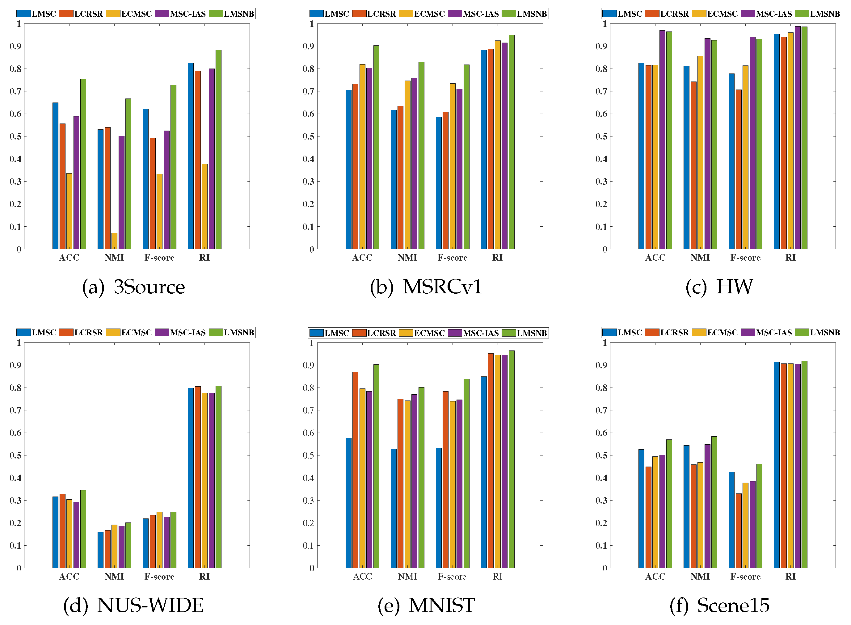
In our experiments, the codes for the compared algorithms are given by the authors, and the parameters are tuned to the optimal performance. For our algorithm, the input data samples are normalized to unit l 2 norm. Similar to [34], we set the dimension K of the latent representation H as 100 for all datasets. As for similarity matrix S, we set the number of the neighborhood as 6 for all datasets, and the bandwidth parameter σ equals to the mean of the Euclidean distances between every two data points. Now, we only need to tune the parameter λ , α and β , which are all searched from the candidate set { 2 2 , 2 0 , 2 2 , 2 4 , 2 6 , 2 8 , 2 10 } . We select the parameters corresponding to the optimal performances for each dataset (see Table 2 for a detail). For the optimal parameters, we repeat each algorithm 30 times and report the means and standard deviations in Table 3. Moreover, we also plot the histograms of clustering performance on six datasets for a better visualization, see Figure 2.
In Table 3, the best results are marked in bold, while the second best results are represented by the underline values. We can observe that LMSNB achieves better performance compared with LMSC, LCRSR, ECMSC and MSC_IAS in most cases.
To be specific, for the results on textual dataset 3Source, our proposed approach achieves 10.51 % , 13.64 % , 10.72 % and 5.79 % average improvements over the most competitive algorithm LMSC in terms of ACC, NMI, F-score and RI, respectively. For most of the image datasets, our LMSNB achieves high clustering accuracy as well as small standard deviations. Taking MSRCv1 for an example, the average ACC and standard deviation are 90.30 % and 0.61 % , respectively. Our LMSNB also gets the similar clustering results on MNIST. For the results on Scene15, LMSNB achieves 4.45 % improvement compared with LMSC in terms of ACC. The clustering results on NUS-WIDE are generally poor for all the compared algorithms, however, LMSNB achieves improvements around 3.74 % and 5.32 % in terms of ACC and NMI compared with the second best method LCRSR. On HW dataset, both MSC_IAS and LMSNB produce encouraging results. Our LMSNB performs only 0.48 % , 0.82 % , 0.89 % and 0.18 % lower than MSC_IAS in terms of ACC, NMI, F-score and RI, respectively, which are negligible differences.
On the whole, our LMSNB is outperformed with the compared algorithms for most of the datasets we used. The compared algorithm MSC_IAS and LMSC are proposed based on the latent intact space, however, MSC_IAS gains better results than LMSC in most cases. The reason may be that the former considers the local geometry, i.e., the intactness-aware similarity in MSC_IAS is learned by the graph regularization. Further, the superior of our algorithm is that LMSNB not only preseves the local geometry deploying the graph regularization, but captures the global information by adding the block diagonal constraint.

5.5. Parameter Sensitivity Analysis

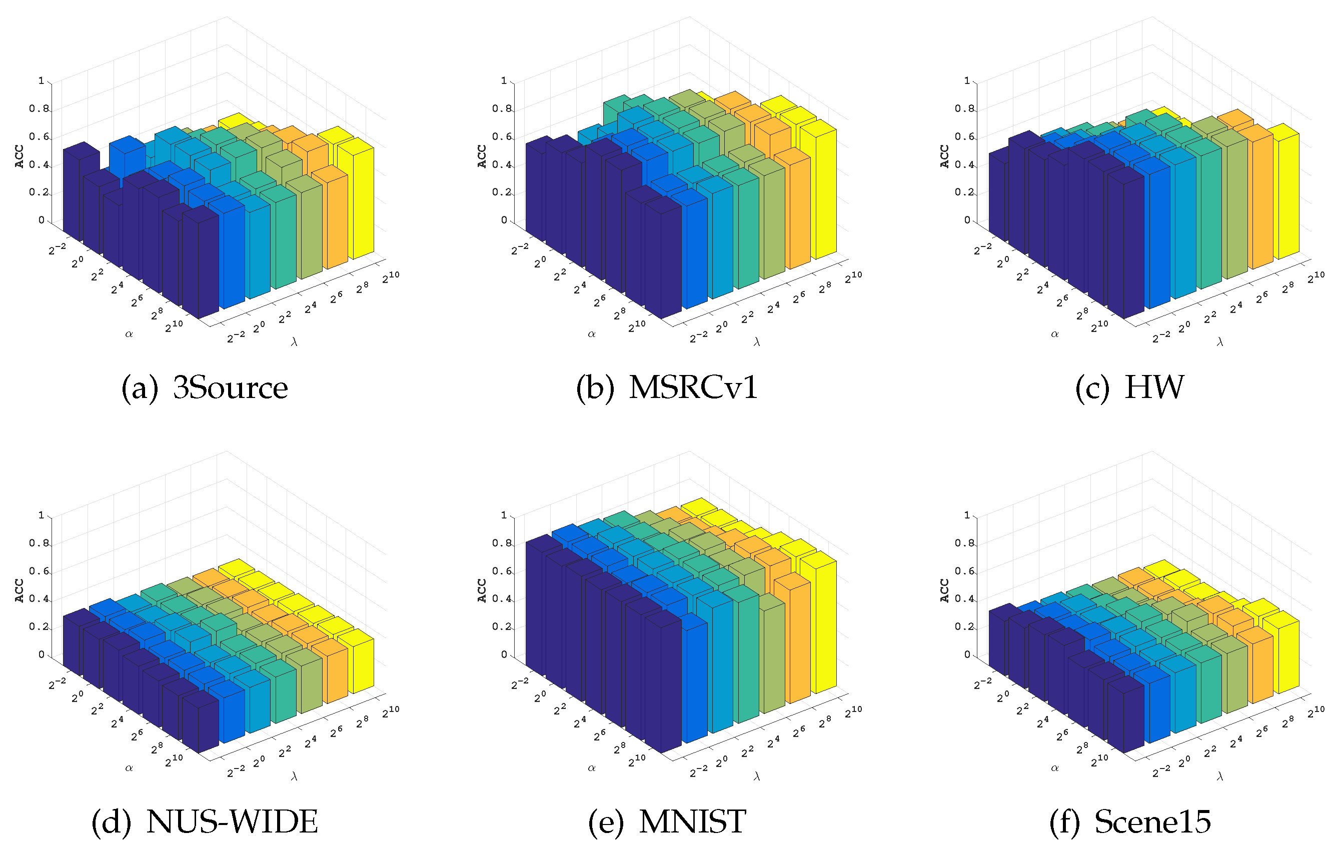
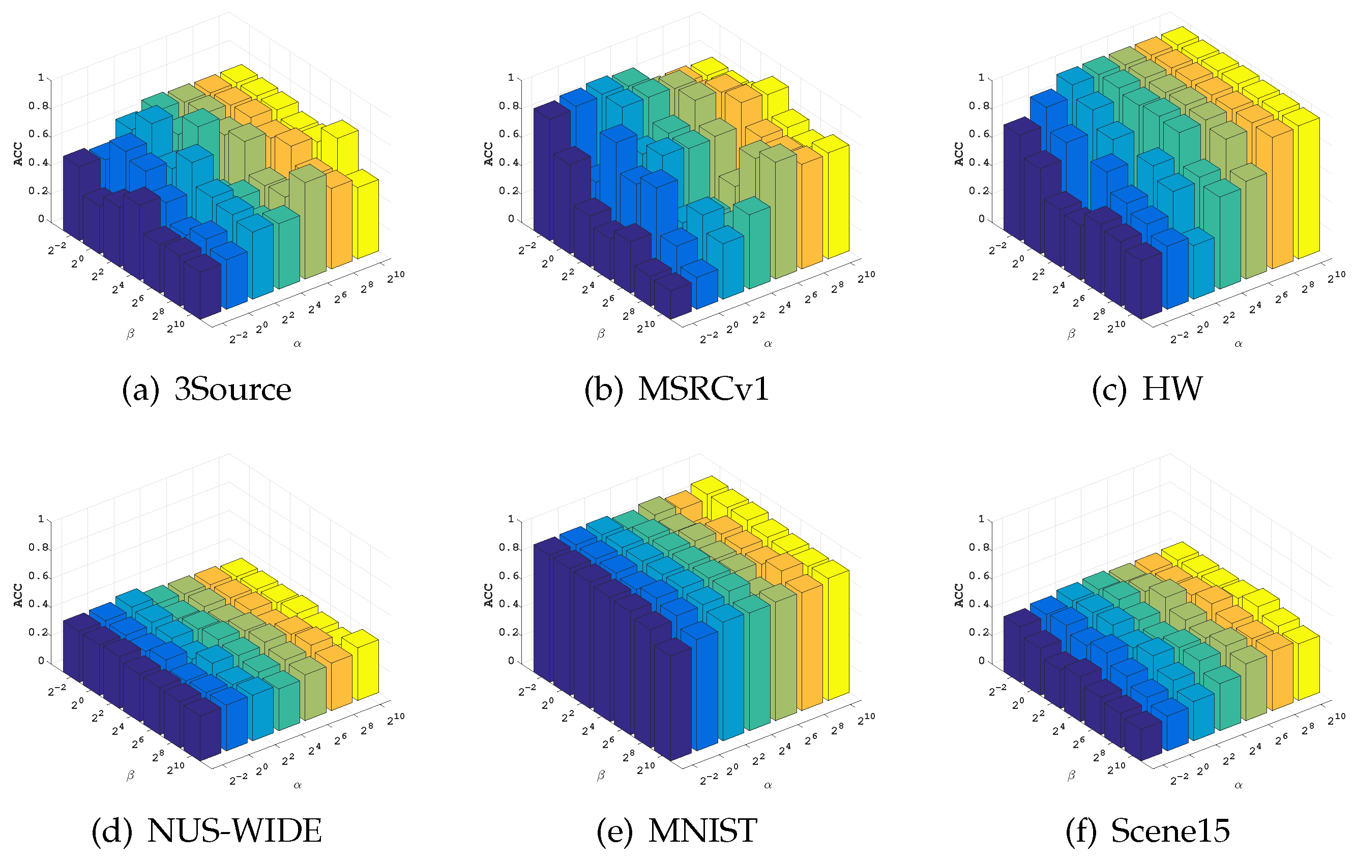
In this part, we show the sentivity analysis of different parameters. There are three tuning parameters λ , α and β in our final model (11). So, we tend to fix one and tune the others. Firstly, we tune λ { 2 2 , 2 0 , 2 2 , 2 4 , 2 6 , 2 8 , 2 10 } and α { 2 2 , 2 0 , 2 2 , 2 4 , 2 6 , 2 8 , 2 10 } when β is fixed to 1. Figure 3 shows that how the ACC changes with varying λ and α when β = 1 . Next, we fix λ = 1 , and tune the α { 2 2 , 2 0 , 2 2 , 2 4 , 2 6 , 2 8 , 2 10 } and β { 2 2 , 2 0 , 2 2 , 2 4 , 2 6 , 2 8 , 2 10 } . Figure 4 shows that how the ACC changes with varying α and β when λ = 1 .
From Figure 3, we can see that our method maintains relatively stable clustering performance over a wide range under most of the datasets we used. Specifically, for NUS-WIDE, MNIST and Scene15, our algorithm supplies a good performance on all the parameters we used. For 3Source and MSRCv1, the ACC performance would be better when the parameter α takes the middle value of its range. As for HW, a larger α will lead to the better results for our algorithm.
From Figure 4, our algorithm performs the relatively stable clustering results on NUS-WIDE and MNIST dataset. For 3Source, HW and Scene15, we can observe that a larger α may produce the better clustering results, and a smaller β also performs the better clustering results.

5.6. Ablation Study

In this section, we will investigate the effectiveness of the block diagonal constraint V V T k . We remove the k-block diagonal constraint term in model (10) as comparative experiment (LMSN) and show the results in Table 4. We run each experiment 30 times and then use t-test at 0.05 significance level to illustrate the statistical significance of the performance produced by LMSNB and LMSN.
From Table 4, we can observe that LMSNB gains better clustering results than LMSN in most of the datasets we used. In particular, our algorithm LMSNB achieves nearly 9 % promotion on MNIST dataset due to the block-diagonal constraint. In a word, the k-block diagonal constraint V V T k can be an effecitve constraint and lead to better results in most cases.

5.7. Visualization of V V T

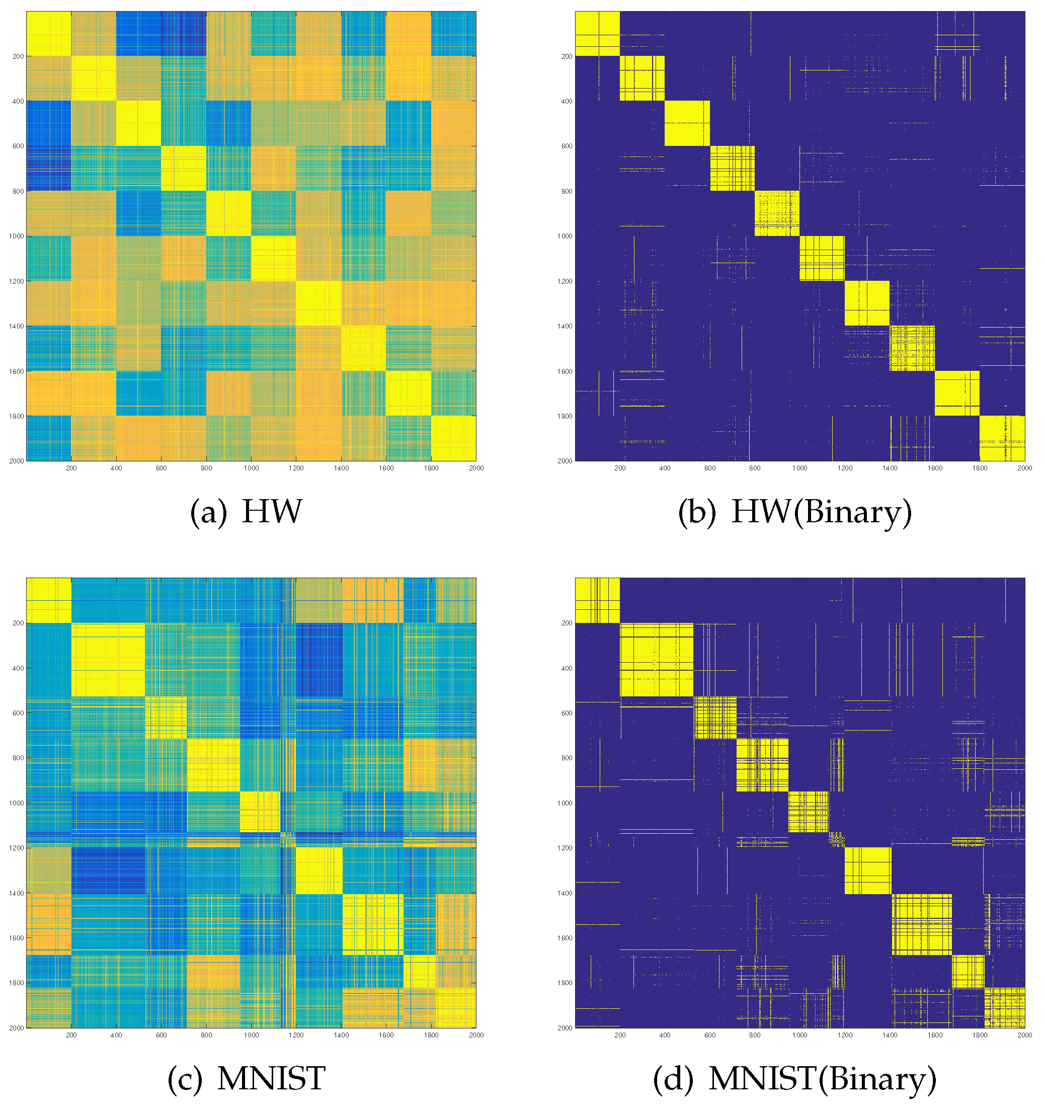
Now, we show the visualization of V V T on HW and MNIST (see Figure 5a,c), where the point tends to be yellow corresponding to a larger value while point rich in blue means a smaller value. It should be noted that the rows of V are permuted according to the true label of the samples. Since the existence of noise or samples located in the boundary of classes, the block diagonal structures are not obvious. Thus, for a better visualization, we also plot the binarized version of V V T on the same datasets (see Figure 5b,d). The binarization of matrix A is defined as follows,
Binary ( A ) i j = 1 , if A i j δ , 0 , otherwise ,
where δ = A ( g = 1 k | C g | 2 ) , A ( t ) represents the t-th maximum element in matrix A. | C g | denotes the number of samples in the g-th cluster. We give a short explanation about the value of δ . Actually, we hope that the number of nonzero elements in Binary ( V V T ) for g-th cluster equals to the square of the size of samples in the same cluster, i.e., | C g | 2 . Then, threshold parameter δ can be defined as the above. From Figure 5b,d, we can observe that V V T indeed owns the block diagonal structure on the two given datasets. Based on this fact, it’s reasonable to impose the k-block diagonal constraint on V V T .

5.8. Time Analysis

In this section, we show the time consumptions of each algorithm, see Table 5. From Table 5, we can see that the speed of our LMSNB is faster than LMSC and ECMSC on most of datasets, but usually slower than LCRSR and MSC_IAS. It should be noted that the time complexity of LMSNB is O ( N 2 k + i = 1 v m i 3 + K 3 ) , which is cubic to m i (the number of features in i-th views). So when M is large, our LMSNB would cost too much time. Take 3Source for an example, although it contains only 169 samples, the numbers of features for three views are 3560, 3631 and 3068, respectively. Thus our algorithm has a longer time consuming.

6. Conclusions

In this paper, we propose an algorithm named latent multi-view semi-nonnegative matrix factorization with block diagonal constraint (LMSNB). Based on Section 5, k-block diagonal structure is usually found in most of datasets. Thus, the assumption of k-block diagonal constraint V V T k is reasonable. It can capture the global structure of the original data and lead to improved clustering performance. Moreover, multi-view latent representation learning, Semi-NMF and graph regularization are utilized to get a shared low-dimensional representation which captures the local geometry. Thus, our model LMSNB enable to produce a new representation which captures the global and local geometry. Experiment results on six multi-view datasets demonstrate the effectiveness of our algorithm.
There are two limitations for our LMSNB. First, for some datasets with high dimension, the time consuming of our algorithm is large. Second, there are three trade-off parameters need to be tuned in our model, which is a barrier for the real applications.
There are also several directions for our future work. First, however it’s unreasonable to set the dimension K as 100 for some datasets (since the constraint P ( i ) P ( i ) T = I ( i ) ), the promising results are still obtained, such as MSRCv1. We will try to explain it in our future work. Second, noticed that the importance of different views are ignored in our model, we will design a framework that considers the weight of different views. Finally, we are also interested in extending our model to semi-supervised tasks.

Author Contributions

Conceptualization, writing—original draft preparation, L.Y.; methodology, writing—review and editing, X.Y.; investigation, writing—review and editing, Z.X.; supervision, methodology, Y.M. All authors have read and agreed to the published version of the manuscript.

Funding

This work is supported by the Natural Science Foundation of China (11501435, 61976130), Natural Science Foundation of Shaanxi Province (2022KRM170), key research and development projects of Shaanxi Province (2018KW-021).

Institutional Review Board Statement

Not applicable.

Informed Consent Statement

Not applicable.

Data Availability Statement

Our code will be published at https://github.com/exclusive1016 (accessed on 10 September 2022).

Acknowledgments

The authors wish to gratefully acknowledge the anonymous reviewers for the constructive comments of this paper.

Conflicts of Interest

The authors declare no conflict of interest.

Abbreviations

The following abbreviations are used in this manuscript:
MVCmulti-view clustering
SSCSparse Subspace Clustering
LRRLow Rank Representation
NMFNonnegative Matrix Factorization
SVDSingular Value Decomposition
KKTKarush–Kuhn–Tucker

Appendix A. The Proof of Theorem 4

In this appendix, we prove Theorem 4 is correct. Our proof will start from an auxiliary function.
Definition A1. 
G ( h , h ) is said to be an auxiliary function for F ( h ) if the conditions
G ( h , h ) F ( h ) , G ( h , h ) = F ( h ) ,
are satisfied.
Lemma A1. 
If G is an auxiliary function of F, then F is nonincreasing under the update
h ( t + 1 ) = argmin h G ( h , h ( t ) ) .
Proof. 
F ( h ( t + 1 ) ) G ( h ( t + 1 ) , h ( t ) ) G ( h ( t ) , h ( t ) ) = F ( h ( t ) ) .
Applying Equation (4) into problem (11), the objective function (11) can be rewritten as follows
O = E 2 , 1 + λ H U V T F 2 + α Tr ( V T L V ) + β V V T , w 1 T W
Considering any element V i j in V, we use F i j to denote the part of O , which is only relevant to V i j . It’s easy to get the following equations:
F i j = O V i j = 2 λ V U T U 2 λ H T U + 2 α L V + β W ˜ T V + β W ˜ V i j ,
F i j = 2 λ ( U T U ) j j + ( 2 α L + β W ˜ T + β W ˜ ) i i ,
where W ˜ = w 1 T W . The following work is to find an auxiliary function for F i j .
Lemma A2. 
Function
G ( V i j , V i j ( t ) ) = F i j ( V i j ( t ) ) + F i j ( V i j ( t ) ) ( V i j V i j ( t ) ) + B i j 2 V i j ( t ) ( V i j V i j ( t ) ) 2
is an auxiliary function for F i j , where
B = 2 λ ( H T U ) + 2 λ V ( t ) ( U T U ) + + 2 α D V ( t ) + β w 1 T + 1 w T V ( t ) + 2 β W V ( t ) .
Proof. 
Firstly, G ( V i j , V i j ) = F i j ( V i j ) is obvious, we only show that G ( V i j , V i j ( t ) ) F i j ( V i j ) . By (A3) and (A4), we compare the Taylor series expension of F i j ( V i j ) ,
F i j ( V i j ) = F i j ( V i j ( t ) ) + F i j ( V i j ( t ) ) ( V i j V i j ( t ) ) + 1 2 2 λ ( U T U ) j j + ( 2 α L + β W ˜ T + β W ˜ ) i i ( V i j V i j ( t ) ) 2 ,
with (A5) to find that G ( V i j , V i j ( t ) ) F i j ( V i j ) is equivalent to
2 λ ( H T U ) + 2 λ V ( t ) ( U T U ) + + 2 α D V ( t ) + β w 1 T + 1 w T V ( t ) + 2 β W V ( t ) i j 2 V i j ( t ) λ U T U j j + ( α L + 1 2 β W ˜ T + 1 2 β W ˜ ) i i
Then we have
2 λ V ( t ) ( U T U ) + i j = 2 λ l = 1 K V i l ( t ) ( U T U ) l j + 2 λ V i j ( t ) ( U T U ) j j ,
( 2 α D V ( t ) ) i j = 2 α d = 1 N D i d V d j ( t ) 2 α D i i V i j ( t ) 2 α ( D S ) i i V i j ( t ) = 2 α L i i V i j ( t ) ,
( β w 1 T V ( t ) ) i j = β d = 1 N w 1 T i d V d j ( t ) β w 1 T i i V i j ( t ) β w 1 T W i i V i j ( t ) = β W ˜ i i V i j ( t ) ,
For (A10), the second inequality holds since the diagonal elements of the positive semi-definite matrix W are all nonnegative. Replacing w 1 T in (A10) by 1 w T , we have
( β 1 w T V ( t ) ) i j β W ˜ i i T V i j ( t ) .
Note that λ ( H T U ) i j and β ( W V ( t ) ) i j are nonnegative, then, (A7) holds and G ( V i j , V i j ( t ) ) F i j ( V i j ) .
Now, we can demonstrate the validity of Theorem 4.
Proof of Theorem 4. 
Since G ( V , V ( t ) ) in Lemma A2 is an auxiliary function of F i j , we can take the partial derivative of (A1) with respect to V i j and set it to zero. Then, we have
V i j ( t + 1 ) = V i j ( t ) ( 2 λ ( H T U ) + + 2 λ V ( t ) ( U T U ) + 2 α S V + 2 β W + V ( t ) ) i j 2 λ ( H T U ) + 2 λ V ( t ) ( U T U ) + + 2 α D V ( t ) + β w 1 T + 1 w T V ( t ) + 2 β W V ( t ) i j .
This is the end of the proof. □

References

  1. Hartigan, J.A.; Wong, M.A. Algorithm AS 136: A k-means clustering algorithm. J. R. Stat. Soc. Ser. C Appl. Stat. 1979, 28, 100–108. [Google Scholar] [CrossRef]
  2. Von Luxburg, U. A tutorial on spectral clustering. Stat. Comput. 2007, 17, 395–416. [Google Scholar] [CrossRef]
  3. Ehsan Elhamifar, R.V. Sparse subspace clustering. In Proceedings of the 2009 IEEE Conference on Computer Vision and Pattern Recognition (CVPR), Miami, FL, USA, 20–25 June 2009; Volume 6, pp. 2790–2797. [Google Scholar]
  4. Liu, G.; Lin, Z.; Yan, S.; Sun, J.; Yu, Y.; Ma, Y. Robust recovery of subspace structures by low-rank representation. IEEE Trans. Pattern Anal. Mach. Intell. 2012, 35, 171–184. [Google Scholar] [CrossRef] [Green Version]
  5. Saberi-Movahed, F.; Rostami, M.; Berahmand, K.; Karami, S.; Tiwari, P.; Oussalah, M.; Band, S.S. Dual Regularized Unsupervised Feature Selection Based on Matrix Factorization and Minimum Redundancy with application in gene selection. Knowl.-Based Syst. 2022, 256, 109884. [Google Scholar] [CrossRef]
  6. Rostami, M.; Oussalah, M.; Farrahi, V. A Novel Time-Aware Food Recommender-System Based on Deep Learning and Graph Clustering. IEEE Access 2022, 10, 52508–52524. [Google Scholar] [CrossRef]
  7. Caruso, G.; Gattone, S.A.; Balzanella, A.; Di Battista, T. Cluster Analysis: An Application to a Real Mixed-Type Data Set. In Models and Theories in Social Systems; Springer International Publishing: Cham, Switerland, 2019; pp. 525–533. [Google Scholar] [CrossRef]
  8. Eisen, M.B.; Spellman, P.T.; Brown, P.O.; Botstein, D. Cluster analysis and display of genome-wide expression patterns. Proc. Natl. Acad. Sci. USA 1998, 95, 14863–14868. [Google Scholar] [CrossRef] [Green Version]
  9. Takita, M.; Matsumoto, S.; Noguchi, H.; Shimoda, M.; Chujo, D.; Itoh, T.; Sugimoto, K.; SoRelle, J.A.; Onaca, N.; Naziruddin, B.; et al. Cluster analysis of self-monitoring blood glucose assessments in clinical islet cell transplantation for type 1 diabetes. Diabetes Care 2011, 34, 1799–1803. [Google Scholar] [CrossRef] [Green Version]
  10. Azadifar, S.; Rostami, M.; Berahmand, K.; Moradi, P.; Oussalah, M. Graph-based relevancy-redundancy gene selection method for cancer diagnosis. Comput. Biol. Med. 2022, 147, 105766. [Google Scholar] [CrossRef]
  11. Bickel, S.; Scheffer, T. Multi-View Clustering. In Proceedings of the Fourth IEEE International Conference on Data Mining (ICDM’04), Brighton, UK, 1–4 November 2004; pp. 19–26. [Google Scholar]
  12. Chao, G.; Sun, S.; Bi, J. A survey on multi-view clustering. IEEE Trans. Artif. Intell. 2021, 2, 146–168. [Google Scholar] [CrossRef] [PubMed]
  13. Kang, H.; Xia, L.; Yan, F.; Wan, Z.; Shi, F.; Yuan, H.; Jiang, H.; Wu, D.; Sui, H.; Zhang, C.; et al. Diagnosis of coronavirus disease 2019 (COVID-19) with structured latent multi-view representation learning. IEEE Trans. Med. Imaging 2020, 39, 2606–2614. [Google Scholar] [CrossRef]
  14. Fu, L.; Lin, P.; Vasilakos, A.V.; Wang, S. An overview of recent multi-view clustering. Neurocomputing 2020, 402, 148–161. [Google Scholar] [CrossRef]
  15. Wang, R.; Nie, F.; Wang, Z.; Hu, H.; Li, X. Parameter-free weighted multi-view projected clustering with structured graph learning. IEEE Trans. Knowl. Data Eng. 2019, 32, 2014–2025. [Google Scholar] [CrossRef]
  16. Wang, S.; Liu, X.; Zhu, E.; Tang, C.; Liu, J.; Hu, J.; Xia, J.; Yin, J. Multi-view Clustering via Late Fusion Alignment Maximization. In Proceedings of the IJCAI, Macao, China, 10–16 August 2019; pp. 3778–3784. [Google Scholar]
  17. Peng, X.; Huang, Z.; Lv, J.; Zhu, H.; Zhou, J.T. COMIC: Multi-view clustering without parameter selection. In Proceedings of the International Conference on Machine Learning, PMLR, Long Beach, CA, USA, 9–15 June 2019; pp. 5092–5101. [Google Scholar]
  18. Nie, F.; Shi, S.; Li, X. Auto-weighted multi-view co-clustering via fast matrix factorization. Pattern Recognit. 2020, 102, 107207. [Google Scholar] [CrossRef]
  19. Li, X.; Zhang, H.; Wang, R.; Nie, F. Multi-view clustering: A scalable and parameter-free bipartite graph fusion method. IEEE Trans. Pattern Anal. Mach. Intell. 2020, 44, 330–344. [Google Scholar] [CrossRef]
  20. Kumar, A.; Daumé, H. A co-training approach for multi-view spectral clustering. In Proceedings of the 28th International Conference on Machine Learning (ICML-11), Bellevue, WA, USA, 28 June–2 July 2011; pp. 393–400. [Google Scholar]
  21. Lee, C.; Liu, T. Guided co-training for multi-view spectral clustering. In Proceedings of the 2016 IEEE International Conference on Image Processing (ICIP), Phoenix, AZ, USA, 25–28 September 2016; pp. 4042–4046. [Google Scholar]
  22. Lu, R.; Liu, J.; Wang, Y.; Xie, H.; Zuo, X. Auto-encoder based co-training multi-view representation learning. In Advances in Knowledge Discovery and Data Mining, Proceedings of the 23rd Pacific-Asia Conference, PAKDD 2019, Macau, China, 14–17 April 2019; Springer: Cham, Switerland, 2019; pp. 119–130. [Google Scholar]
  23. Zhao, B.; Kwok, J.T.; Zhang, C. Multiple kernel clustering. In Proceedings of the 2009 SIAM International Conference on Data Mining, Sparks, NV, USA, 30 April–2 May 2009; pp. 638–649. [Google Scholar]
  24. Sun, M.; Wang, S.; Zhang, P.; Liu, X.; Guo, X.; Zhou, S.; Zhu, E. Projective Multiple Kernel Subspace Clustering. IEEE Trans. Multimed. 2021, 24, 2567–2579. [Google Scholar] [CrossRef]
  25. Nie, F.; Li, J.; Li, X. Parameter-free auto-weighted multiple graph learning: A framework for multiview clustering and semi-supervised classification. In Proceedings of the IJCAI, New York, NY, USA, 9–15 July 2016; pp. 1881–1887. [Google Scholar]
  26. Hussain, S.F.; Mushtaq, M.; Halim, Z. Multi-view document clustering via ensemble method. J. Intell. Inf. Syst. 2014, 43, 81–99. [Google Scholar] [CrossRef]
  27. Nie, F.; Li, J.; Li, X. Self-weighted Multiview Clustering with Multiple Graphs. In Proceedings of the IJCAI, Melbourne, Australia, 19–25 August 2017; pp. 2564–2570. [Google Scholar]
  28. Zhang, C.; Fu, H.; Hu, Q.; Cao, X.; Xie, Y.; Tao, D.; Xu, D. Generalized latent multi-view subspace clustering. IEEE Trans. Pattern Anal. Mach. Intell. 2018, 42, 86–99. [Google Scholar] [CrossRef]
  29. Zhang, P.; Liu, X.; Xiong, J.; Zhou, S.; Zhao, W.; Zhu, E.; Cai, Z. Consensus one-step multi-view subspace clustering. IEEE Trans. Knowl. Data Eng. 2020, 34, 4676–4689. [Google Scholar] [CrossRef]
  30. Gao, H.; Nie, F.; Li, X.; Huang, H. Multi-view subspace clustering. In Proceedings of the IEEE International Conference on Computer Vision, Santiago, Chile, 7–13 December 2015; pp. 4238–4246. [Google Scholar]
  31. Brbić, M.; Kopriva, I. Multi-view low-rank sparse subspace clustering. Pattern Recognit. 2018, 73, 247–258. [Google Scholar] [CrossRef]
  32. Wang, X.; Guo, X.; Lei, Z.; Zhang, C.; Li, S.Z. Exclusivity-consistency regularized multi-view subspace clustering. In Proceedings of the 2017 IEEE Conference on Computer Vision and Pattern Recognition (CVPR), Honolulu, HI, USA, 21–26 July 2017; pp. 923–931. [Google Scholar]
  33. Xu, C.; Tao, D.; Xu, C. Multi-view intact space learning. IEEE Trans. Pattern Anal. Mach. Intell. 2015, 37, 2531–2544. [Google Scholar] [CrossRef] [Green Version]
  34. Zhang, C.; Hu, Q.; Fu, H.; Zhu, P.; Cao, X. Latent multi-view subspace clustering. In Proceedings of the 2017 IEEE Conference on Computer Vision and Pattern Recognition (CVPR), Honolulu, HI, USA, 21–26 July 2017; pp. 4279–4287. [Google Scholar]
  35. Lin, K.; Wang, C.; Meng, Y.; Zhao, Z. Multi-view unit intact space learning. In Knowledge Science, Engineering and Management, Proceedings of the 10th International Conference, KSEM 2017, Melbourne, VIC, Australia, 19–20 August 2017; Springer: Cham, Switzerland, 2017; pp. 211–223. [Google Scholar]
  36. Huang, L.; Chao, H.Y.; Wang, C.D. Multi-view intact space clustering. Pattern Recognit. 2019, 86, 344–353. [Google Scholar] [CrossRef]
  37. Tao, H.; Hou, C.; Qian, Y.; Zhu, J.; Yi, D. Latent complete row space recovery for multi-view subspace clustering. IEEE Trans. Image Process. 2020, 29, 8083–8096. [Google Scholar] [CrossRef]
  38. Chen, M.; Huang, L.; Wang, C.; Huang, D. Multi-view clustering in latent embedding space. In Proceedings of the AAAI Conference on Artificial Intelligence, New York, NY, USA, 7–12 February 2020; Volume 34, pp. 3513–3520. [Google Scholar]
  39. Xie, D.; Gao, Q.; Wang, Q.; Zhang, X.; Gao, X. Adaptive latent similarity learning for multi-view clustering. Neural Netw. 2020, 121, 409–418. [Google Scholar] [CrossRef] [PubMed]
  40. Wang, X.; Lei, Z.; Guo, X.; Zhang, C.; Shi, H.; Li, S.Z. Multi-view subspace clustering with intactness-aware similarity. Pattern Recognit. 2019, 88, 50–63. [Google Scholar] [CrossRef]
  41. Lee, D.D.; Seung, H.S. Learning the parts of objects by non-negative matrix factorization. Nature 1999, 401, 788–791. [Google Scholar] [CrossRef]
  42. Cai, D.; He, X.; Han, J.; Huang, T. Graph regularized non-negative matrix factorization for data representation. IEEE Trans. Pattern Anal. Mach. Intell. 2011, 33, 1548–1560. [Google Scholar]
  43. Ding, C.H.; Li, T.; Jordan, M.I. Convex and semi-nonnegative matrix factorizations. IEEE Trans. Pattern Anal. Mach. Intell. 2008, 32, 45–55. [Google Scholar] [CrossRef] [Green Version]
  44. Liu, J.; Wang, C.; Gao, J.; Han, J. Multi-view clustering via joint nonnegative matrix factorization. In Proceedings of the 2013 SIAM International Conference on Data Mining, Austin, TX, USA, 2–4 May 2013; pp. 252–260. [Google Scholar]
  45. Hidru, D.; Goldenberg, A. EquiNMF: Graph Regularized Multiview Nonnegative Matrix Factorization. arXiv 2014, arXiv:1409.4018. [Google Scholar]
  46. Rai, N.; Negi, S.; Chaudhury, S.; Deshmukh, O. Partial multi-view clustering using graph regularized NMF. In Proceedings of the 2016 23rd International Conference on Pattern Recognition (ICPR), Cancun, Mexico, 4–8 December 2016; pp. 2192–2197. [Google Scholar]
  47. Zhao, H.; Ding, Z.; Fu, Y. Multi-view clustering via deep matrix factorization. In Proceedings of the Thirty-First AAAI Conference on Artificial Intelligence, San Francisco, CA, USA, 4–9 February 2017; pp. 2921–2927. [Google Scholar]
  48. Kullback, S.; Leibler, R.A. On information and sufficiency. Ann. Math. Stat. 1951, 22, 79–86. [Google Scholar] [CrossRef]
  49. Cichocki, A.; Lee, H.; Kim, Y.; Choi, S. Non-negative matrix factorization with α-divergence. Pattern Recognit. Lett. 2008, 29, 1433–1440. [Google Scholar] [CrossRef]
  50. Févotte, C.; Idier, J. Algorithms for nonnegative matrix factorization with the β-divergence. Neural Comput. 2011, 23, 2421–2456. [Google Scholar] [CrossRef]
  51. Feng, J.; Lin, Z.; Xu, H.; Yan, S. Robust subspace segmentation with block-diagonal prior. In Proceedings of the IEEE Conference on Computer Vision and Pattern Recognition, Columbus, OH, USA, 23–28 June 2014; pp. 3818–3825. [Google Scholar]
  52. Lu, C.; Feng, J.; Lin, Z.; Mei, T.; Yan, S. Subspace clustering by block diagonal representation. IEEE Trans. Pattern Anal. Mach. Intell. 2018, 41, 487–501. [Google Scholar] [CrossRef] [PubMed] [Green Version]
  53. Belkin, M.; Niyogi, P. Laplacian eigenmaps and spectral techniques for embedding and clustering. Adv. Neural Inf. Process. Syst. 2001, 14, 585–591. [Google Scholar]
  54. Dattorro, J. Convex Optimization & Euclidean Distance Geometry; Lulu: Durham, NC, USA, 2019. [Google Scholar]
  55. Huang, J.; Nie, F.; Huang, H. Spectral rotation versus k-means in spectral clustering. In Proceedings of the AAAI Conference on Artificial Intelligence, Bellevue, WA, USA, 14–18 July 2013; Volume 27. [Google Scholar]
  56. Yang, J.; Yin, W.; Zhang, Y.; Wang, Y. A fast algorithm for edge-preserving variational multichannel image restoration. SIAM J. Imaging Sci. 2009, 2, 569–592. [Google Scholar] [CrossRef]
  57. Chua, T.; Tang, J.; Hong, R.; Li, H.; Luo, Z.; Zheng, Y. Nus-wide: A real-world web image database from National University of Singapore. In Proceedings of the ACM International Conference on Image and Video Retrieval, Santorini Island, Greece, 8–10 July 2009; pp. 1–9. [Google Scholar]
  58. Lazebnik, S.; Schmid, C.; Ponce, J. Beyond bags of features: Spatial pyramid matching for recognizing natural scene categories. In Proceedings of the 2006 IEEE Computer Society Conference on Computer Vision and Pattern Recognition (CVPR’06), New York, NY, USA, 17–22 June 2006; Volume 2, pp. 2169–2178. [Google Scholar]
  59. Dai, D.; Van Gool, L. Ensemble projection for semi-supervised image classification. In Proceedings of the IEEE International Conference on Computer Vision, Sydney, Australia, 1–8 December 2013; pp. 2072–2079. [Google Scholar]
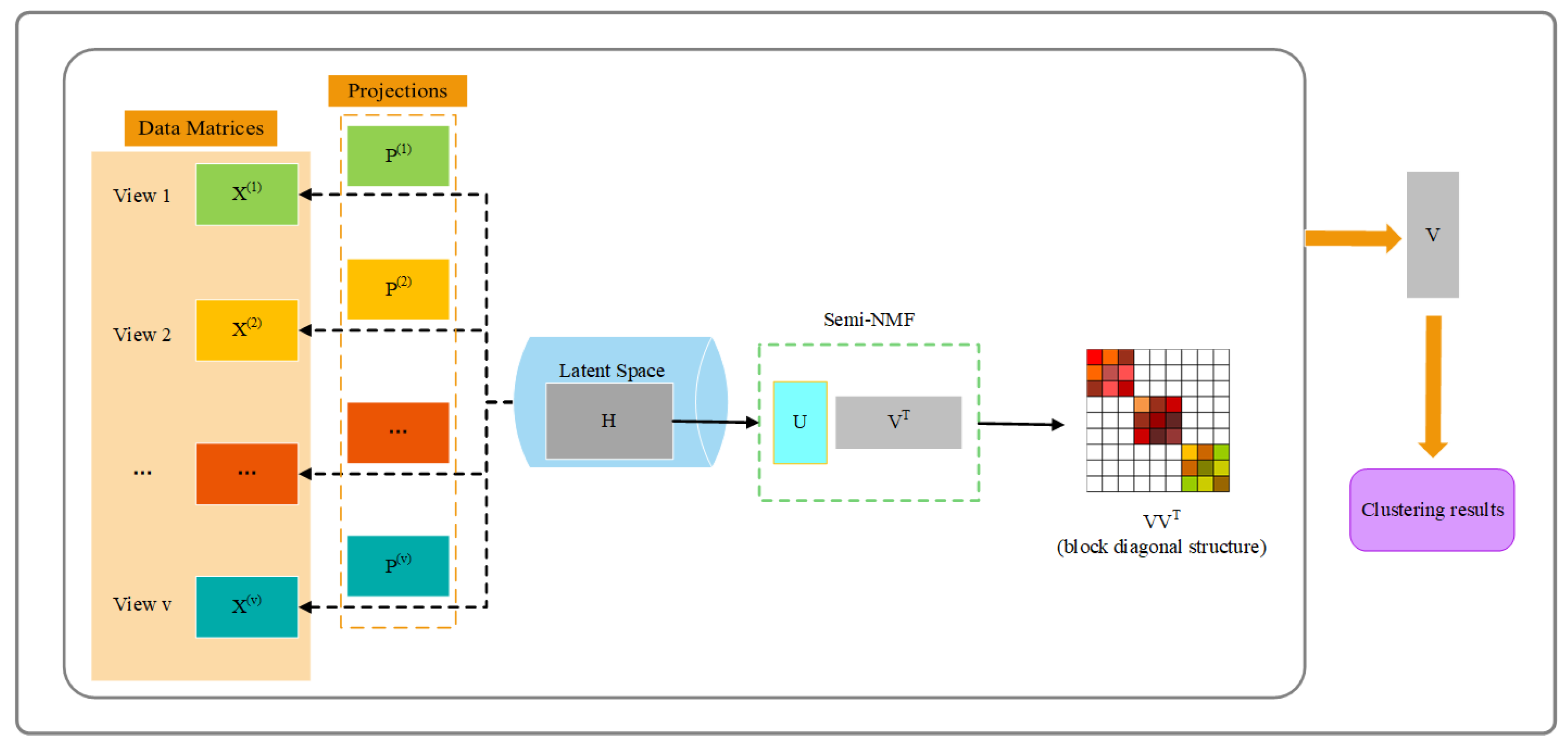
Figure 1. The general framework of our proposed approach. X ( i ) and P ( i ) represent the data matrix and projection matrix from the i-view, respectively. H denotes the latent representation of multi-view data. The basis matrix U in Semi-NMF is free while the encoding matrix V is constrainted to be nonnegative. We assume that V V T is a k-block diagonal matrix in our model.
Axioms 11 00722 g001
Figure 2. The histograms of clustering performance on different datasets.
Axioms 11 00722 g002
Figure 3. The ACC performance for different λ and α (when β = 1 ).
Axioms 11 00722 g003
Figure 4. The ACC performance for different α and β (when λ = 1 ).
Axioms 11 00722 g004
Figure 5. Block diagonal structure visualization of V V T . (a,c) are the original V V T of HW and MNIST, respectively. (b,d) are the binarized V V T of HW and MNIST, respectively.
Axioms 11 00722 g005
Table 1. Statistics of the six datasets.
DatasetsSamplesViewsClusters
3Source16936
MSRCv121057
HW2000610
NUS-WIDE160068
MNIST2000310
Scene154485315
Table 2. The optimal values of the three parameters.
Parameter3SourceMSRCv1HWNUS-WIDEMNISTScene15
λ 2 4 2 2 2 2 2 2 2 0 2 2
α 2 4 2 4 2 10 2 0 2 4 2 2
β 2 0 2 0 2 0 2 0 2 0 2 0
Table 3. Clustering performance on six datasets (mean ± standard deviation %).
DatasetsMethodsACCNMIF-ScoreRI
3SourseLMSC 64.97 ± 3.00 ̲ 53.07 ± 1.94 62.09 ± 3.59 ̲ 82.47 ± 2.11 ̲
LCRSR 55.56 ± 0.18 53.94 ± 0.93 ̲ 49.18 ± 0.92 78.91 ± 0.42
ECMSC 33.61 ± 2.88 7.21 ± 1.22 33.31 ± 3.35 37.68 ± 10.96
MSC_IAS 58.95 ± 6.92 50.20 ± 5.43 52.42 ± 6.00 79.96 ± 2.53
LMSNB 75 . 48 ± 3 . 89 66 . 71 ± 3 . 17 72 . 81 ± 3 . 39 88 . 26 ± 1 . 34
MSRCv1LMSC 70.49 ± 5.86 61.69 ± 6.04 58.59 ± 6.58 88.28 ± 1.82
LCRSR 73.16 ± 0.26 63.41 ± 0.64 60.78 ± 0.43 88.80 ± 0.12
ECMSC 81.90 ± 0.00 ̲ 74.62 ± 0.00 73.47 ± 0.00 ̲ 92.52 ± 0.00 ̲
MSC_IAS 80.24 ± 2.04 75.92 ± 1.33 ̲ 70.97 ± 1.49 91.53 ± 0.44
LMSNB 90 . 30 ± 0 . 61 83 . 04 ± 0 . 71 81 . 76 ± 0 . 99 94 . 86 ± 0 . 29
HWLMSC 82.53 ± 5.48 81.27 ± 1.84 77.86 ± 3.36 95.40 ± 0.78
LCRSR 81.52 ± 4.29 74.24 ± 1.76 70.75 ± 3.12 94.12 ± 0.66
ECMSC 81.60 ± 0.00 85.55 ± 0.00 81.39 ± 0.00 96.09 ± 0.00
MSC_IAS 96 . 96 ± 0 . 10 93 . 41 ± 0 . 17 94 . 05 ± 0 . 19 98 . 82 ± 0 . 04
LMSNB 96.48 ± 0.02 ̲ 92.59 ± 0.05 ̲ 93.16 ± 0.05 ̲ 98.64 ± 0.01 ̲
NUS-WIDELMSC 31.66 ± 1.79 15.92 ± 1.14 21.87 ± 1.01 79.83 ± 0.29
LCRSR 32.78 ± 0.52 ̲ 16.66 ± 0.40 23.39 ± 0.30 80.51 ± 0.15 ̲
ECMSC 30.31 ± 0.00 19.13 ± 0.00 ̲ 24 . 95 ± 0 . 00 77.57 ± 0.00
MSC_IAS 29.33 ± 0.75 18.65 ± 0.56 22.59 ± 0.39 77.61 ± 0.35
LMSNB 34 . 53 ± 1 . 63 20 . 15 ± 0 . 91 24.73 ± 0.39 ̲ 80 . 70 ± 0 . 37
MNISTLMSC 57.68 ± 4.63 52.64 ± 7.18 53.24 ± 4.36 84.92 ± 5.37
LCRSR 86.94 ± 0.03 ̲ 74.87 ± 0.07 78.35 ± 0.06 ̲ 95.17 ± 0.01 ̲
ECMSC 79.50 ± 0.00 74.15 ± 0.00 73.97 ± 0.00 94.51 ± 0.00
MSC_IAS 78.27 ± 3.35 76.99 ± 1.62 ̲ 74.63 ± 2.80 94.51 ± 0.72
LMSNB 90 . 28 ± 0 . 12 80 . 10 ± 0 . 19 83 . 82 ± 0 . 21 96 . 39 ± 0 . 05
Scene15LMSC 52.54 ± 2.32 ̲ 54.30 ± 2.19 42.50 ± 2.12 ̲ 91.28 ± 0.42 ̲
LCRSR 44.94 ± 1.58 45.89 ± 0.63 33.02 ± 0.96 90.59 ± 0.14
ECMSC 49.39 ± 2.35 46.84 ± 0.90 37.75 ± 1.14 90.63 ± 0.40
MSC_IAS 50.16 ± 1.39 54.71 ± 0.64 ̲ 38.41 ± 0.83 90.49 ± 0.39
LMSNB 56 . 99 ± 0 . 95 58 . 36 ± 0 . 18 46 . 06 ± 0 . 60 91 . 84 ± 0 . 15
Table 4. The ACC performance of ablation study (mean ± standard deviation %).
DatasetsLMSNBLMSNt-Test
3Sourse 75 . 48 ± 3 . 89 73.22 ± 3.26 Yes
MSRCv1 90 . 30 ± 0 . 61 87.49 ± 1.35 Yes
HW 96.48 ± 0.02 96 . 50 ± 0 . 01 Yes
NUS-WIDE 34.53 ± 1.63 36 . 88 ± 0 . 98 Yes
MNIST 90 . 28 ± 0 . 12 81.78 ± 1.78 Yes
Scene15 56 . 99 ± 0 . 95 54.35 ± 1.79 Yes
The best results are marked in bold.
Table 5. The time consuming of different algorithms.
Methods3SourceMSRCv1HWNUS-WIDEMNISTScene15
LMSC9.413.00552.98278.37620.816253.14
LCRSR2.931.3013.7914.564.98465.73
ECMSC183.042.21158.1497.0653.431476.50
MSC_IAS11.021.0214.9314.7216.3280.34
LMSNB69.401.1227.1517.5830.60306.88
Publisher’s Note: MDPI stays neutral with regard to jurisdictional claims in published maps and institutional affiliations.