Abstract
With the development of technology and the increase of equipment usage intensity, the original support mode of circuit repair, with an ideal model and single objective, is no longer applicable. Therefore, we focus on improving the support mode of circuit repair in this article. First, in this article, we propose three rest strategies, and consider the scheduling optimization of flexible rest for repair teams, for the first time. We build a more scientific and comprehensive mathematical model for the task scheduling of circuit repair. Specifically, this model aims to maximize benefits and minimize risks during scheduling up to a certain moment, taking into account constraints, such as geographic information, resources, etc. Second, in this article, we design three hybrid algorithms, namely, NSGAII-2Opt-DE(N2D), SPEA2-2Opt-DE(S2D) and MOEA/D-2Opt-DE(M2D). Third, in this article, we design a comprehensive evaluation indicator, area. It mainly contributes to evaluation of the convergence speed of the multi-objective optimization algorithms. Finally, extensive computational experiments were conducted to verify the scientificity of the rest strategies, model, algorithms and evaluation indicator proposed in this article. The experimental results showed that our proposed N2D, S2D and M2D outperformed the existing algorithms, in terms of solution quality and convergence speed.
Keywords:
multi-objective optimization; circuit repair; benefits; risks; flexible rest; various repair status MSC:
90-10
1. Introduction
As one of the main methods of equipment maintenance, circuit repair can maintain and restore the functions of equipment by dispatching repair teams to provide services at demand points in different locations.
At present, the task scheduling information of circuit repair is quickly updated, the demand points are widely distributed, the environments change dynamically, and the equipment is complicated [1]. The original support mode of circuit repair, with an ideal model and single objective, is no longer applicable. “Poor equipment integrity and high repair costs” often occur. Therefore, it is very important to allocate resources in a balanced manner, schedule tasks scientifically, transform extensive equipment maintenance support into precise support, give full play to the effectiveness of the support system, and restore the functions of the equipment system in a timely manner.
First, this article proposes three rest strategies, and considers the scheduling optimization of flexible rest for repair teams. We built a more scientific and comprehensive mathematical model for the task scheduling of circuit repair, on the basis of the research in [2]. This model aims to maximize benefits and minimize risks during repair up to a certain moment. We fully considered the facts involved, namely, that the repairable status of various demand points is different, the work efficiencies of various repair teams are different, the changes of work efficiency of various repair teams are different, and the rest time arrangements of various repair teams are different.
Second, this article proposes Reversal-1 and 2 operators for the local search algorithm, 2-Optimization(2-Opt) [3]. Based on multi-objective genetic algorithms, NSGA-II, SPEA2, MOEA/D [4,5,6], combined with Differential Evolution (DE), we propose the following three hybrid algorithms: NSGAII-2Opt-DE(N2D), SPEA2-2Opt-DE(S2D) and MOEA/D-2Opt-DE(M2D).
Third, this article designs a comprehensive evaluation indicator, area. The area can evaluate the convergence and one-sided spread of the sets solved by multi-objective optimization algorithms. It mainly contributes to the evaluation of the convergence speed of the multi-objective optimization algorithms.
Finally, we conducted computational experiments, and used indicators C, S, [7,8,9] and area to evaluate the convergence, distribution, spread and convergence speed of the algorithms. The experimental results verified the scientificity of the rest strategies, model, algorithms and evaluation indicator proposed in this article. Moreover, the experimental results showed that our proposed N2D, S2D and M2D outperformed the existing algorithms, including NSGA-II, SPEA2 and MOEA/D [4,5,6], in terms of solution quality and convergence speed.
The contributions of this article are as follows:
- (1)
- The proposal of three rest strategies, considering, for the first time, the flexible rest of the repair teams in circuit repair.
- (2)
- Research that is compatible with traversal and non-traversal task scheduling.
- (3)
- Distinguishing the repairable status of different demand points, compatible with the repair, to a certain status, in a situation involving a single faulty piece of equipment and in a system composed of multiple pieces of equipment.
- (4)
- The multi-layer coding method is adopted and three multi-objective hybrid genetic algorithms are designed, which are compatible with the task scheduling of a single repair team and multiple repair teams. The hybrid algorithms have good solution qualities and convergence speeds.
- (5)
- The current evaluation indicators of multi-objective algorithms are mostly used to evaluate the quality of the solution. We propose that the indicator area can be used to evaluate the convergence speed of multi-objective algorithms.
The rest of this article is as follows. Section 2 introduces the related work of circuit repair. Section 3 presents the problem description and basic assumptions. Section 4 describes the building of the mathematical model. Section 5 designs the algorithms, including N2D, S2D and M2D. Section 6 describes some evaluation indicators. Section 7 presents the computational experiments. Section 8 concludes the whole article and offers prospects for future research.
2. Related Work
2.1. Task Scheduling of Circuit Repair
First, the task scheduling of equipment maintenance is often abstracted into process scheduling [10,11], project scheduling [12,13], and job-shop scheduling [14,15]. However, most of the research in the above literature did not involve the transition of repair teams, and is, therefore, more suitable for task scheduling of fixed-point repair, but not for circuit repair.
Second, the task scheduling of circuit repair is an extension of the traveling salesman problem (TSP) and vehicle routing problem (VRP). Research in this context, such as dynamic TSP [16], multiple TSP [17], capacitated VRP [18], VRP with time windows [19], heterogeneous fleet VRP [20] and dynamic VRP [21], does not involve factors such as various equipment repair status and different changes in the work efficiency of repair teams. Furthermore, the research mentioned considers minimizing the sum of time window penalties and costs to be objective functions, without taking into account the fact that the timeliness of repair affects the benefits of completing tasks, and so cannot be directly applied to the task scheduling of circuit repair.
Third, the task scheduling of circuit repair is very similar to the task scheduling of unmanned aerial vehicles (UAVs). Subordinate research can be used for reference. The literature [22,23] considers the priority of tasks and the allocation of flexible resources. Multi-objective intelligent optimization algorithms are used to optimize the task completion duration, cost, quality, benefits, risks, etc. However, the research referred to does not consider the detour coefficients of the transition and the dynamic factors of the target positions. Therefore, using these for task scheduling of circuit repair still needs a lot of improvement.
Finally, equipment maintenance is an operational activity that ensures the maintenance, or restoration, of equipment functions. Some scholars conducted targeted research on task scheduling of equipment maintenance. Liu et al. [24] built a mathematical model. The model aimed to maximize the total number of completed equipment maintenance tasks, the total degree of importance and the total second operation time with constraints, such as time windows and non-traversal. According to the event rescheduling strategy, they optimized the task scheduling of fixed-point repair by adopting the variable neighborhood search max-min ant system. Further, Liu et al. [1] analyzed the uncertainty of repair status and the changes of personnel work efficiency. They used an improved Genetic Algorithm (GA) to optimize the task scheduling of adjoint repair. Further, on the basis of [1,24], Liu et al. [2] generalized the single-event rescheduling strategy to a multi-event rescheduling strategy, and generalized the task scheduling of a single repair team to multiple repair teams. They adopted Improved NSGA-II to solve the multi-objective dynamic scheduling of circuit repair. However, the above research still had the following shortcomings: (1) They considered maximizing the repair number to be an optimization goal, causing the repair teams to transfer multiple times. The teams took risks and repaired a lot of old equipment with low reliability, which might not have created many benefits. (2) They divided the repairable status of the faulty equipment into emergency combat status (repair firepower and chassis) and normal combat status (all repair). They ignored the difference in the initial status of the faulty equipment and the dynamic changes in demand. (3) They believed that the changes of personnel work efficiency were only related to the number of repair tasks, but did not consider the difference in workload of various tasks. (4) They ignored the difference in the penalty coefficient of each demand point time window. (5) They did not consider some factors, such as re-damage of equipment, shortage of resources, flexible rest of repair teams, and risks taken by repair teams.
2.2. Multi-Objective Intelligent Optimization Algorithms
The task scheduling of circuit repair can be solved by multi-objective intelligent optimization algorithms. Zeedan et al. [25] used binary artificial bee colony and Pareto dominance strategy to solve the scheduling problem of workflow in cloud computing. Qin et al. [26] adopted a hybrid collaborative multi-objective fruit fly optimization algorithm to solve the workflow scheduling problem in the cloud environment. Chen et al. [27] used the multi-population grey wolf optimizer to solve the flow shop scheduling problem with multi-machine collaboration. Sanaj et al. [28] used the chaotic squirrel search algorithm to solve the multi-objective task scheduling problem in an IAAS cloud computing atmosphere. Srichandan et al. [29] used a multi-objective hybrid bacterial foraging algorithm to solve the cloud computing task scheduling problem. Tan et al. [30] used a multi-objective particle swarm optimization algorithm to solve the issue of low-carbon joint scheduling in a flexible open-shop environment with constrained automatic guided vehicles.
However, these algorithms had limitations of continuous coding or discrete coding methods. Moreover, these algorithms were not applied to the entire engineering field, so their reliability was not verified.
2.3. Work on Evaluation Indicators
Some scholars proposed a variety of evaluation indicators for the performance of algorithms from various aspects, which have been widely used. However, most of them focus on the quality of solution. For example, Xu et al. [31] used Hypervolume (HV) and Inverted Generational Distance (IGD) to evaluate the MDOHSA algorithm. Tan et al. [30] used Generational Distance (GD) and IGD to evaluate the EMOPSO algorithm. Zhang et al. [32] used GD, IGD, HV, Spacing, and Spread to evaluate the HMOEA-GL algorithm.
However, most indicators involve one or more of the following limitations: (1) Some prior information needs to be known, such as real Pareto non-dominated solutions; (2) The selection of reference sets and points is difficult, which affects the scientificity of the indicators; (3) The number and distribution of solutions solved by algorithms affects the indicators; (4) A comprehensive indicator cannot illustrate the specific performance of a certain aspect of the algorithms; (5) Some indicators cannot be applied to preference [33], dynamic [34], multimodal [35] multi-objective optimization simultaneously.
Therefore, in view of the above problems, this article proposes rest strategies, enriches the mathematical model, designs effective algorithms, proposes an evaluation indicator, and conducts computational experiments to verify the scientificity of the rest strategies, model, algorithms and evaluation indicator.
3. Basic Description
3.1. Problem Description
Due to being hit or being used under high load, equipment randomly experiences different degrees of failure at different moments and in different locations. This affects the functions of the equipment system.
In a complex dynamic environment, we need to consider various factors, such as the repairability, degree of importance, workload, second operational time, reliability, utilization rate, and location, of faulty equipment, along with the risks taken by the repair teams, and the work efficiency of repair teams. Solving the repair tasks scheduling problem of who to do the repair, how to do the repair, and when to do the repair is an urgent need and development direction in equipment maintenance support.
3.2. Basic Assumptions
In order to solve the problem scientifically and simplify the model, the following assumptions were made:
- (1)
- The focus was on solutions to static problems, so, the ideal driving speed of repair teams was assumed to remain unchanged (adjusted by the route parameters ).
- (2)
- It was assumed that the workload of demand points was divided reasonably. If a certain demand point had a large workload, it could be regarded as multiple demand points at the same location.
- (3)
- It was assumed that the degree of importance had been evaluated when the equipment, or its system, was repaired to a certain status.
- (4)
- It was assumed that geographic information had been measured, including the risk factors among demand points, the route parameters, etc.
- (5)
- For convenience, this article regarded the attenuation of the work efficiency of repair teams, during work, and the improvement of work efficiency, during transition and rest, as a linear function of time.
- (6)
- The strategy of rest before repair was adopted. This strategy allows repair teams to adjust the rest duration according to their own conditions.
In addition, the following strategies were available for selection.
- (a)
- Rest before repair: The repair teams could rest before repair at a certain demand point. If the risk factor of this demand point was larger, this strategy was not reasonable but if the risk factor of the previous demand point was larger, this strategy was reasonable.
- (b)
- Rest after repair: The repair teams could rest after repair at a certain demand point. If the risk factor of this demand point was larger, the strategy was not reasonable but if the risk factor of the next demand point was larger, the strategy was reasonable.
- (c)
- Rest before and after repair: The repair teams could rest before and after repair at a certain demand point. As the number of demand points increased, this strategy led to an increase in the amount of computation, but it allowed for more flexible rest.
4. Model
In order to solve the task scheduling of circuit repair precisely, various factors were quantified into mathematical language. Symbol descriptions are shown in Table 1.

Table 1.
Symbol Description.
The model was built as follows:
Other formulae are shown in Figure 1.
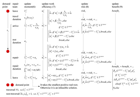
Figure 1.
Work flow of a repair team.
Equation (1) represents maximizing the total repair benefits of all repair teams. Equation (2) represents minimizing the total risks. Constraint (3) represents the importance degree of the demand points with the time window penalty. Constraint (4) represents the fact that each demand point is served by, at most, one repair team. Constraint (5) represents the fact that the number of vehicles entering the demand point is equal to the number of times the demand point is served. Figure 1 shows the workflow of a repair team leaving the previous demand point for the next demand point, starting repairing after rest, and leaving the next demand point after repair. Constraint (6) represents the updates of the moment. Constraint (7) represents the updates of the repair team’s work efficiency. The current work efficiency is not higher than the optimal work efficiency for at all times. Constraint (8) represents the updates of risks taken by the repair team before the deadline . Constraint (9) represents the updates of benefits created by the repair team after completion of each repair task.
5. Methods
The following can be seen from the above analysis:
- (1)
- The task scheduling of circuit repair is an extension of VRP [36], which is also NP-hard. Traditional algorithms (branch bound, dynamic programming, etc.) cannot solve the “combinatorial explosion” problem in a short time [37].
- (2)
- Once the order of the demand points, the repair status, and the tasks allocation are provided, by optimizing the rest duration there is at least one local optimal solution with high-benefits or low-risks. However, it is difficult to use traditional algorithms to solve the optimization problem of multimodal functions [38].
- (3)
- Traditional optimization algorithms often use weighted methods to convert multi-objective problems into single-objective problems [39], or use fuzzy optimization to solve them [40]. However, these algorithms have problems, such as difficulty in determining parameters, and cannot effectively solve multi-objective problems.
Therefore, in this article, we adopted multi-objective intelligent optimization algorithms to solve the task scheduling of circuit repair. The model in this article has many constraints and the coding method is complex. The algorithms in literature [25,26,27,28,29,30] are not convenient to solve the problem proposed in this article. However, the multi-objective genetic algorithm NSGA-II [4] is one of the best and most widely used algorithms at present in solving multi-objective optimization problems [2]. The multi-objective genetic algorithms, SPEA2 [5] and MOEA/D [6], are classics and widely used in the engineering field. These three algorithms have good reliability, robustness and scalability. Therefore, we performed multi-layer coding, and discrete and continuous hybrid coding on the basis of these three algorithms to solve more complex problems.
The three algorithms have strong global search abilities, but weak local search abilities, are slow to converge and prone to early maturity. The local search algorithm, 2-Opt [3] is often combined with other algorithms to improve the local search ability and speed up the convergence speed. The Differential Evolution (DE) algorithm [41] has high reliability and fast convergence speed. Therefore, the 2-Opt algorithm was used to optimize the repair order, and the DE algorithm was used to optimize the rest duration, in order to improve the local solution accuracy and speed up the convergence of the three algorithms above. We attempted to find a suitable combination of algorithms to effectively solve the new problems proposed in this article, without focusing too much on the innovation of operators in hybrid algorithms.
5.1. Encoding and Decoding
5.1.1. Encoding
Considering factors such as multiple repair teams repairing multiple demand points to a certain status in a certain order, and the uncertainty of the rest duration before repairs, this article designed four-layer coding to solve the problem. The first layer of integer coding represents the order of repair demand points. The second layer of integer coding indicates that each demand point is repaired to a certain status. The third layer of continuous coding indicates the rest duration after the repair teams arrive at the demand points. The fourth layer of integer coding indicates the grouping positions of repair teams.
5.1.2. Decoding
As shown in Figure 2, repair team 1 starts repairing from the 1st demand point to the 5 − 1th demand point (fourth layer coding). It repairs demand points 7∼3∼8∼5 (first layer coding), in turn, to the status 1∼3∼4∼3 (second layer coding). It rests for 0.0∼8.4∼12.1∼6.3 min (third layer coding) before repairing the demand points. Repair team 2 starts repairing from the 5th demand point to the 8 − 1th demand point (fourth layer coding). It repairs demand points 2∼1∼4 (first layer coding), in turn, to the status 1∼5∼2 (second layer coding). It rests for 9.8∼20.1∼0.0 min (third layer coding) before repairing the demand points. Repair team 3 starts repairing from the 8th demand point to the (10+1)-1th demand point (fourth layer coding). It repairs demand points 9∼6∼10 (first layer coding), in turn, to the status 3∼3∼1(second layer coding). It rests for 14.5∼22.9∼0.0 min (third layer coding) before repairing the demand points. Due to the deadline, the repair tasks of all demand points may not be completed.
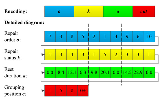
Figure 2.
Encoding and decoding diagram.
5.2. Operator Design
5.2.1. Genetic Algorithm (GA)
1. Selection: Use a binary tournament strategy to select better individuals in the population for getting the mating Pool.
Explanation: It is easy to operate and avoids falling into a local optimal solution.
2. Crossover:
(1) Cross repair order: According to the crossover probability Pc, randomly exchange a certain piece of the code in the two chromosomes. After exchanging each point, process repeated code in each chromosome. Perform corresponding operations on the corresponding points of the repair status and rest duration code.
Explanation: The repairable status and workload of each demand point are inconsistent, so the repair status and rest duration should be operated accordingly.
(2) Cross rest duration: According to the crossover probability Pc, randomly select the point i to perform random weight = rand crossover on the two chromosomes ChromA and ChromB:
Explanation: This improves global search capabilities of GA and also avoids frequent handling of out-of-bounds for repair teams’ maximum rest duration caused by crossover.
Note: Only here the meaning of the symbols A, B, i are inconsistent with the above.
3. Mutation:
(1) Mutate repair order: According to the mutation probability Pm, randomly select two points in a chromosome for exchange. Perform corresponding operations on the corresponding points of the repair status and rest duration code.
Explanation: The repairable status and workload of each demand point are inconsistent, so the repair status and rest duration should be operated accordingly.
(2) Mutate repair status: According to the mutation probability Pm, randomly select the repairable status for mutation point by point.
Explanation: The repairable status of each demand point is inconsistent. The crossover inevitably produces a large number of invalid solutions. For convenience, only mutation is considered.
(3) Mutate rest duration: According to the mutation probability Pm, randomly select the values in (0, max_t) for mutation point by point.
Explanation: Mutating with the values in (0, max_t) avoids frequent handling of out-of-bounds for repair teams’ maximum rest duration caused by mutation.
(4) Mutate grouping position: According to the mutation probability Pm, randomly select m−1 integers in the interval [2, n] and sort them from small to large for mutation on the entire code of the grouping position.
Explanation: The crossover of the grouping position code inevitably destroys the order of the grouping position from small to large, or generates repeated grouping positions. This produces an invalid solution. Therefore, for convenience, only use the mutation on the entire code of the grouping position.
The processes of GA1 and GA2 are shown in Operators 1.1 and 1.2.
| Operator 1.1: GA1 | |
| INPUT: | Parent with the size of pop_Parent |
| OUTPUT: | Son with the size of pop_Parent |
| Step 1: | Get a mating Pool with the size of pop_Pool from the Parent by Selection. |
| Step 2: | Randomly select two chromosomes from the Pool to cross repair order, mutate repair status, cross rest duration, and mutate grouping position. If a feasible solution is generated, add it to the Son_c population until its size is Pc × pop_Parent. |
| Step 3: | Randomly select a chromosome from the Pool to mutate repair order, mutate repair status, mutate rest duration, and mutate grouping position. If a feasible solution is generated, add it to the Son_m population until its size is Pm × pop_Parent. |
| Step 4: | Combine the Son_c and Son_m to get Son = [Son_c; Son_m]. |
| Operator 1.2: GA2 | |
| INPUT: | Parent with the size of 2 |
| OUTPUT: | Son with the size of 2 |
| Ifrand<Pc | Select these two chromosomes from the Parent to cross repair order, mutate repair status, cross rest duration, and mutate grouping position. If a feasible solution is generated, add it to the Son population until its size is 2. |
| Else | Randomly select a chromosome from the Parent to mutate repair order, mutate repair status, mutate rest duration, and mutate grouping position. If a feasible solution is generated, add it to the Son population until its size is 2. |
5.2.2. The 2-Optimization Algorithm (2-Opt)
In terms of code, the 2-Opt, and its derivatives, exhibit reversals of a piece of code. This article proposes the following operators for task scheduling of circuit repair.
1. Reversal-1: Randomly select a piece of code from the chromosome repair order code for reversal. Perform the corresponding operation on the corresponding points of the repair status and rest duration code.
2. Reversal-2: Randomly select a piece of code from the chromosome repair order code for reversal. Perform the corresponding operation on the corresponding points of the repair status code.
Explanation: Since the rest duration is affected by the work efficiency of repair teams, the professional coefficients of the repair teams and the risk factors of demand points, two reversal operators are used to generate two new individuals.
The process of 2-Opt is shown in Operator 2.
| Operator 2: 2-Opt | |
| INPUT: | Son with the size of pop_Son |
| OUTPUT: | Son with the size of pop_Son |
| For each individual in the population, perform 2-Opt by Reversal-1 and Reversal-2 respectively to generate two new individuals. If there is a feasible solution in the new individuals and it dominates the original individual, the original individual is replaced by the best. | |
5.2.3. Differential Evolution Algorithm (DE)
1. Initialization: Use the population truncation strategy in the multi-objective optimization algorithms to select a sub-population and optimize the rest duration code. MOEA/D has no population truncation strategy and so it prefers non-dominant individuals. In order to respect the purpose of MOEA/D to pursue a uniform distribution of the solution set, the dominant individuals are randomly selected to fill the sub-population until its size is pop_DE.)
Explanation: In order to reduce the amount of computation, only perform DE on the better sub-population in the population.
2. Mutation and Crossover: Use the mutation and crossover of DE/rand/1/bin.
Explanation: The “rand” is adopted instead of the “best” because the rest duration is affected by factors such as the work efficiency of the repair teams and the risk factors of demand points.
3. Boundary processing: If the rest duration is greater than , it will be replaced by a random value in .
Explanation: It improves the local search ability of DE and ensures that new individuals generated are feasible solutions.
4. Selection operator: If the new individual is a feasible solution and dominates the original individual, the original individual is replaced.
Explanation: The idea of the greedy algorithm drives the algorithm to choose a better solution.
The process of DE is shown in Operator 3.
| Operator 3: DE | |
| INPUT: | Parent with the size of pop_Parent |
| OUTPUT: | Parent with the size of pop_Parent |
| Step 1: | Select a f1 sub-population with the size of pop_DE from the Parent by the Initialization. |
| Step 2: | Perform Crossover, Mutation and Boundary processing in the rest duration coding part of f1 to generate a new f2 sub-population. |
| Step 3: | If an individual in f2 is feasible and dominates the corresponding individual in f1, replace it in f1 with it in f2. |
| Step 4: | If the iteration termination condition is satisfied, output the new Parent. Otherwise go to Step 2 to continue the iteration. |
5.3. Algorithms Process
We did not repeat the NSGA-II [4], SPEA2 [5], MOEA/D [6] algorithms process, population update and other strategies, but directly enumerated the processes of the hybrid algorithms NSGAII-2Opt-DE(N2D), SPEA2-2Opt-DE(S2D) and MOEA/D-2Opt-DE(M2D) as Algorithms 1, 2 and 3.
| Algorithm 1: N2D | |
| INPUT: | pop_GA, termination condition |
| OUTPUT: | Approximate Pareto optimal solution set |
| Step 1: | Initialization parameters. |
| Step 2: | Randomly generate a feasible solution set with the size of pop_GA to get Parent. Calculate the objective function value. Perform fast-non-dominated-sort and crowding-distance-assignment. |
| Step 3: | Generate Son = GA1(Parent) with the size of pop_GA by GA1. Calculate the objective function value. |
| Step 4: | Update Son = 2-Opt(Son) by 2-Opt. Calculate the objective function value. |
| Step 5: | Combine Parent and Son to get Combine = [Parent; Son]. Perform fast-non-dominated-sort and crowding-distance-assignment. |
| Step 6: | Select a new Parent with the size of pop_GA from Combine by the elite strategy. Perform fast-non-dominated-sort and crowding-distance-assignment. |
| Step 7: | Determine whether to perform DE. If so, Parent = DE(Parent). Perform fast-non-dominated-sort and crowding-distance-assignment. Otherwise, go to Step 8. |
| Step 8: | If the termination condition is satisfied, output the non-dominated solution set in Parent. Otherwise, go to Step 3 to continue the iteration. |
| Algorithm 2: S2D (In this article, Parent corresponds to in the original algorithm. Son corresponds to in the original algorithm.) | |
| INPUT: | pop_GA, termination condition |
| OUTPUT: | Approximate Pareto optimal solution set |
| Step 1: | Initialization parameters. |
| Step 2: | Randomly generate a feasible solution set with the size of pop_GA to get Parent. Calculate the objective function value. Calculate the fitness function. |
| Step 3: | Generate Son = GA1(Parent) with the size of pop_GA by GA1. Calculate the objective function value. |
| Step 4: | Update Son = 2-Opt(Son) by 2-Opt. Calculate the objective function value. |
| Step 5: | Combine Parent and Son to get Combine = [Parent; Son]. Calculate the fitness function. |
| Step 6: | Select a new Parent with the size of pop_GA from Combine by the environmental selection. Calculate the fitness function. |
| Step 7: | Determine whether to perform DE. If so, Parent = DE(Parent). Calculate the fitness function. Otherwise, go to Step 8. |
| Step 8: | If the termination condition is satisfied, output the non-dominated solution set in Parent. Otherwise, go to Step 3 to continue the iteration. |
| Algorithm 3: M2D (Archive corresponds to EP in the original algorithm. 1_Son corresponds to y′ in the original algorithm.) | |
| INPUT: | pop_GA, termination condition |
| OUTPUT: | Approximate Pareto optimal solution set |
| Step 1: | Initialization parameters. For each individual, randomly generate weights and find neighbors with the size of pop_Neighbor according to Euclidean distance. |
| Step 2: | Randomly generate a feasible solution set with the size of pop_GA to get Parent. Calculate the objective function value. Find the maximum value of each objective function value to get vector z. |
| Step 3: | Store non-dominated individuals in Parent to get Archive. |
| Step 4: | Perform the following for each individual in Parent: Randomly select two neighbors to get Neighbor = [Neighbor1; Neighbor2]. Generate Son = GA2(Neighbor) with the size of 2 by GA2. Update Son = 2-Opt(Son) by 2-Opt. Calculate the objective function value. Select a non-dominated individual 1_Son in Son. Update z. Calculate and update neighbors. |
| Step 5: | Determine whether to perform DE. If so, Parent = DE(Parent). Update z. Otherwise, go to Step 6. |
| Step 6: | Select the non-dominated individual Nd from Parent. Combine Nd and the original Archive to get Combine = [Archive; Nd]. |
| Step 7: | Select the non-dominated individuals from the Combine to get the Archive. If its size pop_Archive > pop_GA, some individuals will be randomly discarded to make pop_Archive = pop_GA. |
| Step 8: | If the termination condition is satisfied, output the Archive. Otherwise, go to Step 4 to continue the iteration. |
5.4. Algorithm Scientificity
The Schema Theorem [42] points out that, under selection, crossover and mutation of GA, low-level, short-range, and high-fitness patterns grow exponentially in the population. Fogel [43] proved that the algorithms converged with probability 1 when the evolutionary sequence of individuals in the population being monotonic was satisfied. Rudolph [44] proved that the multi-objective evolutionary algorithms converged with probability 1 when monotonic screening was based on Pareto ranking.
In this article, the NSGAII, SPEA2 algorithms adopted the elite strategy [45] to update the population. The MOEAD algorithm was based on the monotonic optimization of “”. In the hybrid algorithms, 2-Opt and DE were also updated through greedy thinking, according to the Pareto dominance relationship, so the scientificity of the algorithms was guaranteed.
6. Evaluation Indicators
6.1. Algorithms’ Solution Quality
The task scheduling of circuit repair has the following characteristics:
- (1)
- It is NP-hard. The intelligent optimization algorithms used involve continuous coding. so even a larger population and more iterations could only obtain an approximate Pareto optimal solution set.
- (2)
- It is a multi-objective optimization problem, involving preference, and is dynamic and multimodal at the same time.
According to the above characteristics, this article analyzed the indicators in the literature [30,31,32], and selected the following commonly used indicators to evaluate the algorithms:
- (1)
- C-metric (C) [7] was used to evaluate the convergence of the sets solved by the algorithms;
- (2)
- Spacing(S) [8] was used to evaluate the distribution of the sets solved by the algorithms;
- (3)
- [9] was used to evaluate the spread of the sets solved by the algorithms.
6.2. Algorithms’ Solution Efficiency
This article designed a comprehensive evaluation indicator area. For convenience, this indicator is illustrated using the problem in this article as an example.
Definition:
We established a Cartesian coordinate system with benefit as the horizontal axis and risk as the vertical axis. We added the origin (0, 0) to the approximate Pareto optimal solution set solved by an algorithm, and drew the solution set in the coordinate system. We connected adjacent points to form a polyline. On the vertical axis, we selected the upper bound “md” of risk and drew a straight line parallel to the horizontal axis. The area above the polyline and below the straight line was denoted as area.
Supplement:
- (1)
- The benefit and risk are not less than 0, and the point (0, 0) must belong to the true Pareto optimal solution set. Therefore, this point was selected as a reference point to be added to the approximate Pareto optimal solution set.
- (2)
- The work efficiency of m repair teams is not greater than . The risk factors of routes or demand points are not greater than 1. The deadline for circuit repair is . Therefore, was selected as the upper bound of risk.
- (3)
- This area was used to evaluate the 2-objective optimization algorithm. If the area was generalized to a hypervolume, it could be used to evaluate multi-objective optimization algorithms.
Properties: From the analysis in 5.4, it could be seen that the approximate Pareto optimal solution set converged to the real Pareto optimal solution set. Therefore, the area also converged. From the definition, the following properties were clearly established:
- (1)
- The faster the area changed with the number of iterations, the faster the algorithm converged;
- (2)
- The larger the area was, the closer the approximate Pareto optimal surface was to the real Pareto optimal surface, and the better the quality of the solution set was;
- (3)
- The larger the area was, the better the spread of the solution set on the other side of the reference point (0, 0) was;
- (4)
- We drew a curve, which was generated by the area changing with the number of iterations. The smaller the number and degree of curve mutation, the denser the distribution of the solution set in the approximate Pareto optimal surface was. Figure 3 shows why the smoothness of the curve was destroyed.
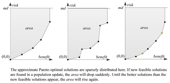 Figure 3. Diagram of the causes of area mutation.
7. Computational Experiments
In this part, computational experiments were carried out to illustrate the scientificity of the strategies, model, algorithms and evaluation indicator proposed in this article. The proposal was implemented using Matlab2018a, and the experiments were run on a desktop computer with a Processor Intel(R) Core(TM) i5-9400F CPU @2.9GHz, 16GB of RAM, and running Microsoft Windows 7 Pro 64 bits system.
7.1. Parameter Settings
The algorithms’ parameters were set as follows:
- (1)
- GA: The number of iterations was 600, the population size was 200, the mating pool size was 100, the crossover probability was 0.9, the mutation probability was 0.1, and the number of neighbors was 20.
- (2)
- DE: The number of iterations was 10, the population size was 100, the mutation operator was 0.5, and the crossover operator was 0.1.
The problem parameters were set as follows:
- (1)
- The initial positions of the repair teams and the demand points, the upper limits of the time windows, and the importance degree penalty coefficients were taken from the literature [2]. We assumed that all faults had occurred, that is, the lower limits of the time windows were 0. The deadline was pointed out by the decision makers. In order to reflect the lack of time, this article took the deadline to be equal to 410 min, which was less than the upper limit of the time windows of 5 demand points in the 20 demand points.
- (2)
- According to the model in this article, the other information in the literature [2] was transformed and adjusted as shown Table 2 and Table 3.
Table 2. Demand points information.
Table 3. Demand points information.
We did not have the ability to obtain comprehensive data. Therefore, we randomly generated 10 data sets according to a uniform distribution, which allowed us to study various cases with equal probability. The data included the risk factors and the professional coefficients . Then, we used the algorithms mentioned in Section 5.3 to conduct computational experiments, and used the indicators mentioned in Section 6 for evaluation. The obtained data is shown in Table 4, Table 5, Table 6 and Table 7 and Figure 4, Figure 5 and Figure 6.
Table 4.
The calculation results of C.
Table 5.
The calculation results of S (Order of magnitude ).
Table 6.
The calculation results of (Order of magnitude ).
Table 7.
The calculation results of area (Order of magnitude ).
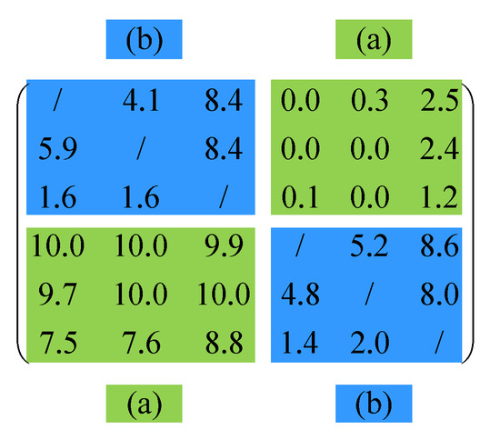
Figure 4.
The mean of the data in Table 4.
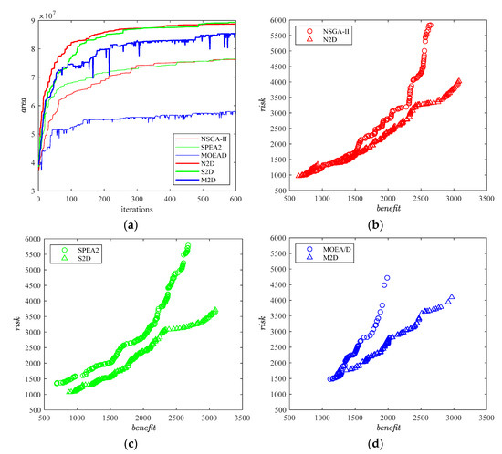
Figure 5.
A simulation of case 1 as an example to show the convergence speed of the algorithms and the distribution of the solution sets (Task scheduling information and initial population settings were consistent). (a) The convergence speed of the algorithms; (b) The distribution of the sets solved by NSGA-II and N2D; (c) The distribution of the sets solved by SPEA2 and S2D; (d) The distribution of the sets solved by MOEA/D and M2D.
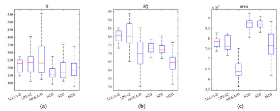
Figure 6.
Case 1 as an example to show the boxplots on the indicators of the algorithms. (a) The boxplots on S; (b) The boxplots on ; (c) The boxplots on area.
7.2. Experimental Results and Analysis
In this article, 1000 experiments were conducted. The comparison of the 6 algorithms on the indicator C is shown in Table 4 and Figure 4. The means on the indicators, including S, and area, are shown in Table 5, Table 6 and Table 7. The boxplots are shown in Figure 6.
The algorithms’ convergence can be seen from Table 4 and Figure 4. Figure 4 is the average of C for the 10 cases in Table 4.
The 2-Opt and DE significantly improved the convergence of the hybrid algorithms. In addition, NSGA-II performed fast non-dominated sort and crowding-distance-assignment, and SPEA2 calculated the fitness function. When there were few non-dominated solutions, the sub-optimal solutions had the opportunity to be optimized into non-dominated solutions by 2-Opt and DE. However, MOEA/D only stored the non-dominated solutions of each generation. When there were few non-dominated solutions, other dominated individuals could be randomly selected for 2-Opt and DE optimization. The randomness was large, which affected the convergence of MOEA/D.
The distribution of the sets solved by the algorithms can be seen in Table 5.
- (1)
- NSGA-II was better than SPEA2 by 70%, SPEA2 was better than MOEA/D by 70%, and MOEA/D was better than NSGA-II by 10%.
- (2)
- N2D was better than S2D by 70%, S2D was better than M2D by 80%, and M2D was better than N2D by 10%.
- (3)
- N2D was better than NSGA-II by 80%, S2D was better than SPEA2 by 60%, and M2D was better than MOEA/D by 60%.
The spread of the sets solved by the algorithms can be seen in Table 6.
- (1)
- NSGA-II was better than SPEA2 by 80%, SPEA2 was better than MOEA/D by 100%, and MOEA/D was better than NSGA-II by 0%.
- (2)
- N2D was better than S2D by 60%, S2D was better than M2D by 100%, and M2D was better than N2D by 0%.
- (3)
- N2D was better than NSGA-II by 0%, S2D was better than SPEA2 by 0%, M2D was better than MOEA/D by 10%.
NSGA-II performed crowding-distance-assignment, SPEA2 adopted a density information, which resulted in better distribution and spread. However, the MOEA/D algorithm pursued a uniform distribution of solutions, and had no tendency to retain extreme solutions, so the spread was poorer. In addition, the hybrid algorithms reduced the risks more than the original algorithms under the same benefits. Therefore, the spread of the hybrid algorithms was poorer.
From Table 7, we can see the comprehensive performance of the algorithms, which includes the convergence of algorithms and the one-sided spread of the solution set away from the origin (0, 0).
- (1)
- NSGA-II was better than SPEA2 by 50%, SPEA2 was better than MOEA/D by 100%, and MOEA/D was better than NSGA-II by 0%.
- (2)
- N2D was better than S2D by 30%, S2D was better than M2D by 100%, and M2D was better than N2D by 0%.
- (3)
- N2D was better than NSGA-II by 100%, S2D was better than SPEA2 by 100%, M2D was better than MOEA/D by 100%.
The solution sets of the hybrid algorithms had better convergence, and the area was larger.
The convergence speed of the algorithms and the distribution of the solution sets can be seen from Figure 5.
- (1)
- The convergence speed of the algorithms can be seen from Figure 5a. NSGA-II was not much different from SPEA2, but both were better than MOEA/D. N2D was not much different from S2D, but both were better than M2D.
- (2)
- The distribution of the solution sets can be seen from Figure 5b–d. NSGA-II was not much different from SPEA2, but both were better than MOEA/D. N2D was not much different from S2D, but both were better than M2D. N2D, S2D and M2D were better than NSGA-II, SPEA2 and MOEA/D.
The distribution and stability of the algorithms on the indicators, including S, and area, can be seen from Figure 6.
- (1)
- Overall, the stability of NSGA-II, SPEA2 and MOEA/D on these indicators decreased, in turn. The stability of N2D, S2D and M2D on the indicators decreased, in turn.
- (2)
- The stabilities of N2D, S2D and M2D on the indicators were not worse than those of NSGA-II, SPEA2 and MOEA/D, respectively.
To sum up, NSGA-II and N2D were more stable in terms of convergence, distribution and spread, while MOEA/D and M2D were less stable. According to the data in Table 4, Table 5, Table 6 and Table 7 and the Figure 4, Figure 5 and Figure 6, it can be seen that the area designed in this article was reasonable.
8. Conclusions and Outlook
The original support mode of circuit repair is no longer applicable. Therefore, we focused on improving the support mode of circuit repair. First, we proposed three rest strategies, and considered the scheduling optimization of flexible rest for the repair teams. We built a mathematical model, which aimed to maximize benefits and minimize risks with constraints such as geographic information and resource, etc. Second, we designed three hybrid algorithms, namely, N2D, S2D and M2D. The algorithms had good solution qualities and convergence speeds. Third, we designed a comprehensive evaluation indicator, area, which could evaluate the convergence speed of the multi-objective optimization algorithms. Finally, we conducted computational experiments to verify the scientificity of the rest strategies, model, algorithms and evaluation indicator proposed in this article.
Since the real data collection and the evaluation were not comprehensive enough, the following aspects could be studied in the future:
- (1)
- Various repair teams have different personnel and equipment. There may be differences in the reliability of repairing a certain demand point to the same status. This data could be collected, evaluated, and incorporated into existing literature models and algorithms.
- (2)
- The current parameters are single. Different time windows for various repair statuses, different penalty coefficients for the importance degrees of various demand points, different routes selection or inconsistent detour coefficients, due to different thrust-to-weight ratios of heterogeneous vehicles, and different detour coefficients of asymmetric routes could be collected and evaluated. These data could be integrated into existing literature models and algorithms.
Author Contributions
Conceptualization, S.L. and X.Q.; methodology, S.L. and L.L.; software, S.L.; validation, S.L., X.Q. and L.L.; formal analysis, S.L.; investigation, S.L.; resources, X.Q.; data curation, S.L.; writing—original draft preparation, S.L.; writing—review and editing, X.Q.; visualization, S.L.; supervision, X.Q.; project administration, X.Q.; funding acquisition, X.Q. All authors have read and agreed to the published version of the manuscript.
Funding
This research was funded by the National Natural Science Foundation of China, grant number 61877067” and the “Foundation of Equipment research, grant number 80904010301”.
Institutional Review Board Statement
Not applicable.
Informed Consent Statement
Not applicable.
Data Availability Statement
Part of the data generated during this study is included in the published article [2]. Due to incomplete data in article [2], part of the data was randomly generated by the authors of this article. All the data generated and analyzed during the current study is available from the corresponding author on reasonable request.
Acknowledgments
We thank the editors and reviewers for their guidance and assistance. In addition, we acknowledge the support of the foundation, including the National Natural Science Foundation of China (Grant No. 61877067), and the Foundation of Equipment research (Grant No. 80904010301).
Conflicts of Interest
The authors declare no conflict of interest.
References
- Liu, Y.; Chen, C.L.; Zan, X.; Chen, W.L.; Zhang, L.J. Multi-objective dynamic scheduling with accompanying repair tasks under complex constraints. Acta Armamentarii 2019, 40, 621–628. [Google Scholar]
- Liu, Y.; Jia, J.; Zhang, Z.Q.; Jin, F. Multi-objective dynamic scheduling of circuit repair based on improved NSGA-II. Conf. Ser. Mater. Sci. Eng. 2021, 1043, 022011. [Google Scholar] [CrossRef]
- Zhang, J. An Improved Genetic Algorithm with 2-Opt Local Search for the Traveling Salesman Problem. International Conference on Application of Intelligent Systems in Multi-Modal Information Analytics; Springer: Cham, Switzerland, 2021; pp. 404–409. [Google Scholar]
- Verma, S.; Pant, M.; Snasel, V. A comprehensive review on NSGA-II for multi-objective combinatorial optimization problems. IEEE Access 2021, 9, 57757–57797. [Google Scholar] [CrossRef]
- Quenum, J.G. Distributed Optimisation of Perfect Preventive Maintenance and Component Replacement Schedules Using SPEA2. In Intelligent Computing and Optimization, Proceedings of the 3rd International Conference on Intelligent Computing and Optimization 2020 (ICO 2020); Springer Nature: Berlin, Germany, 2021; Volume 1324, p. 297. [Google Scholar]
- Pang, L.M.; Ishibuchi, H.; Shang, K. Using a Genetic Algorithm-Based Hyper-Heuristic to Tune MOEA/D for a Set of Various Test Problems. In IEEE Congress on Evolutionary Computation (CEC); IEEE: Piscataway, NJ, USA, 2021; pp. 1486–1494. [Google Scholar]
- Huang, Y.Y.; Pan, Q.K.; Gao, L.; Miao, Z.H.; Peng, C. A two-phase evolutionary algorithm for multi-objective distributed assembly permutation flowshop scheduling problem. Swarm Evol. Comput. 2022, 74, 101128. [Google Scholar] [CrossRef]
- Chiu, C.C.; Lai, C.M. Multi-objective missile boat scheduling problem using an integrated approach of NSGA-II, MOEAD, and data envelopment analysis. Appl. Soft Comput. 2022, 127, 109353. [Google Scholar] [CrossRef]
- Zitzler, E.; Deb, K.; Thiele, L. Comparison of multi-objective evolutionary algorithms: Empirical results. Evol. Comput. 2000, 8, 173–195. [Google Scholar] [CrossRef]
- Wen, X.Y.; Lian, X.N.; Qian, Y.J.; Zhang, Y.Y.; Wang, H.Q.; Li, H. Dynamic scheduling method for integrated process planning and scheduling problem with machine fault. Robot. Comput.-Integr. Manuf. 2022, 77, 102334. [Google Scholar] [CrossRef]
- Dong, C.; Zhou, L. Optimization Algorithm for Freight Car Transportation Scheduling Optimization Based on Process Scheduling Optimization. In Cloud Computing and Security; Springer: Cham, Switzerland, 2018; pp. 528–538. [Google Scholar]
- Tian, Y.; Xiong, T.F.; Liu, Z.Y.; Mei, Y.; Wan, L. Multi-objective multi-skill resource-constrained project scheduling problem with skill switches: Model and evolutionary approaches. Comput. Ind. Eng. 2022, 167, 107897. [Google Scholar] [CrossRef]
- Zhu, L.; Lin, J.; Li, Y.Y.; Wang, Z.J. A decomposition-based multi-objective genetic programming hyper-heuristic approach for the multi-skill resource constrained project scheduling problem. Knowl.-Based Syst. 2021, 225, 107099. [Google Scholar] [CrossRef]
- An, Y.J.; Chen, X.H.; Li, Y.H.; Zhang, J.; Jiang, J.W. Flexible job-shop scheduling and heterogeneous repairman assignment with maintenance time window and employee timetable constraints. Expert Syst. Appl. 2021, 186, 115693. [Google Scholar] [CrossRef]
- Gong, G.L.; Deng, Q.W.; Gong, X.R.; Huang, D. A non-dominated ensemble fitness ranking algorithm for multi-objective flexible job-shop scheduling problem considering worker flexibility and green factors. Knowl.-Based Syst. 2021, 231, 107430. [Google Scholar] [CrossRef]
- de Oliveira, S.M.; Bezerra, L.C.T.; Stützle, T.; Dorigo, M.; Wanner, E.F.; de Souza, S.R. A computational study on ant colony optimization for the traveling salesman problem with dynamic demands. Comput. Oper. Res. 2021, 135, 105359. [Google Scholar] [CrossRef]
- He, P.F.; Hao, J.K. Hybrid search with neighborhood reduction for the multiple traveling salesman problem. Comput. Oper. Res. 2022, 142, 105726. [Google Scholar] [CrossRef]
- Altabeeb, A.M.; Mohsen, A.M.; Abualigah, L.; Ghallab, A. Solving capacitated vehicle routing problem using cooperative firefly algorithm. Appl. Soft Comput. 2021, 108, 107403. [Google Scholar] [CrossRef]
- Pan, B.B.; Zhang, Z.Z.; Lim, A. Multi-trip time-dependent vehicle routing problem with time windows. Eur. J. Oper. Res. 2021, 291, 218–231. [Google Scholar] [CrossRef]
- Vincent, F.T.; Jewpanya, P.; Perwira Redi, A.A.N.; Tsao, Y.C. Adaptive neighborhood simulated annealing for the heterogeneous fleet vehicle routing problem with multiple cross-docks. Comput. Oper. Res. 2021, 129, 105205. [Google Scholar]
- Pan, W.X.; Liu, S.Q. Deep reinforcement learning for the dynamic and uncertain vehicle routing problem. Appl. Intell. 2022, 1–18. [Google Scholar] [CrossRef]
- Cai, J.Q.; Peng, Z.H.; Ding, S.X.; Sun, J.B. Problem-specific multi-objective invasive weed optimization algorithm for reconnaissance mission scheduling problem. Comput. Ind. Eng. 2021, 157, 107345. [Google Scholar] [CrossRef]
- Chen, L.Z.; Liu, W.L.; Zhong, J.H. An efficient multi-objective ant colony optimization for task allocation of heterogeneous unmanned aerial vehicles. J. Comput. Sci. 2022, 58, 101545. [Google Scholar] [CrossRef]
- Liu, Y.; Chen, C.L.; Chen, W.L.; Guo, Y.M. Multi-objective dynamic scheduling of fixed-point repairing tasks based on pareto improved VNS-MMAS. Syst. Eng. Electron. 2020, 42, 356–364. [Google Scholar]
- Zeedan, M.; Attiya, G.; EI-Fishawy, N. Enhanced hybrid multi-objective workflow scheduling approach based artificial bee colony in cloud computing. Computing 2022, 1–31. [Google Scholar] [CrossRef]
- Qin, S.; Pi, D.C.; Shao, Z.S.; Xu, Y. Hybrid collaborative multiobjective fruit fly optimization algorithm for scheduling workflow in cloud environment. Swarm Evol. Comput. 2022, 68, 101008. [Google Scholar] [CrossRef]
- Chen, R.H.; Yang, B.L.; Wang, S.; Cheng, Q.Q. An effective multipopulation grey wolf optimizer based on reinforcement learning for flow shop scheduling problem with multi-machine collaboration. Comput. Ind. Eng. 2021, 162, 107738. [Google Scholar] [CrossRef]
- Sanaj, M.S.; Joe Prathap, P.M. Nature inspired chaotic squirrel search algorithm (CSSA) for multi objective task scheduling in an iaas cloud computing atmosphere. Eng. Sci. Technol. Int. J. 2020, 23, 891–902. [Google Scholar] [CrossRef]
- Srichandan, S.; Kumar, T.A.; Bibhudatta, S. Task scheduling for cloud computing using multi-objective hybrid bacteria foraging algorithm. Future Comput. Inform. J. 2018, 3, 210–230. [Google Scholar] [CrossRef]
- Tan, W.H.; Yuan, X.F.; Huang, G.M.; Liu, Z.X. Low-carbon joint scheduling in flexible open-shop environment with constrained automatic guided vehicle by multi-objective particle swarm optimization. Appl. Soft Comput. 2021, 111, 107695. [Google Scholar] [CrossRef]
- Xu, X.; Xu, G.X.; Chen, J.W.; Liu, Z.; Chen, X.B.; Zhang, Y.; Fang, J.G.; Gao, Y.K. Multi-objective design optimization using hybrid search algorithms with interval uncertainty for thin-walled structures. Thin-Walled Struct. 2022, 175, 109218. [Google Scholar] [CrossRef]
- Zhang, W.Q.; Yang, D.J.; Zhang, G.H.; Gen, M. Hybrid multi-objective evolutionary algorithm with fast sampling strategy-based global search and route sequence difference-based local search for VRPTW. Expert Syst. Appl. 2020, 145, 113151. [Google Scholar] [CrossRef]
- Wang, Y.L.; Limmer, S.; Olhofer, M.; Emmerich, M.; Bäck, T. Automatic preference based multi-objective evolutionary algorithm on vehicle fleet maintenance scheduling optimization. Swarm Evol. Comput. 2021, 65, 100933. [Google Scholar] [CrossRef]
- Azzouz, R.; Bechikh, S.; Ben Said, L.; Bechikh, S.; Datta, R.; Gupta, A. (Eds.) Dynamic Multi-objective Optimization Using Evolutionary Algorithms: A Survey; Springer: Cham, Switzerland, 2017; pp. 31–70. [Google Scholar]
- Liang, J.; Guo, Q.Q.; Yue, C.T.; Qu, B.Y.; Yu, K.J. A self-organizing multi-objective particle swarm optimization algorithm for multimodal multi-objective problems. Int. Conf. Swarm Intell. 2018, Volume 10941, 550–560. [Google Scholar]
- de Jonge, D.; Bistaffa, F.; Levy, J. Multi-objective vehicle routing with automated negotiation. Appl. Intell. 2022, 52, 16916–16939. [Google Scholar] [CrossRef]
- Mor, B.; Shabtay, D.; Yedidsion, L. Heuristic algorithms for solving a set of NP-hard single-machine scheduling problems with resource-dependent processing times. Comput. Ind. Eng. 2021, 153, 107024. [Google Scholar] [CrossRef]
- Cuevas, E.; G’alvez, J.; Toski, M.; Avila, K. Evolutionary-mean shift algorithm for dynamic multimodal function optimization. Appl. Soft Comput. 2021, 113, 107880. [Google Scholar] [CrossRef]
- Kumar, R.; Singh, S.J.; Bilga, P.S.; Singh, J.; Singh, S.; Scutaru, M.L.; Pruncu, C.I. Revealing the benefits of entropy weights method for multi-objective optimization in machining operations: A critical review. J. Mater. Res. Technol. 2021, 10, 1471–1492. [Google Scholar] [CrossRef]
- Mirzaie, N.; Banihabib, M.E.; Randhir, T.O.; Shahdany, S.M.H. Fuzzy particle swarm optimization for conjunctive use of groundwater and reclaimed wastewater under uncertainty. Agric. Water Manag. 2021, 256, 107116. [Google Scholar] [CrossRef]
- He, L.J.; Cao, Y.L.; Li, W.F.; Cao, J.J.; Zhong, L.C. Optimization of energy-efficient open shop scheduling with an adaptive multi-objective differential evolution algorithm. Appl. Soft Comput. 2022, 118, 108459. [Google Scholar] [CrossRef]
- Yin, X.F.; Li, P.K. An exact schema theorem for adaptive genetic algorithm and its application to machine cell formation. Expert Syst. Appl. 2011, 38, 8538–8552. [Google Scholar] [CrossRef]
- Fogel, D.B. Evolutionary Algorithms in Theory and Practice; John Wiley Sons Inc.: New York, NY, USA, 1997. [Google Scholar]
- Rudolph, G. Evolutionary search for minimal elements in partially ordered finite sets. Int. Conf. Evol. Program. 1998, volume 1447, 345–353. [Google Scholar]
- Leno, I.J.; Sankar, S.S.; Ponnambalam, S.G. Mip model and elitist strategy hybrid ga-sa algorithm for layout design. J. Intell. Manuf. 2018, 29, 369–387. [Google Scholar] [CrossRef]

Publisher’s Note: MDPI stays neutral with regard to jurisdictional claims in published maps and institutional affiliations. |
© 2022 by the authors. Licensee MDPI, Basel, Switzerland. This article is an open access article distributed under the terms and conditions of the Creative Commons Attribution (CC BY) license (https://creativecommons.org/licenses/by/4.0/).