Representative Points Based on Power Exponential Kernel Discrepancy

Abstract

Representative points (rep-points) are a set of points that are optimally chosen for representing a big original data set or a target distribution in terms of a statistical criterion, such as mean square error and discrepancy. Most of the existing criteria can only assure the representing properties in the whole variable space. In this paper, a new kernel discrepancy, named power exponential kernel discrepancy (PEKD), is proposed to measure the representativeness of the point set with respect to the general multivariate distribution. Different from the commonly used criteria, PEKD can improve the projection properties of the point set, which is important in high-dimensional circumstances. Some theoretical results are presented for understanding the new discrepancy better and guiding the hyperparameter setting. An efficient algorithm for searching rep-points under the PEKD criterion is presented and its convergence has also been proven. Examples are given to illustrate its potential applications in the numerical integration, uncertainty propagation, and reduction of Markov Chain Monte Carlo chains.

1. Introduction

Rep-points, also called principal points [1] or support points [2], can be viewed as a data reduction method or statistical simulation technique, and it has been widely applied in many areas. In the very beginning, many authors studied how to find the optimal rep-points for representing the univariate or bivariate normal distribution [3,4]. Then Refs. [1,5] extended the rep-points for the elliptical distributions. [6,7] used the rep-points as the refined Monte Carlo technique for approximating the integration or expectation. More applications of rep-points can be found in the uncertainty quantification [2,8,9] and Bayesian analysis [10,11,12].

A lot of statistical criteria, such as the mean square error [1,6,13,14,15], discrepancy [16], divergence [17], and statistical potential [18,19], are proposed to measure the representativeness of the point set with respect to the target distribution. In this paper, we mainly discuss the kernel discrepancy, which is also known as the maximum mean discrepancy in deep learning [20] and transfer learning [21]. The property of kernel discrepancy is determined by the corresponding kernel function. Analytic expressions of kernel discrepancy are available for particular distributions and particular kernel functions; see [16,22,23]. For obtaining rep-points from more general distributions, Ref. [24] proposed the kernel herding method based on some common kernel functions, such as Gaussian and Laplacian kernels, and they generated rep-points one by one with the greedy stochastic optimization algorithm. The support points (SP) method proposed by [2] is another kind of rep-points based on the negative Euclidean distance kernel discrepancy.

Note that the kernels in kernel herding and support points methods are isotropic, which means all the variables are considered active and the effects of all orders are equally important. However, when the dimension of the problem is relatively high, the active variables are usually sparse in practice. More attention should be paid to the representativeness of the projection distribution of rep-points. Some generalized $L_2$ discrepancies proposed by [25,26] can assure the low-dimensional space-filling properties by directly summing all local projection discrepancies. These discrepancies have concise expressions by using separable kernels and binomial theorem, but they are limited to the uniform distribution on the hypercube. Ref. [27] presented the projected support points (PSP) method by constructing a sparsity-inducing kernel, which assumes a prior on the hyperparameters of Gaussian kernel. However, compared with the SP method, the algorithm for generating PSP is computationally expensive since it is based on the block Majorization-Minimization algorithm framework [28] and includes sampling steps for hyperparameters.

There is an urgent need for an effective kernel discrepancy that encourages the preservation of low-dimensional representativeness and can be efficiently constructed. In this paper, the new discrepancy is developed from the power exponential kernel function [16,29,30], so we call it PEKD. Different from the average kernels in generalized $L_2$ discrepancies and the PSP method, we make use of the $L_{\alpha }$ norm in the power exponential kernel to regulate the representativeness of rep-points in subspaces of different projection dimensions. The contribution of this work is threefold. First, some theoretical analyses about the effect of the hyperparameter $\alpha$ on the low-dimensional structure of rep-points are presented. In particular, we demonstrate that the rep-points under PEKD just form a Latin hypercube design for uniform distribution on the hypercube, given a suitable choice of hyperparameters. Second, we introduce the successive convex approximation algorithm framework [28] to construct an efficiently parallelized algorithm for generating rep-points under PEKD, and its convergence has also been proven. Third, we illustrate the effectiveness of the new method with simulation studies for numerical integration, uncertainty propagation problems, and a real-world problem for MCMC reduction.

This paper is organized as follows. Section 2 recalls kernel discrepancies in the existing reference related with rep-points and introduces the proposed PEKD. Section 3 constructs an algorithm to generate rep-points under PEKD. Section 4 demonstrates the effectiveness of the new method with several examples. Section 5 concludes with thoughts on further work. For brevity, all proofs are postponed to the Appendix A.

2. Power Exponential Kernel Discrepancy

In this section, we first briefly introduce the kernel discrepancy [25] and the existing kernel functions used to generate rep-points. Then, we propose PEKD and analyze its theoretical properties.

2.1. Kernel Discrepancy

Let $\mathcal{X}\subseteq {\mathbb{R}}^p$, the binary function $\gamma :\mathcal{X}\times \mathcal{X}\to \mathbb{R}$ is called a symmetric positive kernel [16] if it satisfies two properties: (i) symmetric, $\gamma (\mathbf{x},\mathbf{y})=\gamma (\mathbf{y},\mathbf{x}),\forall \mathbf{x},\mathbf{y}\in \mathcal{X}$, and (ii) nonnegative definite, ∀$c_1,\dots ,c_n\in \mathbb{R}$, ${\mathbf{x}}_1,\dots ,{\mathbf{x}}_n\in \mathcal{X}$, ${\sum }_{i=1}^n{\sum }_{j=1}^n{c}_i\gamma ({\mathbf{x}}_i,{\mathbf{x}}_j)c_j\ge 0.$

Definition 1.

Let F be a distribution function on $\mathcal{X}\subseteq {\mathbb{R}}^p$, and let $F_{\mathcal{P}}$ be the empirical distribution function of a point set $\mathcal{P}={\left\{{\mathbf{x}}_i\right\}}_{i=1}^n\subseteq \mathcal{X}$. For a symmetric positive definite kernel γ, the kernel discrepancy between F and $F_{\mathcal{P}}$ is defined as:

$$\begin{array}{cc}\hfill D_{\gamma }^2(F,F_{\mathcal{P}}):& ={\int }_{\mathcal{X}}{\int }_{\mathcal{X}}\gamma (\mathbf{x},\mathbf{y})\mathrm{d}[F-F_{\mathcal{P}}]\left(\mathbf{x}\right)\mathrm{d}[F-F_{\mathcal{P}}]\left(\mathbf{y}\right)\hfill \\ \hfill & ={\int }_{\mathcal{X}}{\int }_{\mathcal{X}}\gamma (\mathbf{x},\mathbf{y})\mathrm{d}F\left(\mathbf{x}\right)\mathrm{d}F\left(\mathbf{y}\right)-\frac{2}{n}\sum _{i=1}^n{\int }_{\mathcal{X}}\gamma ({\mathbf{x}}_i,\mathbf{y})\mathrm{d}F\left(\mathbf{y}\right)+\frac{1}{n^2}\sum _{i,j=1}^n\gamma ({\mathbf{x}}_i,{\mathbf{x}}_j).\hfill \end{array}$$

(1)

Further, ${\mathcal{P}}^{*}={\left\{{\mathbf{x}}_i^{*}\right\}}_{i=1}^n$ is called the rep-points [22] of distribution F, if

$$D_{\gamma }^2(F,F_{{\mathcal{P}}^{*}})=\underset{\mathcal{P}\subseteq \mathcal{X}}{\min }{D}_{\gamma }^2(F,F_{\mathcal{P}}).$$

(2)

Lemma 1

(Koksma-Hlawka inequality; [25]). Let γ be a symmetric positive definite kernel on $\mathcal{X}$, and ${\mathcal{H}}_{\gamma }$ be the reproducing kernel Hilbert space for the kernel γ. F and $F_{\mathcal{P}}$ are as defined in Definition 1. The integration error of $g\in {\mathcal{H}}_{\gamma }$, defined as:

$$I(g;F,F_{\mathcal{P}}):=\left|{\int }_{\mathcal{X}}g\left(\mathbf{x}\right)dF\left(\mathbf{x}\right)-\frac{1}{n}\sum _{i=1}^{n}g\left({\mathbf{x}}_i\right)\right|,$$

(3)

can be uniformly bounded as:

$$I(g;F,F_{\mathcal{P}})\le {\parallel g\parallel }_{{\mathcal{H}}_{\gamma }}{D}_{\gamma }(F,F_{\mathcal{P}}).$$

(4)

2.2. Kernels in Existing Rep-Points Methods

2.2.1. Isotropic Kernel

Definition 2.

A kernel function γ is isotropic kernel, if it can be expressed as a function of the Euclidean distance between points, i.e., $\gamma (\mathbf{x},\mathbf{y})=h(\parallel \mathbf{x}-\mathbf{y}{\parallel }_2)$, where ${\parallel ·\parallel }_2$ is the Euclidean norm.

Gaussian kernel and Laplacian kernel, ${\gamma }_G(\mathbf{x},\mathbf{y})={exp\{-\theta \parallel \mathbf{x}-\mathbf{y}\parallel }_2^2\}$ and ${\gamma }_L(\mathbf{x},\mathbf{y})={exp\{-\theta \parallel \mathbf{x}-\mathbf{y}\parallel }_2\}$, are two well-known isotropic kernels, which are widely used in nonlinear classification and regression problems. Based on these kernels, Ref. [24] generate rep-points with a point-by-point greedy optimization form. Another popular class of kernels is the distance-induced kernel ${\gamma }_s(\mathbf{x},\mathbf{y})=-{\parallel \mathbf{x}-\mathbf{y}\parallel }_2^s$ [17,31]. It is conditionally strictly positive definite if $s\in (0,2)$. In particular, when $s=1$ and $\mathbf{Y},{\mathbf{Y}}^{\prime }\stackrel{i.i.d.}{\sim }F$, the corresponding kernel discrepancy,

$$D_{{\gamma }_{ED}}^2(F,F_{\mathcal{P}})=\frac{2}{n}\sum _{i=1}^n\mathbb{E}\parallel {\mathbf{x}}_i{-\mathbf{Y}\parallel }_2-\frac{1}{n^2}\sum _{i=1}^n\sum _{j=1}^n\parallel {\mathbf{x}}_i-{\mathbf{x}}_j{\parallel }_2-\mathbb{E}{\parallel \mathbf{Y}-{\mathbf{Y}}^{\prime }\parallel }_2,$$

(5)

is called the energy distance. Ref. [2] proposed the SP method by optimizing the Monte Carlo approximation version of (5) based on the difference-of-convex programming technique.

Obviously, the isotropic kernel is invariant to translation and rotation transformations [29], which means that the distribution characteristics in all directions are equally important.

2.2.2. Separable Kernel

Definition 3.

A kernel function γ defined on $\mathcal{X}\times \mathcal{X}$ is separable kernel [32], if it can be expressed as the following product form:

$${\gamma }^{\otimes }(\mathbf{x},\mathbf{y})=\prod _{k=1}^p{\gamma }_k(x_k,y_k),\mathrm{for}\mathrm{any}\mathbf{x},\mathbf{y}\in \mathcal{X}.$$

The separable kernel function ${\gamma }^{\otimes }$ is sensitive when $\mathbf{x}$ and $\mathbf{y}$ are close in some coordinate. This attractive property is a useful feature for the generation rep-points having good representativeness in the projection space [17].

There are two types of kernels including projection metrics, which are the average form of separable kernels. The first type is the kernel of generalized $L_2$ discrepancy in uniform design [16], which can be expressed as ${\gamma }_{UD}(\mathbf{x},\mathbf{y})={\sum }_{\mathbf{u}\subseteq \{1:p\}}{\gamma }_{\mathbf{u}}({\mathbf{x}}_{\mathbf{u}},{\mathbf{y}}_{\mathbf{u}})={\prod }_{k=1}^p[1+{\gamma }_k(x_k,y_k)]$. There are closed forms of integrals in (1) for those kernels when F is a uniform distribution in ${[0,1]}^p$, the optimization method is usually a discrete random optimization algorithm based on the Latin hypercube design (or U-type design). The second type is sparsity-inducing kernel, defined as ${\gamma }_{\theta \sim \pi }(\mathbf{x},\mathbf{y}):={\mathbb{E}}_{\theta \sim \pi }\left[{\gamma }_{\theta }(\mathbf{x},\mathbf{y})\right],$ in PSP method [27]. The sparsity-inducing kernel gives a general form for constructing kernels containing sparse structures. For example, ${\gamma }_{UD}$ in the uniform design can be obtained by choosing a special distribution $\pi$. Ref. [27] chose a separable kernel, the so-called general Gaussian kernel, as ${\gamma }_{\theta }(\mathbf{x},\mathbf{y})$, then generated rep-points by sampling $\theta$ from $\pi$ to approximate kernel ${\gamma }_{\theta \sim \pi }$ and optimizing the corresponding kernel discrepancy with the block Majorization-Minimization algorithm [28,33].

2.3. Power Exponential Kernel

2.3.1. Definition

Definition 4.

The function $R\left(h\right|\theta )=exp\{-\theta |h{|}^{\alpha }\},$ $h\in \mathbb{R},$ is said to be a power exponential correlation function provided $\theta >0$ and $0<\alpha \le 2$. Then, p-dimensional separable power exponential (PE) kernel has the form

$${\gamma }_{\theta ,\alpha }(\mathbf{x},\mathbf{y})=exp\left\{-\sum _{k=1}^p\theta {|x_k-y_k|}^{\alpha }\right\}.$$

(6)

It is obvious that when $\alpha =2$, the PE kernel in (6) is the isotropic Gaussian kernel.

2.3.2. Visualization of Kernels

Following the analysis in [27], the contours of six kernels are given in Figure 1. Kernel $\gamma (\mathbf{x},\mathbf{y})$ can be regarded as a metric of similarity between points. The larger the value of $\gamma (\mathbf{x},\mathbf{y})$, the more similar $\mathbf{x}$ and $\mathbf{y}$ are.

Consider the points A, B, C in Figure 1, whose positions are denoted by ${\mathbf{x}}_A,$ ${\mathbf{x}}_B,$ ${\mathbf{x}}_C$, respectively. On the one hand, points B and C are on the circle centered on point A, i.e., $\parallel {\mathbf{x}}_A-{\mathbf{x}}_B{\parallel }_2={\parallel {\mathbf{x}}_A-{\mathbf{x}}_C\parallel }_2$, which means two pairs of points, denoted by (A,B) and (A,C), have the same similarity in the 2-dimensional space. On the other hand, the coordinates of (A,C) are totally different in all dimensions, while (A,B) has the same coordinates in the second dimension. Hence, it is more reasonable to assign a larger value to (A,B) in the kernel, if the similarity of point pairs in both the 1-and 2-dimensional space is considered. From the contour plots, we can find that the isotropic kernels in Figure 1a,b cannot tell the difference between the similarity of the two pairs of points, while the other kernels in Figure 1c–f can do it.

2.3.3. The Influence of Hyperparameters in PE Kernel on Rep-Points

The kernel $\gamma (\mathbf{x},\mathbf{y})$ determines what characteristics of the distribution F should be imitated by the point set ${\left\{{\mathbf{x}}_i\right\}}_{i=1}^n$. In order to capture the low-dimensional structure of the target distribution, a larger weight should be assigned to the low-dimensional similarity measure.

Proposition 1.

Let $\mathcal{B}=\{\mathbf{z}\in {\mathbb{R}}^d|\parallel \mathbf{z}{\parallel }_2=1\}$, and ${\gamma }_{\theta ,\alpha }(\mathbf{x},{\mathbf{x}}_{\mathbf{0}})$ is defined in (6) with $\alpha \in (0,2)$. Then, $\{{\mathbf{x}}_{\mathbf{0}}+\mathbf{u}/\sqrt{d}|u_i=\pm 1,i=1,\dots ,d\}$ is the solution set of the following optimization problem

$$\begin{array}{ccc}\hfill & \underset{\mathbf{x}\in {\mathbb{R}}^d}{\mathrm{minimize}}\hfill & \hfill {\gamma }_{\theta ,\alpha }(\mathbf{x},{\mathbf{x}}_{\mathbf{0}})\\ \hfill & \mathrm{subject}\mathrm{to}\hfill & \hfill \mathbf{x}-{\mathbf{x}}_0\in \mathcal{B},\end{array}$$

and the minimum value is $exp\{-\theta d^{1-\frac{\alpha }{2}}\}$.

The main idea of this paper is that we use the $L_{\alpha }$ norm in (6) to control the decay speed of the kernel function value in different projection dimensions. Without the loss of generality, let ${\mathbf{x}}_0$ be the origin $\mathbf{0}$ in the Proposition 1. Denote the k-dimensional ($1\le k<d$) coordinate hyperplane by ${\mathcal{H}}_S=\{\mathbf{x}\in {\mathbb{R}}^d|x_j=0,\forall j\in S\}$, where S is the subset of $\{1,\dots ,d\}$ with $d-k$ elements. The point set $\{\mathbf{u}/\sqrt{d}|u_i=\pm 1,i=1,\dots ,d\}$ contains those points on the d-dimensional unit sphere that are farthest from ${\mathcal{H}}_S$ and PE kernel assigns the minimum value at these points. Point C in Figure 1 is one such point when $d=2$. According to the minimum value $exp\{-\theta d^{1-\frac{\alpha }{2}}\}$, it can be found that both parameters $\theta$ and $\alpha$ affect the variation of the similarity between points and $\alpha$ is directly related to the low-dimensional structure of the rep-points. When $\alpha \in (0,2)$, the minimum value $exp\{-\theta d^{1-\frac{\alpha }{2}}\}$ decreases with the increase in projection dimension d from 1 to p. In addition, the smaller the $\alpha$, the more attention is paid to low-dimensional distribution similarity measures.

2.3.4. PEKDs with $\alpha =1$ and $\alpha =2$

According to (1) and (6), the expression of PEKD, denoted by $D_{{\gamma }_{\theta ,\alpha }}^2(F,F_{\mathcal{P}})$, can be derived. Here, we consider PEKDs with $\alpha =1$ and $\alpha =2$, and some interesting conclusions are as follows.

Theorem 1.

Let $\mathcal{P}={\left\{{\mathbf{x}}_i\right\}}_{i=1}^n$ be the rep-points on the bounded region $\mathcal{X}={\mathcal{X}}_1\times \cdots \times {\mathcal{X}}_p$ under $D_{{\gamma }_{\theta ,1}}^2(F,F_{\mathcal{P}})$. Let $F_k$ be the k-th dimension marginal distribution of F and $M={sup}_{\mathbf{x},\mathbf{y}\in \mathcal{X}}{\sum }_{k=1}^p|x_k-y_k|$. If $\theta =o(1/M)$, then ${\left\{x_{ik}\right\}}_{i=1}^n$ is the rep-points of $F_k$ generated by minimizing (5).

Theorem 1 shows that when $\alpha =1$ and $\theta$ is sufficiently small, PEKD focuses on the one-dimensional structure of the rep-points. Restricting F in Theorem 1 to the uniform distribution on the hypercube, a more intuitive conclusion can be obtained, which is related to the Latin hypercube design.

Corollary 1.

If the target distribution F in Theorem 1 is the uniform distribution on the hypercube ${[0,1]}^p$ and $\theta =o(1/p)$, then the rep-points ${\left\{{\mathbf{x}}_i\right\}}_{i=1}^n$ is a central Latin hypercube design.

A toy example for Corollary 1 is given below.

Example 1.

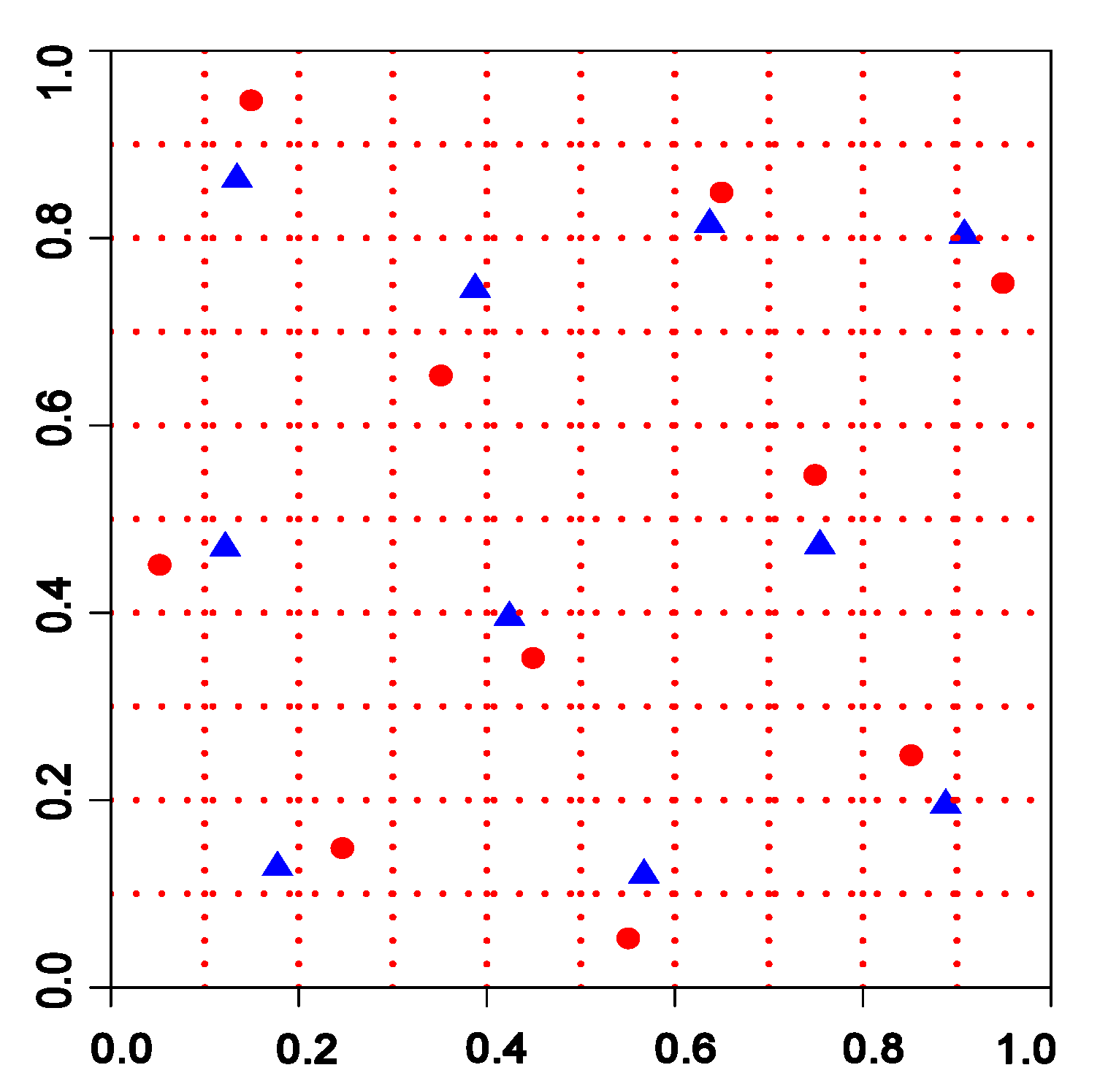
Let F be a uniform distribution on ${[0,1]}^2$ and the number of points be $n=10$. We firstly generate rep-points ${\mathcal{P}}_{SP}$ using the SP method. Under the assumption of Corollary 1, we take ${\mathcal{P}}_{SP}$ as the initial point set and ${\gamma }_{{10}^{-4},1}$ as the kernel, and generate new rep-points ${\mathcal{P}}_{PEKD}$ with the algorithm proposed in Section 3. Figure 2 shows the scatter plot of these two rep-points sets.

From Figure 2, rep-points (●) based on kernel ${\gamma }_{{10}^{-4},1}$ is indeed a central Latin hypercube design, which has great one-dimensional projection. Observing carefully, these circular points can be observed as the result of moving the triangular points to the center of the grid while keeping the rank of the triangular points in each dimension unchanged. This rank-preserving sampling technique is known as Latin hypercube sampling with dependence in [34,35,36].

Theorem 2.

Let F be a distribution function on the bounded region $\mathcal{X}={\mathcal{X}}_1\times \cdots \times {\mathcal{X}}_p$ with finite means, and $M={sup}_{\mathbf{x},\mathbf{y}\in \mathcal{X}}{\sum }_{k=1}^p{(x_k-y_k)}^2$. If $\theta =o(1/M)$ and $\mathbf{Y}\sim F$, then $D_{{\gamma }_{\theta ,2}}^2(F,F_{\mathcal{P}})$ can be minimized by point set ${\left\{{\mathbf{x}}_i\right\}}_{i=1}^n$ whenever $\frac{1}{n}{\sum }_{i=1}^n{\mathbf{x}}_i=\mathbb{E}\mathbf{Y}$.

Theorem 2 means that $\theta$ should not be too small in kernel ${\gamma }_{\theta ,2}$, otherwise the resulting point set would be similar to the target distribution only in the first moment. We found that the hyperparameter setting ${\theta }^{\alpha }={10}^{-4}$ works well for the numerical examples, given that the big training data ${\left\{{\mathbf{y}}_m\right\}}_{m=1}^N$ is scaled to zero mean and unit variance for each variable. The small $\alpha$ is suitable for cases where important variables are sparse. The precise selection of parameters requires a consideration of how to incorporate prior information based on the Bayesian form or sequential identification of important variables. We defer this to future work.

3. Optimization Algorithm

In this section, we introduce the successive convex approximation [28,37] framework to construct a parallel optimization algorithm to generate rep-points based on PEKD.

3.1. Successive Convex Approximation

Consider the following presumably difficult optimization problem: $\underset{\mathbf{x}\in \mathcal{X}}{min}G\left(\mathbf{x}\right),$ where the feasible set $\mathcal{X}$ is convex and $G\left(\mathbf{x}\right)$ is continuous. The basic idea of successive convex approximation (SCA) is solving a difficult problem via the sequence of simpler problems

$$\begin{array}{cc}\hfill \widehat{\mathbf{x}}\left({\mathbf{x}}^t\right)=& arg\underset{\mathbf{x}\in \mathcal{X}}{min}\tilde{G}\left(\mathbf{x}\right|{\mathbf{x}}^t),\hfill \\ \hfill {\mathbf{x}}^{t+1}=& {\mathbf{x}}^t+{\eta }^t(\widehat{\mathbf{x}}\left({\mathbf{x}}^t\right)-{\mathbf{x}}^t),\hfill \end{array}$$

(7)

where $\tilde{G}\left(\mathbf{x}\right|{\mathbf{x}}^t)$ is a surrogate of the original function $G\left(\mathbf{x}\right)$ and $\left\{{\eta }^t\right\}$ is the step size set.

Definition 5

(SCA surrogate function; [28]). A function $\tilde{G}\left(\mathbf{x}\right|\mathbf{y})$ is SCA surrogate function of $G\left(\mathbf{x}\right)$ at $\mathbf{x}=\mathbf{y}$ if it satisfies:

1 

$\tilde{G}\left(\mathbf{x}\right|\mathbf{y})$ is continuous and strongly convex about $\mathbf{x}$ for all $\mathbf{y}\in \mathcal{X}$;

2 

$\tilde{G}\left(\mathbf{x}\right|\mathbf{y})$ is differentiable about $\mathbf{x}$ and ${\nabla }_{\mathbf{x}}\tilde{G}\left(\mathbf{x}\right|\mathbf{y}){|}_{\mathbf{x}=\mathbf{y}}={\nabla }_{\mathbf{x}}G\left(\mathbf{x}\right){|}_{\mathbf{x}=\mathbf{y}}$.

Similar to gradient methods, there are three possible choices for the step size: bounded step size, backtracking line search and diminishing step size. Compared with the other two methods, the diminishing step size is more convenient in practice, so it is used in this paper. Two examples of diminishing step size rules are suggested in [28]:

• ${\eta }^{t+1}={\eta }^t(1-ϵ{\eta }^t),t=0,1,\dots$, where ${\eta }^0<1/ϵ$ and $ϵ\in (0,1)$;
• ${\eta }^{t+1}=({\eta }^t+a)/(1+b\sqrt{t}),t=0,1,\dots ,$ where $0<a\le b<1$.

3.2. Algorithm for Generating Rep-Points under PEKD

3.2.1. Algorithm Statement

Our optimization problem is to minimize the discrepancy $D_{{\gamma }_{\theta ,\alpha }}^2(F,F_{\mathcal{P}})$. Since the closed-form of the objective function is usually not available for the general distribution F, we optimized the Monte Carlo approximation version of it. Specifically, ignoring the first term and approximating the second integral with a large sample ${\left\{{\mathbf{y}}_m\right\}}_{m=1}^N$ from the distribution F in the second equation of (1); then, the optimization problem becomes

$$\underset{\mathcal{P}\subseteq \mathcal{X}}{\mathrm{argmin}}-\frac{2}{nN}\sum _{i=1}^n\sum _{m=1}^{N}exp\left\{-\sum _{k=1}^p\theta {|x_{ik}-y_{mk}|}^{\alpha }\right\}+\frac{1}{n^2}\sum _{i,j=1}^{n}exp\left\{-\sum _{k=1}^p\theta {|x_{ik}-x_{jk}|}^{\alpha }\right\}.$$

(8)

The objective function in (8) is denoted by $G({\left\{{\mathbf{x}}_i\right\}}_{i=1}^n;{\left\{{\mathbf{y}}_m\right\}}_{m=1}^N)$. We construct an appropriate surrogate function for G in the following Theorem 3.

Theorem 3

(Closed-form iterations). Let ${\left\{{\mathbf{x}}_i\right\}}_{i=1}^n, {\left\{{\mathbf{x}}_i^{\left(t\right)}\right\}}_{i=1}^n, {\left\{{\mathbf{y}}_m\right\}}_{m=1}^N\subseteq \mathcal{X}$. Assume $x_{ik}^{\left(t\right)}\ne x_{jk}^{\left(t\right)}, x_{ik}^{\left(t\right)}\ne y_{mk}$ for all $1\le i, j\le n, j\ne i, 1\le m\le N$ and $1\le k\le p$. Define the function h as:

$$\begin{array}{cc}\hfill & \tilde{G}({\left\{{\mathbf{x}}_i\right\}}_{i=1}^n;{\left\{{\mathbf{x}}_i^{\left(t\right)}\right\}}_{i=1}^n,{\left\{{\mathbf{y}}_m\right\}}_{m=1}^N)\hfill \\ \hfill =& \frac{1}{nN}\sum _{i=1}^n\sum _{m=1}^{N}exp\left\{-\sum _{k=1}^p\theta {|x_{ik}^{\left(t\right)}-y_{mk}|}^{\alpha }\right\}\left(\sum _{k=1}^p\alpha \theta {|x_{ik}^{\left(t\right)}-y_{mk}|}^{\alpha -2}{(x_{ik}-y_{mk})}^2\right)\hfill \\ \hfill & -\frac{2}{n^2}\sum _{i=1}^n\sum _{\genfrac{}{}{0pt}{}{j=1}{j\ne i}}^{n}exp\left\{-\sum _{k=1}^p\theta {|x_{ik}^{\left(t\right)}-x_{jk}^{\left(t\right)}|}^{\alpha }\right\}\left(\sum _{k=1}^p\alpha \theta {|x_{ik}^{\left(t\right)}-x_{jk}^{\left(t\right)}|}^{\alpha -2}(x_{ik}^{\left(t\right)}-x_{jk}^{\left(t\right)})(x_{ik}-x_{ik}^{\left(t\right)})\right).\hfill \end{array}$$

Then, $\tilde{G}$ is a SCA surrogate function of $G({\left\{{\mathbf{x}}_i\right\}}_{i=1}^n;{\left\{{\mathbf{y}}_m\right\}}_{m=1}^N)$ in (8) at ${\left\{{\mathbf{x}}_i^{\left(t\right)}\right\}}_{i=1}^n$. Moreover, the global minimizer of h is given by:

$$\begin{array}{cc}\hfill {\mathbf{x}}_i=& M_i\left({\left\{{\mathbf{x}}_i^{\left(t\right)}\right\}}_{i=1}^n;{\left\{{\mathbf{y}}_m\right\}}_{m=1}^N\right)={\left(\sum _{m=1}^N{\gamma }_{\theta ,\alpha }\left({\mathbf{x}}_i^{\left(t\right)},{\mathbf{y}}_m\right){\Omega }_{\theta }\right)}^{-1}\left(\sum _{m=1}^N{\gamma }_{\theta ,\alpha }\left({\mathbf{x}}_i^{\left(t\right)},\right.\right.\hfill \\ & \left.\left.{\mathbf{y}}_m\right){\Omega }_{\theta }{\mathbf{y}}_m+\frac{N}{n}\sum _{\genfrac{}{}{0pt}{}{j=1}{j\ne i}}^n{\gamma }_{\theta ,\alpha }\left({\mathbf{x}}_i^{\left(t\right)},{\mathbf{x}}_j^{\left(t\right)}\right)q\left({\mathbf{x}}_i^{\left(t\right)},{\mathbf{x}}_j^{\left(t\right)}\right)\right),\hfill \end{array}$$

(9)

where ${\gamma }_{\theta ,\alpha }\left(\mathbf{x},\mathbf{y}\right)=exp\left\{-{\sum }_{k=1}^p\theta {|x_k-y_k|}^{\alpha }\right\}$, ${\Omega }_{\theta }=\mathrm{diag}\left\{{\left(|x_{ik}^{\left(t\right)}-y_{mk}{|}^{\alpha -2}\right)}_{k=1}^p\right\}$ and

$q\left({\mathbf{x}}_i^{\left(t\right)},{\mathbf{x}}_j^{\left(t\right)}\right)={\left(|x_{ik}^{\left(t\right)}-x_{jk}^{\left(t\right)}{|}^{\alpha -2}(x_{ik}^{\left(t\right)}-x_{jk}^{\left(t\right)})\right)}_{k=1}^p$.

In order to ensure that the assumptions in Theorem 3 are satisfied and the actual calculations remain numerically stable, we add a small perturbation $\delta$ to the absolute value items in ${\Omega }_{\theta }$ and $q\left({\mathbf{x}}_i^{\left(t\right)},{\mathbf{x}}_j^{\left(t\right)}\right)$ in practice.

On the basic of the SCA algorithm framework, the construction process of rep-points under PEKD is described in Algorithm 1. If the training sample size N is too large, we can resample the mini-batch of it at each iteration, such as a mini-batch stochastic gradient descent in machine learning.

Algorithm 1: Rep-points construction algorithm under PEKD

1  Set step size $\left\{{\eta }^t\right\}\in (0,1]$;

2  Initialize $t=0$ and points set ${\mathcal{P}}^{\left(0\right)}={\left\{{\mathbf{x}}_i^{\left(0\right)}\right\}}_{i=1}^n$ with SP method;

3  repeat$\phantom{(}$

4    for $i=1,\dots ,n$ parallelly do$\phantom{(}$

5         ${\widehat{\mathbf{x}}}_i=M_i\left({\mathcal{P}}^{\left(t\right)};{\left\{{\mathbf{y}}_m\right\}}_{m=1}^N\right)$ with $M_i$ defined in (9);

6         ${\mathbf{x}}_i^{t+1}={\mathbf{x}}_i^t+{\eta }^t({\widehat{\mathbf{x}}}_i-{\mathbf{x}}_i^t)$.

7    end$\phantom{(}$

8    Update ${\mathcal{P}}^{(t+1)}={\left\{{\mathbf{x}}_i^{(t+1)}\right\}}_{i=1}^n,\mathrm{and}t\leftarrow t+1$;

9  until ${\mathcal{P}}^{\left(t\right)}$ converges;$\phantom{(}$

10  return the convergent point set ${\mathcal{P}}^{[\infty ]}$.

3.2.2. Complexity and Convergence of the Algorithm

As we can observe in Theorem 3, the surrogate function in (9) has a closed-form minimizer and optimization variables can be updated in parallel. The running time of Algorithm 1 for one loop iteration is $\mathcal{O}(\lceil n/P\rceil Np)$ such as the SP method, where P is the total number of computation cores available. As for the PSP method, assuming that a sample ${\left\{{\mathbf{\theta }}_r\right\}}_{r=1}^R$ is obtained from $\pi$ to approximate the sparsity-inducing kernel ${\gamma }_{\theta \sim \pi }(\mathbf{x},\mathbf{y})$, the one-shot algorithm in [27] takes $\mathcal{O}\left(RnNp\right)$. When the dimension p rises, R should be relatively large so that the sparsity-inducing kernel ${\gamma }_{\theta \sim \pi }(\mathbf{x},\mathbf{y})$ can be approximated well.

The following theorem gives a convergence guarantee for Algorithm 1.

Theorem 4

(Convergence of Algorithm 1). Suppose $\mathcal{X}\subseteq {\mathbb{R}}^p$ is convex and compact and assumptions in Theorem 3 hold, then every limit point set of the sequence ${\left({\mathcal{P}}^{\left(t\right)}\right)}_{t=1}^{\infty }$(at least one such point set exists) from Algorithm 1 converges to a stationary solution of (8).

4. Applications

4.1. Numerical Simulations

In this section, we compare the performance of the PEKD ($\alpha =1,1.5,2$) method with Monte Carlo (MC), inverse randomized quasi Monte Carlo (RQMC), SP and PSP methods. According to the hyperparameter setting of the PSP method in [27], we generate ${\theta }_l\stackrel{i.i.d.}{\sim }\mathrm{Gamma}(0.1,0.01)$ with small $(R=50,\mathrm{PSPs})$ and large $(R=1000,\mathrm{PSPl})$ sample size and set ${\Gamma }_{\left|\mathbf{u}\right|}^{\left(\theta \right)}=exp\{-|\mathbf{u}\left|\right\}$. PEKD and PSP methods take the point set generated by SP method as a warm start.

4.1.1. Visualization

Example 2.

Let F be the 5-dimensional i.i.d. $\mathrm{Beta}(2,4)$ distribution; we generate $n=25$ points with several sampling methods.

Figure 3 shows scattarplots and marginal histograms of the projection of the point sets on the first two dimensions. It is obvious that the sample generated by PEKD ($\alpha =1.5$) has better representation in all 1-dimensional marginal distributions and are not clustered such as in the samples obtained by SP and PSP methods on the 2-dimensional projection.

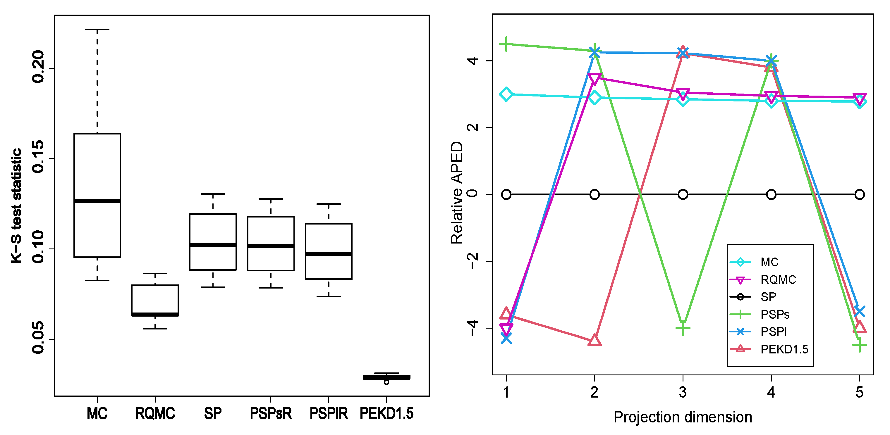
We calculate the Kolmogorov-Smirnov (K-S) test statistic between sample and $\mathrm{Beta}(2,4)$ distribution for each dimension, and average k-dimensional projected energy distance

$${\mathrm{APED}}^k=\frac{1}{\left(\genfrac{}{}{0pt}{}{5}{k}\right)}\sum _{\genfrac{}{}{0pt}{}{\mathbf{u}\subseteq \{1:5\}}{\left|\mathbf{u}\right|=k}}{D}_{{\gamma }_{ED}}^2(F^{\mathbf{u}},F_{\mathcal{P}}^{\mathbf{u}}),k=1,2,3,4,5,$$

where $\mathbf{u}$ represents the projection dimensions and $F_{\mathcal{P}}^{\mathbf{u}}$ denotes the e.d.f. of ${\left\{{\mathbf{x}}_i^{\mathbf{u}}\right\}}_{i=1}^n$. Figure 4 shows the results of two measurements (the smaller the better). PEKD method performs better on one and two dimensional projections than other methods, while the PSP method is not stable. In addition, PSP and PEKD methods sometimes perform better than the SP method in the full dimensional space; one possible reason is that they start with the rep-points generated by the SP method, which helps the SP method leave a local minimum.

4.1.2. Numerical Integration

Example 3.

Consider the approximation of integral $I={\int }_{\mathcal{X}}g\left(\mathbf{x}\right)\mathrm{d}F\left(\mathbf{x}\right)$ in [27]. Test three choices of distribution F: the i.i.d. $\mathcal{N}(0,1)$ and the i.i.d. $\mathrm{Exp}\left(1\right)$ with dimension p from 5 to 20 and two well-known integrand functions:

(1) 

Gaussian peak function $\left(\mathrm{GAPK}\right):$$g_{GAPK}\left(\mathbf{x}\right)=exp\left\{-{\sum }_{l=1}^p{a}_l^2{(x_l-u_l)}^2\right\}$,

(2) 

additive Gaussian function $\left(\mathrm{ADD}\right):$$g_{ADD}\left(\mathbf{x}\right)=exp\left\{-{\sum }_{l=1}^p{b}_l{x}_l\right\}$,

where $u_l$ is the marginal mean of $F_l$. To incorporate low-dim. structure, a fraction q of the p variables are set as active, with $a_l=b_l=0.25/\left(qp\right)$ for active variables, and 0 otherwise. These functions are denoted as $\mathrm{GPAK}\left[q\right]$ and $\mathrm{ADD}\left[q\right]$.

Some results of the integral estimation error ($log|\widehat{I}-I|$) are shown in Figure 5. In Figure 5a, there is just $pq=1$, as an important variable. PSP method with large R obtains the lower averaged error than the RQMC method at the expense of complicated calculations. It is interesting that the PEKD method ($\alpha <2$) has better performance with almost the same running time as the SP method. In Figure 5b,c, the number of important variables is small, and PEKD($\alpha =1.5$) performs best. In Figure 5d, the ratio q is large, and PEKD method with large $\alpha$ is better. In addition, the errors of RQMC method are not always lower than that of the SP method, one possible reason is that the inverse transformation method may result in a loss of the representativeness of low discrepancy sequence.

4.1.3. Uncertainty Propagation

A computer model is treated as a mathematical function g that takes varying values of input parameters denoted by a vector $\mathbf{x}\in {\mathbb{R}}^p$, and returns output $g\left(\mathbf{x}\right)$. Uncertainty propagation methods are used to estimate the distribution of model outputs resulting from a set of uncertain model outputs. In other words, let $\mathbf{X}\sim F$ denote input uncertainties; the distribution of $g\left(\mathbf{X}\right)$ can then be observed as the resulting uncertainty on the system output.

Example 4.

Three test (modified) functions are taken from [38,39]:

(1) 

$g_1\left(\mathbf{x}\right)=5+e^{-\frac{x_1^2}{2}}+e^{-\frac{x_2^2}{2}}+2cos\left(x_1\right)+2sin\left(x_2\right)$, where $x_1,x_2\stackrel{i.i.d.}{\sim }U[-1,1]$;

(2) 

$g_2\left(\mathbf{x}\right)=sin\left(x_1\right)+7{sin}^2\left(x_2\right)+0.1x_3^{4}sin\left(x_1\right)$, where $x_1,x_2,x_3\stackrel{i.i.d.}{\sim }U[-\pi ,\pi ]$;

(3) 

$g_3\left(\mathbf{x}\right)=5+x_1+0.5x_2+0.05x_3+2cos\left(20x_1\right)+0.2sin\left(20x_2\right)+2sin\left(x_3\right)$, where $x_i\stackrel{i.i.d.}{\sim }U[-1,1]$, $i=1,2,\dots ,6$.

We generate $n=60$ points with different methods to estimate the output distributions of three test functions. Figure 6 shows the K-S test statistic values (repeated 100 times) between the estimated density and the true density for each test function. SP and PEKD2 perform better on $g_1\left(\mathbf{x}\right)$ than other methods, while PSP, PEKD1 and PEKD1.5 are more suitable for $g_2\left(\mathbf{x}\right)$ and $g_3\left(\mathbf{x}\right)$. Two possible reasons are: (1) the latter two test functions are more wiggly for each dimension, which means the low-dimensional structure should be given more attention; (2) $g_3\left(\mathbf{x}\right)$ has many inactive variables, which makes SP and PEKD2 even worse than MC. In addition, the PSP method has a large variance on $g_3\left(\mathbf{x}\right)$, since its approximate sparsity-inducing kernel is unstable as the dimension increases.

4.2. Reduction of MCMC Chain

Markov Chain Monte Carlo (MCMC) is a family of techniques for the sampling probability distributions, which allows us to make statistical inferences about complex Bayesian models. If necessary, many practitioners use the thinning method (discard all but every k-th sample point after) to reduce high autocorrelation in the MCMC chain, save computer storage space and reduce processing time for computing derived posterior quantities. However, the thinning method is inefficient in most cases, since the valuable posterior samples are carelessly thrown away. Greater precision is available by working with unthinned chains. In practice, the models of interest are often high-dimensional but the desired posterior quantities involve only a handful of parameters.

Consider the orange tree growth model in [2]. The Orange data records the trunk circumference measurements $\left\{Y_i\left(t_j\right)\right\}{}_{i=1}^5{}_{j=1}^7$ of five trees (i) at seven different times ($t_j$), which can be found in R datesets package. The following hierarchical (multilevel) model is assumed in their paper:

$$\begin{array}{ccccc}\hfill & Y_i\left(t_j\right)\stackrel{indep.}{\sim }N({\eta }_i\left(t_j\right),{\sigma }_C^2),\hfill & \hfill & {\eta }_i\left(t_j\right)={\varphi }_{i1}/\left(1+{\varphi }_{i2}exp\left\{{\varphi }_{i3}{t}_j\right\}\right);\hfill & \hfill \left(\mathrm{likelihood}\right)\\ \hfill & log{\varphi }_{i1}\stackrel{indep.}{\sim }N({\mu }_1,{\sigma }_1^2),\hfill & \hfill & log({\varphi }_{i2}+1)\stackrel{indep.}{\sim }N({\mu }_2,{\sigma }_2^2),\hfill & \\ \hfill & log(-{\varphi }_{i3})\stackrel{indep.}{\sim }N({\mu }_3,{\sigma }_3^2),\hfill & \hfill & {\sigma }_C^2\sim \text{Inv-Gamma}(0.001,0.001);\hfill & \hfill \left(\mathrm{priors}\right)\\ \hfill & {\mu }_k\stackrel{i.i.d.}{\sim }N(0,100),\hfill & \hfill & {\sigma }_k^2\stackrel{i.i.d.}{\sim }\text{Inv-Gamma}(0.01,0.01);\hfill & \hfill \left(\mathrm{hyperpriors}\right)\\ \hfill & i=1,\dots ,5,j=1,\dots ,7\mathrm{and}k=1,2,3.\hfill & \hfill & \end{array}$$

The parameter set of interest is $\Theta =({\varphi }_{11},{\varphi }_{12},\dots ,{\varphi }_{53},{\sigma }^2)$. As suggested in [2], we generate the chain with 150,000 iterations and the first half of the sample is discarded as a burn-in based on the R package rstan. Then, the full chain (N = 75,000) is compressed to a small sample ($n=375$) with thinning, SP, PSPs and PEKD($\alpha =1.5,2$) methods. Compare these methods on how well they estimate (a) the marginal posterior means and variances of each parameter, (b) the averaged instantaneous growth rate $r\left(t\right)=\frac{1}{5}{\sum }_{i=1}^5{\left.\frac{\partial }{\partial s}{\eta }_i\left(s\right)\right|}_{s=t}$ at three future times (t = 1600, 1625, 1650). True posterior quantities are estimated by running a longer MCMC chain with 600,000 iterations.

Table 1. The error ratios of thinning method over SP, PSP and PEKD methods in estimating the posterior quantities. The larger, the better.

Parameter	Estimations of Quantities with Different Methods
	Means				Variances
	SP	PSPs	PEKD1.5	PEKD2	SP	PSPs	PEKD1.5	PEKD2
${\varphi }_{i1}$	21.00	21.43	21.49	21.60	2.72	2.61	4.33	3.21
${\varphi }_{i2}$	8.78	8.74	10.18	9.17	3.79	3.43	4.03	3.30
${\varphi }_{i3}$	7.00	7.33	8.71	7.17	4.27	4.12	5.31	3.63
${\sigma }_C^2$	24.17	27.48	42.25	44.40	5.04	5.68	11.64	5.82
r(1600)	14.00	15.79	26.72	30.27	-	-	-	-
r(1625)	12.85	14.29	24.04	25.16	-	-	-	-
r(1650)	11.90	13.09	21.90	21.61	-	-	-	-

reports the error ratios of the thinning method over SP, PSPs and PEKD methods in estimating the posterior quantities of interest. The larger the ratio is, the more accurate the estimation is. From Table 1, compared with the thinning method, other methods can estimate parameters more accurately. The PEKD1.5 method is stable and performs best for most parameter estimates, while PEKD2 method performs well only in the estimation of the mean value.

5. Conclusions and Discussion

In this work, a new rep-points criterion named PEKD is introduced. The most attractive property of PEKD is that the low-dimensional representativeness of rep-points can be regulated by tuning the hyperparameter $\alpha$. The smaller the $\alpha$, the lower the dimensional representative will be assured primarily. Actually, when $\alpha =1$, the rep-points under the PEKD is an LHD for uniform distribution on ${[0,1]}^p$, which means the 1-dimensional representativeness achieves the best performance. What is more, a parallelized optimization algorithm is also constructed for generating the rep-points under the criterion PEKD. Simulation studies and an example of real data demonstrate that PEKD with small $\alpha$ is suitable for situations where important variables are sparse and the function fluctuates greatly, and $\alpha =1.5$ is a robust choice in most cases.

As a general distribution similarity measure, PEKD can be used to test independence and goodness-of-fit [31,40,41,42]. For the experimental design community, PEKD can be used as a criterion to construct complex designs, such as space-filling design and sliced design [16,43,44,45] in the irregular region. In addition, the algorithm proposed in this paper would be helpful for data splitting [46] and model-free subsampling [47] problems in the machine learning community.

References

1. Flury, B.A. Principal Points. Biometrika 1990, 77, 33–41. [Google Scholar] [CrossRef]
2. Mak, S.; Joseph, V.R. Support points. Ann. Stat. 2018, 46, 2562–2592. [Google Scholar] [CrossRef]
3. Anderberg, M.R. Cluster Analysis for Applications; Academic Press: San Diego, CA, USA, 1973. [Google Scholar] [CrossRef]
4. Fang, K.T.; He, S.D. The Problem of Selecting a Given Number of Representative Points in a Normal Population and a Generalized Mills’ Ratio; Technical Report; Stanford University, Department of Statistics: Stanford, CA, USA, 1982. [Google Scholar] [CrossRef]
5. Flury, B.D. Estimation of principal points. J. R. Stat. Soc. Ser. C Appl. Stat. 1993, 42, 139–151. [Google Scholar] [CrossRef]
6. Fang, K.; Zhou, M.; Wang, W. Applications of the representative points in statistical simulations. Sci. China Math. 2014, 57, 2609–2620. [Google Scholar] [CrossRef]
7. Lemaire, V.; Montes, T.; Pagès, G. New weak error bounds and expansions for optimal quantization. J. Comput. Appl. Math. 2020, 371, 112670. [Google Scholar] [CrossRef] [Green Version]
8. Mezic, I.; Runolfsson, T. Uncertainty propagation in dynamical systems. Automatica 2008, 44, 3003–3013. [Google Scholar] [CrossRef]
9. Mohammadi, S.; Cremaschi, S. Efficiency of Uncertainty Propagation Methods for Estimating Output Moments. In Proceedings of the 9th International Conference on Foundations of Computer-Aided Process Design, 14–18 July 2019, Copper Mountain, CO, USA; Muñoz, S.G., Laird, C.D., Realff, M.J., Eds.; Elsevier: Amsterdam, The Netherlands, 2019; Volume 47, pp. 487–492. [Google Scholar] [CrossRef]
10. Owen, A.B. Statistically Efficient Thinning of a Markov Chain Sampler. J. Comput. Graph. Stat. 2017, 26, 738–744. [Google Scholar] [CrossRef]
11. Riabiz, M.; Chen, W.Y.; Cockayne, J.; Swietach, P.; Niederer, S.A.; Mackey, L.; Oates, C.J. Optimal thinning of MCMC output. J. R. Stat. Soc. Ser. B 2022, 84, 1059–1081. [Google Scholar] [CrossRef]
12. South, L.F.; Riabiz, M.; Teymur, O.; Oates, C.J. Postprocessing of MCMC. Annu. Rev. Stat. Its Appl. 2022, 9, 529–555. [Google Scholar] [CrossRef]
13. Xu, L.H.; Fang, K.T.; Pan, J. Limiting behavior of the gap between the largest two representative points of statistical distributions. Commun. Stat.-Theory Methods 2021, 1–24. [Google Scholar] [CrossRef]
14. Li, Y.; Fang, K.T.; He, P.; Peng, H. Representative Points from a Mixture of Two Normal Distributions. Mathematics 2022, 10, 3952. [Google Scholar] [CrossRef]
15. Xu, L.H.; Fang, K.T.; He, P. Properties and generation of representative points of the exponential distribution. Stat. Pap. 2022, 63, 197–223. [Google Scholar] [CrossRef]
16. Fang, K.T.; Liu, M.Q.; Qin, H.; Zhou, Y.D. Theory and Application of Uniform Experimental Designs; Springer: Singapore, 2018. [Google Scholar] [CrossRef]
17. Pronzato, L.; Zhigljavsky, A. Bayesian quadrature, energy minimization and space-filling design. SIAM/ASA J. Uncertain. Quantif. 2020, 8, 959–1011. [Google Scholar] [CrossRef]
18. Borodachov, S.; Hardin, D.; Saff, E. Low Complexity Methods for Discretizing Manifolds via Riesz Energy Minimization. Found. Comput. Math. 2014, 14, 1173–1208. [Google Scholar] [CrossRef] [Green Version]
19. Joseph, V.R.; Dasgupta, T.; Tuo, R.; Wu, C.F.J. Sequential Exploration of Complex Surfaces Using Minimum Energy Designs. Technometrics 2015, 57, 64–74. [Google Scholar] [CrossRef]
20. Goodfellow, I.; Bengio, Y.; Courville, A. Deep Learning; MIT Press: Cambridge, MA, USA, 2016. [Google Scholar]
21. Yang, Q.; Zhang, Y.; Dai, W.; Pan, S.J. Transfer Learning; Cambridge University Press: Cambridge, UK, 2020. [Google Scholar] [CrossRef]
22. Fang, K.T.; Wang, Y. Number-Theoretic Methods in Statistics; Chapman and Hall: London, UK, 1994. [Google Scholar]
23. Briol, F.X.; Oates, C.J.; Girolami, M.; Osborne, M.A.; Sejdinovic, D. Probabilistic Integration: A Role in Statistical Computation? Stat. Sci. 2019, 34, 1–22. [Google Scholar] [CrossRef] [Green Version]
24. Chen, Y.; Welling, M.; Smola, A.J. Super-Samples from Kernel Herding. arXiv 2012, arXiv:1203.3472. [Google Scholar] [CrossRef]
25. Hickernell, F.J. A generalized discrepancy and quadrature error bound. Math. Comput. 1998, 67, 299–322. [Google Scholar] [CrossRef] [Green Version]
26. Zhou, Y.D.; Fang, K.T.; Ning, J.H. Mixture discrepancy for quasi-random point sets. J. Complex. 2013, 29, 283–301. [Google Scholar] [CrossRef]
27. Mak, S.; Joseph, V.R. Projected support points: A new method for high-dimensional data reduction. arXiv 2018, arXiv:1708.06897. [Google Scholar] [CrossRef]
28. Scutari, G.; Sun, Y. Parallel and Distributed Successive Convex Approximation Methods for Big-Data Optimization. In Multi-Agent Optimization: Cetraro, Italy 2014; Facchinei, F., Pang, J.S., Eds.; Springer International Publishing: Cham, Switzerland, 2018; pp. 141–308. [Google Scholar] [CrossRef] [Green Version]
29. Santner, T.J.; Williams, B.J.; Notz, W.I. The Design and Analysis of Computer Experiments; Springer: New York, NY, USA, 2018. [Google Scholar] [CrossRef]
30. N’Gbo, N.; Tang, J. On the Bounds of Lyapunov Exponents for Fractional Differential Systems with an Exponential Kernel. Int. J. Bifurc. Chaos 2022, 32, 2250188. [Google Scholar] [CrossRef]
31. Székely, G.J.; Rizzo, M.L. Energy statistics: A class of statistics based on distances. J. Stat. Plan. Inference 2013, 143, 1249–1272. [Google Scholar] [CrossRef]
32. Fang, K.T.; Hickernell, F.J. Uniform Experimental Designs; Springer: New York, NY, USA, 2007. [Google Scholar] [CrossRef]
33. Lange, K. MM Optimization Algorithms; SIAM: Philadelphia, PA, USA, 2016. [Google Scholar] [CrossRef]
34. Stein, M.L. Large sample properties of simulations using latin hypercube sampling. Technometrics 1987, 29, 143–151. [Google Scholar] [CrossRef]
35. Packham, N.; Schmidt, W.M. Latin hypercube sampling with dependence and applications in finance. J. Comput. Financ. 2010, 13, 81–111. [Google Scholar] [CrossRef] [Green Version]
36. Aistleitner, C.; Hofer, M.; Tichy, R.F. A central limit theorem for Latin hypercube sampling with dependence and application to exotic basket option pricing. Int. J. Theor. Appl. Financ. 2012, 15, 1–20. [Google Scholar] [CrossRef] [Green Version]
37. Scutari, G.; Facchinei, F.; Song, P.; Palomar, D.P.; Pang, J.S. Decomposition by Partial Linearization: Parallel Optimization of Multi-Agent Systems. IEEE Trans. Signal Process. 2014, 62, 641–656. [Google Scholar] [CrossRef] [Green Version]
38. Oakley, J.E.; O’Hagan, A. Bayesian inference for the uncertainty distribution of computer model outputs. Biometrika 2002, 89, 769–784. [Google Scholar] [CrossRef] [Green Version]
39. Marrel, A.; Iooss, B.; Laurent, B.; Roustant, O. Calculations of sobol indices for the gaussian process metamodel. Reliab. Eng. Syst. Saf. 2009, 94, 742–751. [Google Scholar] [CrossRef] [Green Version]
40. Székely, G.J.; Rizzo, M.L.; Bakirov, N.K. Measuring and testing dependence by correlation of distances. Ann. Stat. 2007, 35, 2769–2794. [Google Scholar] [CrossRef]
41. Wang, S.; Liang, J.; Zhou, M.; Ye, H. Testing Multivariate Normality Based on F-Representative Points. Mathematics 2022, 10, 4300. [Google Scholar] [CrossRef]
42. Liang, J.; He, P.; Yang, J. Testing Multivariate Normality Based on t-Representative Points. Axioms 2022, 11, 587. [Google Scholar] [CrossRef]
43. Xiong, Z.K.; Liu, W.J.; Ning, J.H.; Qin, H. Sequential support points. Stat. Pap. 2022, 63, 1757–1775. [Google Scholar] [CrossRef]
44. Xiao, Y.; Ning, J.H.; Xiong, Z.K.; Qin, H. Batch sequential adaptive designs for global optimization. J. Korean Stat. Soc. 2022, 51, 780–802. [Google Scholar] [CrossRef]
45. Kong, X.; Zheng, W.; Ai, M. Representative points for distribution recovering. J. Stat. Plan. Inference 2023, 224, 69–83. [Google Scholar] [CrossRef]
46. Joseph, V.R.; Vakayil, A. Split: An optimal method for data splitting. Technometrics 2022, 64, 166–176. [Google Scholar] [CrossRef]
47. Zhang, M.; Zhou, Y.; Zhou, Z.; Zhang, A. Model-free Subsampling Method Based on Uniform Designs. arXiv 2022, arXiv:2209.03617. [Google Scholar] [CrossRef]
Figure 1. Contours of different kernels. (a) Negative Euclidean distance kernel in support points (SP) method; (b) Gaussian kernel; (c) sparsity-inducing kernel in projected support points (PSP) method; (df) power exponential (PE) kernel with α = 0.5 , 1 , 1.5 , respectively. The point A and point B in all figures have the same coordinates in the second dimension, and x A x B 2 = x A x C 2 .
Axioms 11 00711 g001
Figure 2. Scatterplots of rep-points for uniform distribution on [ 0 , 1 ] 2 generated by SP method () and PEKD method ().
Axioms 11 00711 g002
Figure 3. Scattarplots and marginal histograms of n = 25 points for 5-dimensional i.i.d Beta(2,4) with six samplers. Red lines represent the true marginal densities. (a) MC; (b) RQMC; (c) SP; (d) PSPs; (e) PSPl; (f) PEKD1.5.
Axioms 11 00711 g003
Figure 4. Box plots of K-S test statistic and relative average projected energy distance (setting SP method as a benchmark by calculating sign ( APED SP k APED method k ) log 10 ( | APED SP k APED method k | ) ).
Axioms 11 00711 g004
Figure 5. Box plots of Log-Error for GAPK and ADD under p dimensional i.i.d. N ( 0 ,   1 ) and Exp ( 1 ) . (a) Normal ( GAPK [ 0.2 ] , n = 50 , p = 5 ); (b) Normal ( GAPK [ 0.2 ] , n = 50 , p = 20 ); (c) Exp ( ADD [ 0.1 ] , n = 100 ,   p = 20 ) ; (d) Exp ( ADD [ 0.4 ] , n = 100 ,   p = 20 ) .
Axioms 11 00711 g005
Figure 6. Box plots of K-S test statistic for three test functions on uncertainty propagation of computer experiments. The smaller, the better. (a) g 1 ( x ) ; (b) g 2 ( x ) ; (c) g 3 ( x ) .
Axioms 11 00711 g006