Article

Hyperbolic B-Spline Function-Based Differential Quadrature Method for the Approximation of 3D Wave Equations

Department of Mathematics, College of Science, Jazan University, Jazan 45142, Saudi Arabia
*
Author to whom correspondence should be addressed.
Axioms 2022, 11(11), 597; https://doi.org/10.3390/axioms11110597
Submission received: 24 September 2022 / Revised: 17 October 2022 / Accepted: 20 October 2022 / Published: 28 October 2022
(This article belongs to the Special Issue Mathematical Modelling and Applications)

Abstract

:
We propose a differential quadrature method (DQM) based on cubic hyperbolic B-spline basis functions for computing 3D wave equations. This method converts the problem into a system of ODEs. We use an optimum five-stage and order four SSP Runge-Kutta (SSPRK-(5,4)) scheme to solve the obtained system of ODEs. The matrix stability analysis is also investigated. The accuracy and efficiency of the proposed method are demonstrated via three numerical examples. It has been found that the proposed method gives more accurate results than the existing methods. The main purpose of this work is to present an accurate, economically easy-to-implement, and stable technique for solving hyperbolic partial differential equations.

1. Introduction

Some of the existing numerical approaches for solving wave equations as well as fractional wave equations involve the temporal extrapolation method, finite difference method (FDM), finite volume method (FVM), finite element method (FEM), and boundary element method (BEM) [1,2,3,4,5]. It has been noticed that the most popularly used numerical approaches for solving 3D wave equations are based on the FDM [6,7]. In short, the FDM is utilized to handle the time derivative, and the space derivatives are discretized by other numerical techniques. In particular, the radial basis and B-spline basis functions-based collocation methods are extensively applied for solving 3D wave equations. Ranocha et al. [8] set up fully discrete conservative techniques for various disseminative wave equations. Recently, Wang et al. [9] presented radial basis function-based single-step mesh free technique for 2D variable coefficients wave equation. Bakushinsky and Leonov [10] presented a fast Fourier transform-based algorithm to solve the 3D wave inverse problem in a cylindrical system.
In recent decades, wave equations have been approximated by numerous researchers. Dehghan [11] approximated the solution of 1D hyperbolic PDEs with nonlocal boundary specifications, while in [12], the author used ADI, fully implicit, fully explicit FD methods, and the Barakat and Clark type explicit formulae to approximate the 2D Schrodinger equation. Mohanty and Gopal [13] presented an off-step discretization-based technique for the approximation of 3D wave equations. Titarev and Toro [14] implemented fourth-order accurate ADER schemes for 3D hyperbolic systems. Zhang et al. [15] proposed an improved element-free Galerkin (EFG) method, while EFG method and Meshless local Petrov-Galerkin (MLPG) method have been proposed by Shivanian [16]. Recently, Shukla et al. [17] proposed an Expo-MCBDQM to approximate the aforementioned equations.
Bellman et al. [18] introduced DQM. DQM based on various basis functions has been presented to solve several PDEs such as sinc DQM [19], Fourier expansion based DQM [20], harmonic DQM [21], quintic B-spline DQM [22] and many more. The authors of [23,24,25,26] proposed a cubic B-spline (CB-spline) based DQM for the Burgers’, coupled Burgers’, Sine-Gordon, and advection-diffusion equations, respectively while the authors of [27] proposed an exponential CB-spline based DQM for the Burgers’ equation. The authors of [28] proposed a polynomial differential quadrature method to solve the two-dimensional Sine-Gordon equation. Korkmaz and Dag [29] proposed CB-Spline based DQMs to simulate the boundary forced RLW equation, while in [30], they proposed Quartic as well as quintic B-spline based differential quadrature methods for the advection-diffusion equation. Jiwari [31] proposed Lagrange interpolation as well as CB-spline based DQMs to solve the hyperbolic PDEs. The authors in [32] presented a new cubic B-spline-based semi-analytical method for solving 3D anisotropic convention-diffusion-reaction problems. Ali et al. [33] considered nonlinear spin dynamics in Heisenberg ferromagnetic spin chain mode for solving travelling waves using the unified method.
Recently, a modified auxiliary equation mapping method was applied to study the new exact travelling and solitary wave solutions of the coupled Whitham-Broer-Kaup, (2+1)-dimensional Broer-Kaup-Kupershmit and Drinfel’d-Sokolow-Wilson equations [34]. Seadawy et al. [35] studied a new modified 3-dimentional fractional Benjamin-Bona-Mahony equations by using conformable fractional order derivatives in both spatial and temporal variables. Furthermore, in [36], an extended modified auxiliary equation mapping method was used highlight the solutions for the 3D fractional WBBM equation.
B-spline basis functions have several interesting properties and are the basis of the vector space generated by the spline with minimal support and with respect to a certain degree of smoothness and domain partition. Ahlberg et al. [37] considered cubic splines with a deficiency of 2 in the real domain, satisfying the condition that they should be easily constructed, and the error between them and the given function as well as those between their derivatives must easily allow for accurate estimates, although they did not work on the error bounds in detail. Lu [38] suggested using interpolated complex cubic splines with a deficiency of 2 with advantages over those with a deficiency of 1 in that it is much easier to construct them and much easier to estimate the error bounds.
Motivated by the aforementioned work, we propose a DQM based on hyperbolic B-spline functions to approximate the 3D wave equations. All geometric characteristics of the proposed hyperbolic B-spline curves are similar to the classical B-spline, but the shape adjustability is an additional quality that the classical B-spline curves do not hold. The main purpose of this work is to present an accurate, economically easy-to-implement, and stable technique for solving hyperbolic partial differential equations. We consider
2 u t 2 + ( α 1 δ f ( u ) ) u t = 2 u x 2 + 2 u y 2 + 2 u z 2 α 2 u + p ^ ( x , y , z , t ) ,   ( x , y , z ) Ω ,
with
u | t = 0 = ξ 1 ,   and   u t | t = 0 = ξ 2 ,
and with boundary conditions
u ( x , y , z , t ) = ζ ,   ( x , y , z ) Ω ,
where Ω = { ( x , y , z ) : x , y , z [ 0 , 1 ] } is the problem domain and Ω is its boundary. The functions f , ξ 1 , ξ 2 and ζ are known whereas u = u ( x , y , z , t ) is to be determined. The terms α 1 , α 2 , δ are real constants.
The rest of the paper is organized as follows. In Section 2, the procedure of the cubic hyperbolic B-spline DQM is described. Section 3 examines the stability analysis of the proposed method. Section 4 demonstrates the computational results. Finally, Section 5 presents the conclusion of our study.

2. The Hyperbolic B-Spline Differential Quadrature Method

In this section, we consider the problem (1)–(3) when α 1 , α 2 , δ , f ( u ) , p are known and u is to be evaluated. We apply the cubic hyperbolic B-spline DQM to approximate 3D wave Equations (1)–(3). First, we split Ω = { ( x , y , z ) : 0 x , y , z 1 } into equal length mesh h x = 1 M x 1 , h y = 1 M y 1 and h z = 1 M z 1 . For discrete form, we denote u i j k = u ( x i , y j , z k , t ) , i = 1 , 2 , , M x ,   j = 1 , 2 , , M y and k = 1 , 2 , , M z .
In DQM, we approximate u x x , u y y and u z z as given below:
p u i j k x p = r = 1 M x a i r ( p ) u r j k ,   i = 1 , 2 , , M x ,
p u i j k y p = r = 1 M y b j r ( p ) u i r k ,   j = 1 , 2 , , M y ,
p u i j k z p = r = 1 M z c k r ( p ) u i j r ,   k = 1 , 2 , , M z ,
where u i j k = u ( x i , y j , z k , t ) , and a i r ( p ) , b j r ( p ) , c k r ( p ) are the weighting coefficients corresponding to p u i j k x p ,   p u i j k y p and p u i j k z p , respectively, at time t .
The cubic hyperbolic B-spline functions are given as [39]:
H f i ( x ) = { ( S i 2 ) 3 sinh ( 3 h ) sinh ( 2 h ) sinh ( h ) ,   [ x i 2 , x i 1 ) , S i ( S i 2 ) 2 S i + 1 S i 1 S i 2 S i + 2 ( S i 1 ) 2 sinh ( 3 h ) sinh ( 2 h ) sinh ( h ) , [ x i 1 , x i ) , S i 2 ( S i + 2 ) 2 + S i + 2 S i + 1 S i 1 + S i ( S i + 2 ) 2 sinh ( 3 h ) sinh ( 2 h ) sinh ( h ) , [ x i , x i + 1 ) , ( S i + 2 ) 3 sinh ( 3 h ) sinh ( 2 h ) sinh ( h ) ,   [ x i + 1 , x i + 2 ) , 0 ,   otherwise ,
where S i = sinh ( x x i )   and   h = x i + 1 x i .
The cubic hyperbolic B-spline functions { H f 0 , H f 1 , , H f M , H f M + 1 } form a basis over Ω . Table 1 shows the values of cubic hyperbolic B-spline functions with derivatives at the knots, where
ϒ 1 = ϒ 3 = ( sinh ( h ) ) 3 sinh ( 3 h ) sinh ( 2 h ) sinh ( h ) ,   ϒ 2 = 2 sinh ( 2 h ) ( sinh ( h ) ) 2 sinh ( 3 h ) sinh ( 2 h ) sinh ( h ) , ϒ 4 = 3 2 sinh ( 3 h ) ,   ϒ 5 = 3 2 sinh ( 3 h ) .
Preserving the matrix system remains diagonally dominant, we modify the hyperbolic B-spline functions as:
H ^ f 1 ( x ) = H f 1 ( x ) + 2 H f 0 ( x ) H ^ f 2 ( x ) = H f 2 ( x ) H f 0 ( x ) H ^ f m ( x ) = H f m ( x )   for   m = 3 , , M x 2 H ^ f M x 1 ( x ) = H f M x 1 ( x ) H f M x + 1 ( x ) H ^ f M x ( x ) = H f M x ( x ) + 2 H f M x + 1 ( x ) } ,
where the modified cubic hyperbolic B-spline functions { H ^ f 1 ,   H ^ f 2 ,   , H ^ f M x } form basis over Ω . Next, in u i j k x , we use the modified basis functions H ^ f r ( x ) , r = 1 , 2 , , M x in (4) to evaluate a i j ( 1 ) . Then, Equation (4) yields
H ^ f r ( x i ) = q = 1 M x a i q ( 1 ) H ^ f r ( x q ) ,   i = 1 , 2 , , M x ,
which can be written in the form of tridiagonal system as follows:
A x [ i ] = B [ i ] ,   for   i = 1 , 2 , , M x ,
where A = [ H ^ f i j ] is the M x × M x matrix given by
A = [ ϒ 2 + 2 ϒ 1 ϒ 3 0 0 0 0 ϒ 1 ϒ 3 ϒ 2 ϒ 3 0 0 0 0 ϒ 1 ϒ 2 ϒ 3 0 0 0 0 ϒ 1 ϒ 2 ϒ 3 0 0 0 0 ϒ 1 ϒ 2 ϒ 3 ϒ 1 0 0 0 0 ϒ 1 ϒ 1 + 2 ϒ 1 ] ,
x [ i ] = [ a i 1 ( 1 ) , a i 2 ( 1 ) , , a i M x ( 1 ) ] T is the unknown vector and
B [ 1 ] = [ 2 ϒ 5 ϒ 4 ϒ 5 0 0 0 0 ] ,   B [ 2 ] = [ ϒ 5 0 ϒ 4 0 0 0 ] ,   ,   B [ M x 1 ] = [ 0 0 0 ϒ 5 0 ϒ 5 ] ,   B [ M x ] = [ 0 0 0 0 ϒ 5 ϒ 4 2 ϒ 4 ] .
We solve the system (10) to find the weighting coefficient vector a i j ( 1 ) . Similarly, by fixing x and z in u i j k y and using the modified cubic hyperbolic B-spline functions H ^ f r ( y ) , r = 1 , 2 , , M x in Equation (5), and fixing x and y in u i j k z and using the modified cubic hyperbolic B-spline functions H ^ f r ( z ) , r = 1 , 2 , , M x in Equation (6), we can compute b i j ( 1 ) and c i j ( 1 ) .
Next, for computing a i j ( p ) ,   b i j ( p ) and c i j ( p ) , we use the Shu’s [40] recurrence relations
a i j ( p ) = p ( a i j ( 1 ) a i i ( p 1 ) a i j ( p 1 ) x i x j ) ,   if   j i ; a i i ( p ) = j = 1 , j i M x a i j ( p ) ,   for   i , j = 1 , 2 , , M x ,
b i j ( p ) = p ( b i j ( 1 ) b i i ( p 1 ) b i j ( p 1 ) y i y j ) ,   if   j i ; b i i ( p ) = j = 1 , j i M y b i j ( p ) ,   for   i , j = 1 , 2 , , M y ,
c i j ( p ) = p ( c i j ( 1 ) c i i ( p 1 ) c i j ( p 1 ) z i z j ) ,   if   j i ; c i i ( p ) = j = 1 , j i M z c i j ( p ) ,   for   i , j = 1 , 2 , , M z .
Now, using u t = w , u t t = w t and substituting the approximated u x x ,   u y y and u z z by the cubic hyperbolic B-spline DQM in problem (1) and (2), we have
d u i j k d t = w i j k ,
and
d w i j k d t = r = 1 M x a i r ( 2 ) u r j k + r = 1 M y b j r ( 2 ) u i r k + r = 1 M z c k r ( 2 ) u i j r ( α 1 δ f ( u i j k ) ) w i j k α 2 u i j k + P ¯ i j k ,
where i = 0 , 1 , , M x ,   j = 0 , 1 , , M y ,   k = 0 , 1 , , M z , . Using Equation (3) in the above equation, we have
d u i j k d t = w i j k ,
and
d w i j k d t = r = 2 M x 1 a i r ( 2 ) u r j k + r = 2 M y 1 b j r ( 2 ) u i r k + r = 2 M z 1 c k r ( 2 ) u i j r ( α 1 δ f ( u i j k ) ) w i j k α 2 u i j k + P ¯ i j k ,
where,
P ¯ i j k = a i 1 ( 2 ) u 1 j k + a i M x ( 2 ) u M x j k + b j 1 ( 2 ) u i 1 k + b j M y ( 2 ) u i M y k + c k 1 ( 2 ) u i j 1 + c k M z ( 2 ) u i j M z + p ^ i j k .
Finally, we apply SSPRK-(5,4) scheme [41] to solve the above systems.

3. Stability Analysis

For stability, we rewrite Equations (16) and (17) by choosing α 1 , α 2 0 and α 1 > δ f as follows:
d X d t = A ^ X + X ^ ,
where, X = [ u w ] t r , X ^ = [ N P ¯ ] t r , A ^ = [ N I F ( α 1 + δ f ) I ] , N and I are null and identity matrices, respectively. We have F = F x + F y + F z α 2 I where F x ,   F y and F z are ( M x 2 ) ( M y 2 ) ( M z 2 ) order matrices for a i j ( 2 ) ,   b i j ( 2 ) and c i j ( 2 ) , respectively, and given as follows:
F x = [ a 22 ( 2 ) I x a 23 ( 2 ) I x a 2 ( M x 1 ) ( 2 ) I x a 32 ( 2 ) I x a 33 ( 2 ) I x a 3 ( M x 1 ) ( 2 ) I x a ( M x 1 ) 2 ( 2 ) I x a ( M x 2 ) 3 ( 2 ) I x a ( M x 1 ) ( M x 1 ) ( 2 ) I x ] ,
  F y = [ X ˜ y N y N y N y X ˜ y N y N y N y X ˜ y ] ; X ˜ y = [ b 22 ( 2 ) I z b 23 ( 2 ) I z b 2 ( M y 1 ) ( 2 ) I z b 32 ( 2 ) I z b 33 ( 2 ) I z b 3 ( M y 1 ) ( 2 ) I z b ( M y 1 ) 2 ( 2 ) I z b ( M y 2 ) 3 ( 2 ) I z b ( M y 1 ) ( M y 1 ) ( 2 ) I z ] ,
  F z = [ X ˜ z N z N z N y X ˜ z N z N z N z X ˜ z ] ; X ˜ y = [ c 22 ( 2 ) I z c 23 ( 2 ) I z c 2 ( M z 1 ) ( 2 ) I z c 32 ( 2 ) I z c 33 ( 2 ) I z c 3 ( M z 1 ) ( 2 ) I z c ( M z 1 ) 2 ( 2 ) I z c ( M z 2 ) 3 ( 2 ) I z c ( M z 1 ) ( M z 1 ) ( 2 ) I z ] .
The order of null matrices N y and N z are ( M y 2 ) ( M z 2 ) and ( M z 2 ) , respectively which is same as the order of identity matrices I x and I z .
Now, we suppose that λ A be an eigenvalue of A associated with the eigenvector ( X 1 ,   X 2 ) t r , where the order of each component vector is ( M x 2 ) ( M y 2 ) ( M z 2 ) . Then, we have
[ O I F ( α 1 + δ f ) I ] [ X 1 X 2 ] = λ A [ X 1 X 2 ] ,
which implies that I X 2 = λ A X 1 and F X 1 ( α 1 δ f ) X 2 = λ A X 2 .
Thus, we have
F X 1 = λ A ( λ A + α 1 δ f ) X 1 .
This illustrates that λ A ( λ A + α 1 δ f ) is the eigenvalue of F as follows:
F = α 2 I + F 1 .
The eigenvalues of F 1 with h x = h y = h z = 0.2, 0.1 and 0.05 are represented in Figure 1, where real and negative eigenvalues are observed. Equation (25) implies that all eigenvalues of B are real and negative.
Now, let λ A = x + i y , then we have ( λ A + α 1 δ f ) λ A = ( x 2 + ( α 1 δ f ) x y 2 ) + i ( 2 x + ( α 1 δ f ) ) y is negative and real, that is,
x 2 + ( α 1 δ f ) x y 2 < 0   and   2 x y + ( α 1 δ f ) y = 0 .
From Equation (26), we conclude that x = 0.5 ( α 1 δ f ) if y 0 and x < ( α 1 δ f ) if y = 0 . Since α 1 > δ f and so x < 0 , we conclude that the real part of λ A will be negative. Therefore, the proposed method is stable for the 3D wave equations discretized system.

4. Computational Results

Now, we consider three examples of the 3D wave Equation (1) to check the accuracy and efficiency of the proposed method.
Example 1.
We consider Equation (1) for δ = 0 and α i = 2 ,   i = 1 , 2 with the analytical solution u ( x , y , z , t ) = e - 2 t sinh x   sinh y   sinh z .
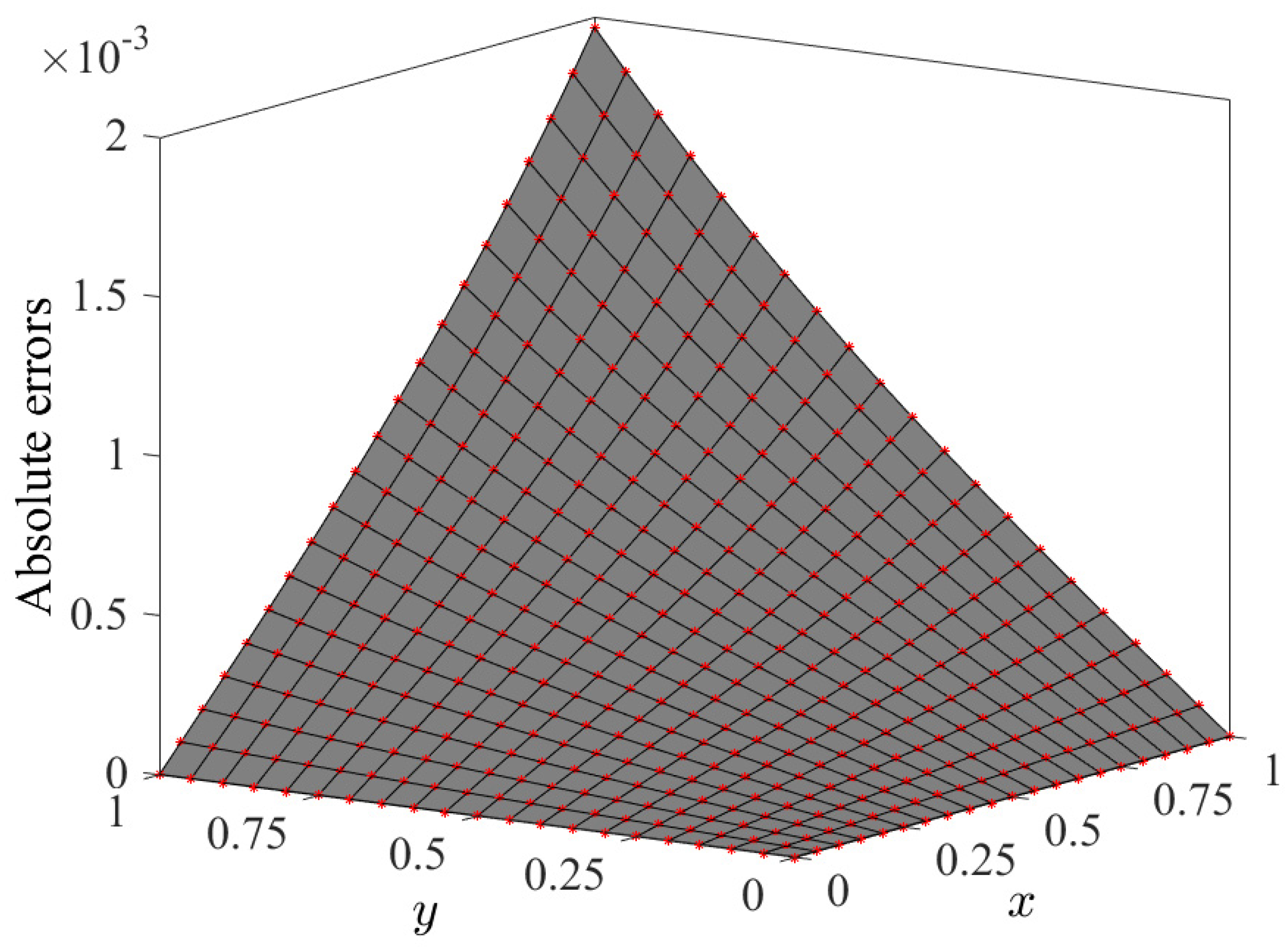
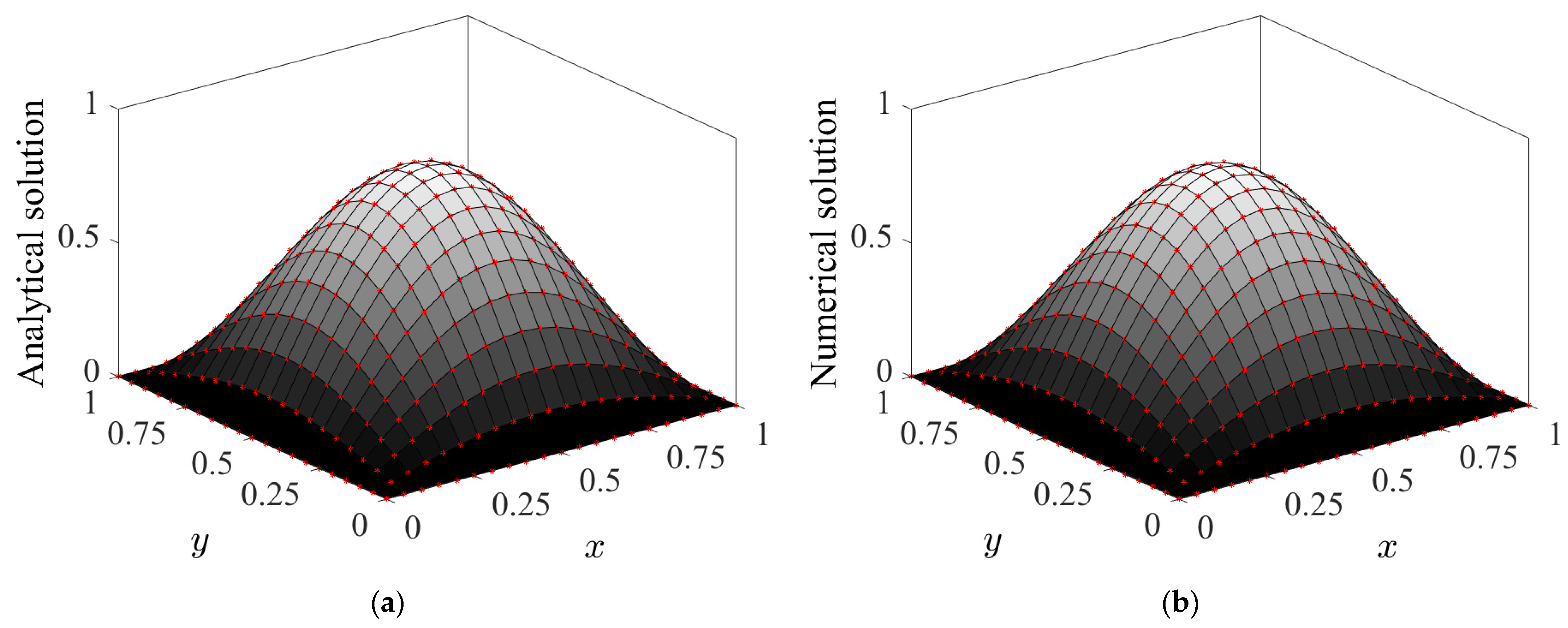
The p ^ ( x , y , z , t ) is described appropriately. We choose h = 0.1 ,   0.05 and Δ t = 0.01 . Table 2 shows the comparison between the proposed method and the existing ones in terms of RMS error norms. It can be noted that the present solutions are more accurate than the solutions presented in [16] by EFG and MLPG methods, and Expo-MCBDQM [17]. Figure 2 illustrates the absolute error norms for fixed z = 0.5 with h = 0.05 at t = 1 while Figure 3 shows the behavior of the solutions. From Figure 2 and Figure 3, one can notice that the absolute error norms are very small, and analytical and numerical solutions are very close each other which shows the accuracy of the proposed method.
Example 2.
Next, we consider Equation (1) for α 1 = δ = κ , α 2 = 0 and f ( u ) = u 2 with the analytical solution u ( x , y , z , t ) = sin π x   sin π y   sin π z   e κ t .
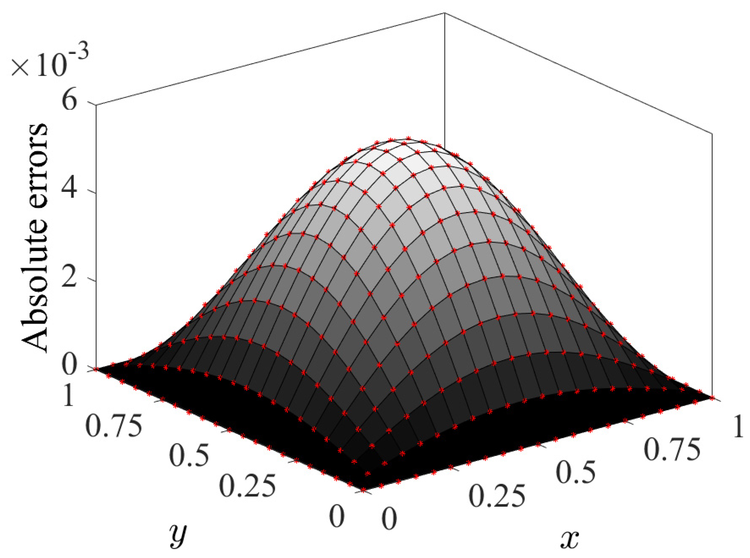
The function p ^ ( x , y , z , t ) is described appropriately and we choose the parameters h = 0.05, 0.1, Δ t = 0.01, and κ = 3 for the numerical approximation of this example. The proposed method is again compared with EFG [16] and MLPG [16] methods, and Expo-MCBDQM [17] in terms of RMS error norms and shown in Table 3. It is noticed that the proposed method shows better solutions than the solutions presented in [16,17]. Figure 4 illustrates the absolute error norms for z = 1, h = 0.05 at t = 1 while Figure 5 demonstrates the comparison of the analytical and numerical solutions, where a close agreement is noticed between analytical and numerical solutions. From Figure 4, one can notice that the absolute error norms are very small in 10−19, which shows that the proposed method provides very accurate results.
Example 3.
Finally, we consider Equation (1) for α 1 = α 2 = 0 , δ = 2 and f ( u ) = u with the analytical solution u ( x , y , z , t ) = sin π x   sin π y   sin π z   sin t .
The function p ^ ( x , y , z , t ) is chosen appropriately. We choose the parameters h = 0.05 and 0.1, Δ t = 0.01 . The present solutions are compared with the solutions obtained by EFG [16] and MLPG [16] methods, and Expo-MCBDQM [17] in terms of RMS error norms and shown in Table 4. Again, it is noticed that the proposed method provides better solutions than the existing methods. Figure 6 illustrates the absolute error norms for z = 0.5 , h = 0.05 at t = 1 . Figure 7 shows the comparison of the analytical and numerical solutions.

Computational Complexity

The system of equations, where the coefficient matrix is tridiagonal, is solved by using the Thomas algorithm which takes 3 M subtractions, 3 M multiplications, and 2 M + 1 divisions. Therefore, the algorithm needs a total of 8 M + 1 simple arithmetic operations. Therefore, the Thomas algorithm requires O ( n ) operations. The computational cost of the SSPRK-(5,4) technique is same as the cost of traditional ODE solvers. Hence, the proposed technique is not too complex from the computational point of view.

5. Conclusions

This work proposed a differential quadrature method based on cubic hyperbolic B-spline functions together with SSPRK-(5,4) scheme to solve 3D wave equations. The numerical examples show that the proposed method provides more accurate solutions than those discussed in [16,17]. The matrix stability analysis is also investigated, and we found that the proposed method is stable. Additionally, the method is economically easy-to-implement for solving hyperbolic partial differential equations. Moreover, the computational complexity shows that the proposed technique is not too complex from the computational point of view.

Author Contributions

Formal analysis, M.T.; investigation, M.T.; methodology, M.T.; validation, M.Z.M.; writing—original draft, M.T. and M.Z.M.; writing—review and editing, A.H.M. All authors have read and agreed to the published version of the manuscript.

Funding

This research received no external funding.

Data Availability Statement

Not applicable.

Conflicts of Interest

The authors declare no conflict of interest.

References

  1. Chen, H.; Zhou, H.; Jiang, S.; Rao, Y. Fractional Laplacian viscoacoustic wave equation low-rank temporal extrapolation. IEEE Access 2019, 99, 1–11. [Google Scholar] [CrossRef]
  2. Li, P.-W.; Fan, C.-M. Generalized finite difference method for two-dimensional shallow water equations. Eng. Anal. Bound. Elem. 2017, 80, 58–71. [Google Scholar] [CrossRef]
  3. Baccouch, M.; Temimi, H. A high-order space-time ultra-weak discontinuous Galerkin method for the second-order wave equation in one space dimension. J. Comput. Appl. Math. 2021, 389, 113331. [Google Scholar] [CrossRef]
  4. Yang, S.P.; Liu, F.W.; Feng, L.B.; Turner, I. A novel finite volume method for the nonlinear two-sided space distributed-order diffusion equation with variable coefficients. J. Comput. Appl. Math. 2021, 388, 113337. [Google Scholar] [CrossRef]
  5. Xie, X.; Liu, Y.J. An adaptive model order reduction method for boundary element-based multi-frequency acoustic wave problems. Comput. Meth. Appl. Mech. Engin. 2021, 373, 113532. [Google Scholar] [CrossRef]
  6. Takekawa, J.; Mikada, H. A mesh-free finite-difference method for elastic wave propagation in the frequency-domain. Comput. Geosci. 2018, 118, 65–78. [Google Scholar] [CrossRef]
  7. Gao, L.F.; Keyes, D. Combining finite element and finite difference methods for isotropic elastic wave simulations in an energy-conserving manner. J. Comput. Phys. 2019, 378, 665–685. [Google Scholar] [CrossRef] [Green Version]
  8. Ranocha, H.; Mitsotakis, D.; Ketcheson, D.I. A broad class of conservative numerical methods for dispersive wave equations. Commun. Comput. Phys. 2021, 29, 979–1029. [Google Scholar] [CrossRef]
  9. Wang, F.; Zhang, J.; Ahmad, I.; Farooq, A.; Ahmad, H. A novel meshfree strategy for a viscous wave equation with variable coefficients. Front. Phys. 2021, 9, 359. [Google Scholar]
  10. Bakushinsky, A.B.; Leonov, A.S. Numerical solution of a three-dimensional coefficient inverse problem for the wave equation with integral data in a cylindrical domain. Numer. Analys. Appl. 2019, 12, 311–325. [Google Scholar] [CrossRef]
  11. Dehghan, M. On the solution of an initial-boundary value problem that combines Neumann and integral condition for the wave equation. Numer. Meth. Part. Diff. Eq. 2005, 21, 24–40. [Google Scholar] [CrossRef]
  12. Dehghan, M. Finite difference procedures for solving a problem arising in modeling and design of certain optoelectronic devices. Math. Comput. Simul. 2006, 71, 16–30. [Google Scholar] [CrossRef]
  13. Mohanty, R.K.; Gopal, V. A new off-step high order approximation for the solution of three-space dimensional nonlinear wave equations. Appl. Math. Model. 2013, 37, 2802–2815. [Google Scholar] [CrossRef]
  14. Titarev, V.A.; Toro, E.F. ADER schemes for three-dimensional non-linear hyperbolic systems. J. Comput. Phys. 2005, 204, 715–736. [Google Scholar] [CrossRef]
  15. Zhang, Z.; Li, D.; Cheng, Y.; Liew, K. The improved element-free Galerkin method for three-dimensional wave equation. Acta Mech. Sin. 2012, 28, 808–818. [Google Scholar] [CrossRef]
  16. Shivanian, E. Meshless local Petrov-Galerkin (MLPG) method for three-dimensional nonlinear wave equations via moving least squares approximation. Eng. Anal. Bound. Elem. 2015, 50, 249–257. [Google Scholar] [CrossRef]
  17. Shukla, H.S.; Tamsir, M.; Jiwari, R.; Srivastava, V.K. A numerical algorithm for computation modelling of 3D nonlinear wave equations based on exponential modified cubic B-spline differential quadrature method. Int. J. Comput. Math. 2018, 95, 752–766. [Google Scholar] [CrossRef]
  18. Bellman, R.; Kashef, B.G.; Casti, J. Differential quadrature: A technique for the rapid solution of nonlinear differential equations. J. Comput. Phy. 1972, 10, 40–52. [Google Scholar] [CrossRef]
  19. Korkmaz, A.; Dag, I. Shock wave simulations using sinc differential quadrature method. Eng. Comput. 2011, 28, 654–674. [Google Scholar] [CrossRef]
  20. Shu, C.; Chew, Y.T. Fourier expansion-based differential quadrature and its application to Helmholtz eigenvalue problems. Commun. Numer. Methods Eng. 1997, 13, 643–653. [Google Scholar] [CrossRef]
  21. Shu, C.; Xue, H. Explicit computation of weighting coefficients in the harmonic differential quadrature. J. Sound Vib. 1997, 204, 549–555. [Google Scholar] [CrossRef]
  22. Bashan, A.; Karakoc, S.B.G.; Geyikli, T. Approximation of the KdVB equation by the quintic B-spline differential quadrature method. Kuwait J. Sci. 2015, 42, 67–92. [Google Scholar]
  23. Korkmaz, A.; Dag, I. Cubic B-spline differential quadrature methods and stability for Burgers equation. Eng. Comput. 2013, 30, 320–344. [Google Scholar] [CrossRef]
  24. Shukla, H.S.; Tamsir, M.; Srivastava, V.K.; Kumar, J. Numerical solution of two dimensional coupled viscous Burger equation using modified cubic B-spline differential quadrature method. AIP Adv. 2014, 4, 117134. [Google Scholar] [CrossRef]
  25. Shukla, H.S.; Tamsir, M.; Srivastava, V.K. Numerical simulation of two dimensional sine-Gordon solitons using modified cubic B-spline differential quadrature method. AIP Adv. 2015, 5, 017121. [Google Scholar] [CrossRef]
  26. Korkmaz, A.; Dag, I. Cubic B-spline differential quadrature methods for the advection-diffusion equation. Int. J. Numer. Meth. Heat Fluid Flow 2012, 22, 1021–1036. [Google Scholar] [CrossRef]
  27. Tamsir, M.; Srivastava, V.K.; Jiwari, R. An algorithm based on exponential modified cubic B-spline differential quadrature method for nonlinear Burgers’ equation. Appl. Math. Comput. 2016, 290, 111–124. [Google Scholar] [CrossRef]
  28. Jiwari, R.; Pandit, S.; Mittal, R.C. Numerical simulation of two-dimensional sine-Gordon solitons by differential quadrature method. Comput. Phys. Commun. 2012, 183, 600–616. [Google Scholar] [CrossRef]
  29. Korkmaz, A.; Dag, I. Numerical simulations of boundary-forced RLW equation with cubic B-spline-based differential quadrature methods. Arab. J. Sci. Eng. 2013, 38, 1151–1160. [Google Scholar] [CrossRef]
  30. Korkmaz, A.; Dag, I. Quartic and quintic B-spline methods for advection diffusion equation. Appl. Math. Comput. 2016, 274, 208–219. [Google Scholar] [CrossRef]
  31. Jiwari, R. Lagrange interpolation and modified cubic B-spline differential quadrature methods for solving hyperbolic partial differential equations with Dirichlet and Neumann boundary conditions. Comput. Phys. Commun. 2015, 193, 55–65. [Google Scholar] [CrossRef]
  32. Lin, J.; Reutskiy, S. A cubic B-spline semi-analytical algorithm for simulation of 3D steady-state convection-diffusion-reaction problems. Appl. Math. Comput. 2020, 371, 124944. [Google Scholar] [CrossRef]
  33. Ali, I.; Seadawy, A.R.; Rizvi, S.T.R.; Younis, M.; Ali, K. Conserved quantities along with Painlevé analysis and optical solitons for the nonlinear dynamics of Heisenberg ferromagnetic spin chains model. Int. J. Mod. Phys. B 2020, 34, 2050283. [Google Scholar] [CrossRef]
  34. Lu, D.; Seadwy, A.R.; Iqbal, M. Mathematical methods via construction of traveling and solitary wave solutions of three coupled system of nonlinear partial differential equations and their applications. Res. Phys. 2018, 11, 1161–1171. [Google Scholar] [CrossRef]
  35. Seadawy, A.R.; Khalid, K.A.; Nuruddeen, R.I. A variety of soliton solutions for the fractional Wazwaz-Benjamin-Bona-Mahony equations. Res. Phys. 2019, 12, 2234–2241. [Google Scholar]
  36. Akram, U.; Seadawy, A.R.; Rizvi, S.T.R.; Younis, M.; Althobaiti, S.; Sayed, S. Traveling wave solutions for the fractional Wazwaz–Benjamin–Bona–Mahony model in arising shallow water waves. Res. Phys. 2021, 20, 103725. [Google Scholar] [CrossRef]
  37. Ahlberg, J.H.; Nilson, E.N.; Walsh, J.L. The Theory of Splines and Their Applications; Academic Press: New York, NY, USA, 1967. [Google Scholar]
  38. Lu, C. Error analysis for interpolating complex cubic splines with deficiency 2. J. Approx. Theory 1982, 36, 183–196. [Google Scholar] [CrossRef] [Green Version]
  39. Kapoor, M.; Joshi, V. Numerical approximation of 1D and 2D non-linear Schrödinger equations by implementing modified cubic Hyperbolic B-spline based DQM. Part. Diff. Eq. Appl. Math. 2021, 4, 100076. [Google Scholar] [CrossRef]
  40. Shu, C. Differential Quadrature and its Application in Engineering, 1st ed.; Athenaeum Press Ltd.: Newcastle Upon Tyne, UK, 2000. [Google Scholar]
  41. Gottlieb, S.; Ketcheson, D.I.; Shu, C.W. High order strong stability preserving time discretizations. J. Sci. Comput. 2009, 38, 251–289. [Google Scholar] [CrossRef]
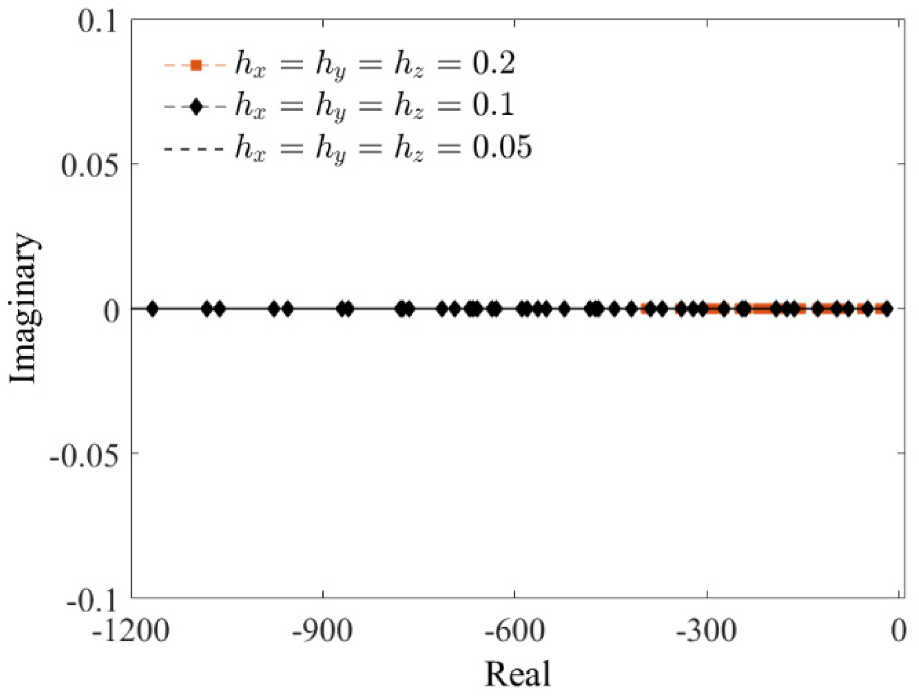
Figure 1. Eigenvalues of the matrix F 1 .
Axioms 11 00597 g001
Figure 2. The absolute error norms with h = 0.05 and Δ t = 0.01 for z = 0.5 at t = 1 .
Axioms 11 00597 g002
Figure 3. The analytical (a) and numerical (b) solutions with h = 0.05 and Δ t = 0.01 for z = 0.5 at t = 1 .
Axioms 11 00597 g003
Figure 4. The absolute error norms with h = 0.05 and Δ t = 0.01 for z = 1 at t = 1 .
Axioms 11 00597 g004
Figure 5. The analytical (a) and numerical (b) solutions with h = 0.05 and Δ t = 0.01 for z = 1 at t = 1 .
Axioms 11 00597 g005
Figure 6. The absolute error norms with h = 0.05 and Δ t = 0.01 for z = 0.5 at t = 1 .
Axioms 11 00597 g006
Figure 7. The numerical (a) and analytical (b) solutions with h = 0.05 and Δ t = 0.01 for z = 0.5 at t = 1 .
Axioms 11 00597 g007
Table 1. The values of cubic hyperbolic B-spline functions at the knots.
x i 2 x i 1 x i x i + 1 x i + 2
H f i ( x ) 0 ϒ 1 ϒ 2 ϒ 3 0
H f i ( x ) 0 ϒ 4 0 ϒ 5 0
Table 2. Comparison between the present method and existing methods with h = 0.1 and Δ t = 0.01 at different values of t for Example 1.
t Present MethodEFG Method [16]MLPG Method [16]Expo-MCBDQM [17]
0.19.131 × 10−71.361376 × 10−16.389040 × 10−41.013 × 10⁻⁶
0.29.126 × 10−71.108673 × 10−11.621007 × 10−31.666 × 10⁻⁶
0.39.751 × 10−79.031794 × 10−22.069397 × 10−31.725 × 10⁻⁶
0.49.357 × 10−77.555177 × 10−21.851491 × 10−31.498 × 10⁻⁶
0.59.263 × 10−76.113317 × 10−21.406413 × 10−31.196 × 10⁻⁶
0.68.105 × 10−75.076050 × 10−21.120239 × 10−39.059 × 10⁻⁷
0.76.102 × 10−74.276296 × 10−28.762877 × 10−47.061 × 10⁻⁷
0.84.458 × 10−73.416178 × 10−25.762842 × 10−45.566 × 10⁻⁷
0.93.614 × 10−73.072394 × 10−27.778958 × 10−44.758 × 10⁻⁷
1.03.326 × 10−72.562088 × 10−28.638225 × 10−44.417 × 10⁻⁷
Table 3. Comparison between the present method and existing methods with h = 0.1 and Δ t = 0.01 at different values of t for Example 2.
t Present MethodEFG Method [16]MLPG Method [17]Expo-MCBDQM [17]
0.14.472 × 10−61.653265 × 1002.777931 × 10−35.667 × 10⁻⁶
0.28.511 × 10−61.005632 × 1008.477482 × 10−39.701 × 10⁻⁶
0.32.23 × 10−69.786343 × 10−11.352534 × 10−21.231 × 10⁻⁵
0.45.02 × 10−67.456237 × 10−11.583307 × 10−21.512 × 10⁻⁵
0.51.143 × 10−56.213675 × 10−11.550351 × 10−21.824 × 10⁻⁵
0.61.062 × 10−54.354421 × 10−11.367202 × 10−22.222 × 10⁻⁵
0.71.231 × 10−51.345213 × 10−11.052578 × 10−22.570 × 10⁻⁵
0.81.324 × 10−59.973233 × 10−26.216680 × 10−32.866 × 10⁻⁵
0.92.014 × 10−57.132423 × 10−25.280951 × 10−33.117 × 10⁻⁵
1.02.1025 × 10−56.124572 × 10−22.276681 × 10−33.329 × 10⁻⁵
Table 4. Comparison between the present method and existing methods with h = 0.1 and Δ t = 0.01 at different values of t for Example 3.
t Present MethodEFG Method [16]MLPG Method [16]Expo-MCBDQM [17]
0.11.673 × 10−71.435666 × 10−38.903029 × 10−52.887 × 10⁻⁷
0.22.481 × 10−73.867576 × 10−39.910264 × 10−51.257 × 10⁻⁶
0.31.522 × 10−65.033494 × 10−31.590358 × 10−42.944 × 10⁻⁶
0.44.137 × 10−67.655177 × 10−33.776687 × 10−45.348 × 10⁻⁶
0.57.465 × 10−69.119769 × 10−34.781290 × 10−48.787 × 10⁻⁶
0.63.304 × 10−61.034540 × 10−26.416380 × 10−41.361 × 10⁻⁵
0.71.007 × 10−53.279875 × 10−28.809498 × 10−42.029 × 10⁻⁵
0.81.716 × 10−55.233178 × 10−29.279331 × 10−42.918 × 10⁻⁵
0.93.014 × 10−56.072234 × 10−21.059260 × 10−44.049 × 10⁻⁵
1.04.221 × 10−57.545088 × 10−21.529316 × 10−35.432 × 10⁻⁵
Publisher’s Note: MDPI stays neutral with regard to jurisdictional claims in published maps and institutional affiliations.