
Testing Multivariate Normality Based on t-Representative Points

Abstract
1. Introduction
2. A Brief Review on the MVN Characterization
- 1.
- are mutually independent and () has a symmetric multivariate Pearson Type II distribution with a p.d.f.,
- 2.
- are mutually independent and () has a symmetric multivariate Pearson Type VII distribution with a p.d.f.,
- 3.
- Let be i.i.d. in with a p.d.f. , which is continuous in and . Define the random vectors by (1). If and () have p.d.f.’s and defined by (3), respectively, then () has a multivariate normal distribution.
3. The RP-Based Chi-Square Test
4. A Monte Carlo Study and an Illustrative Example
4.1. A Comparison between Empirical Type I Error Rates
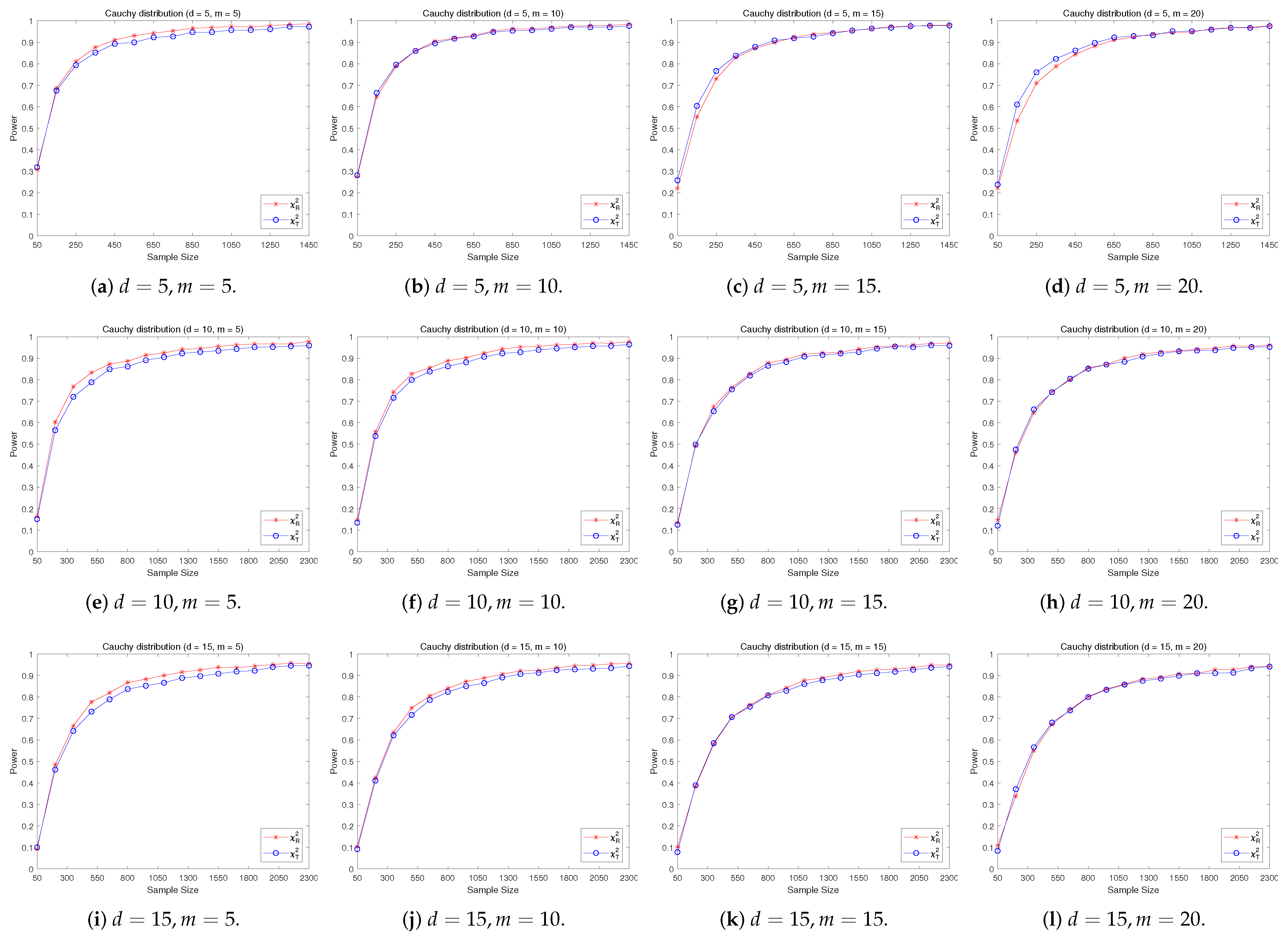
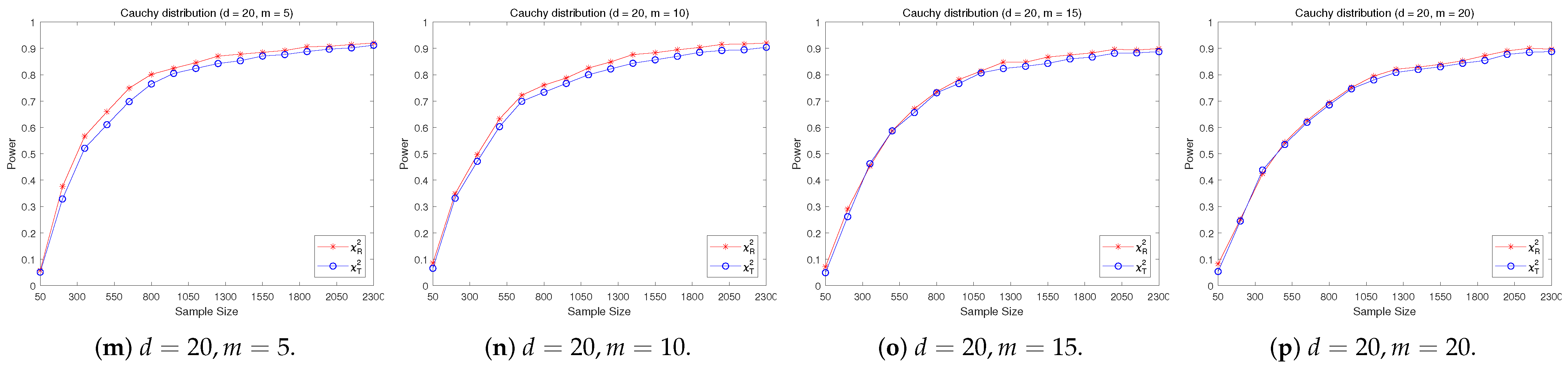
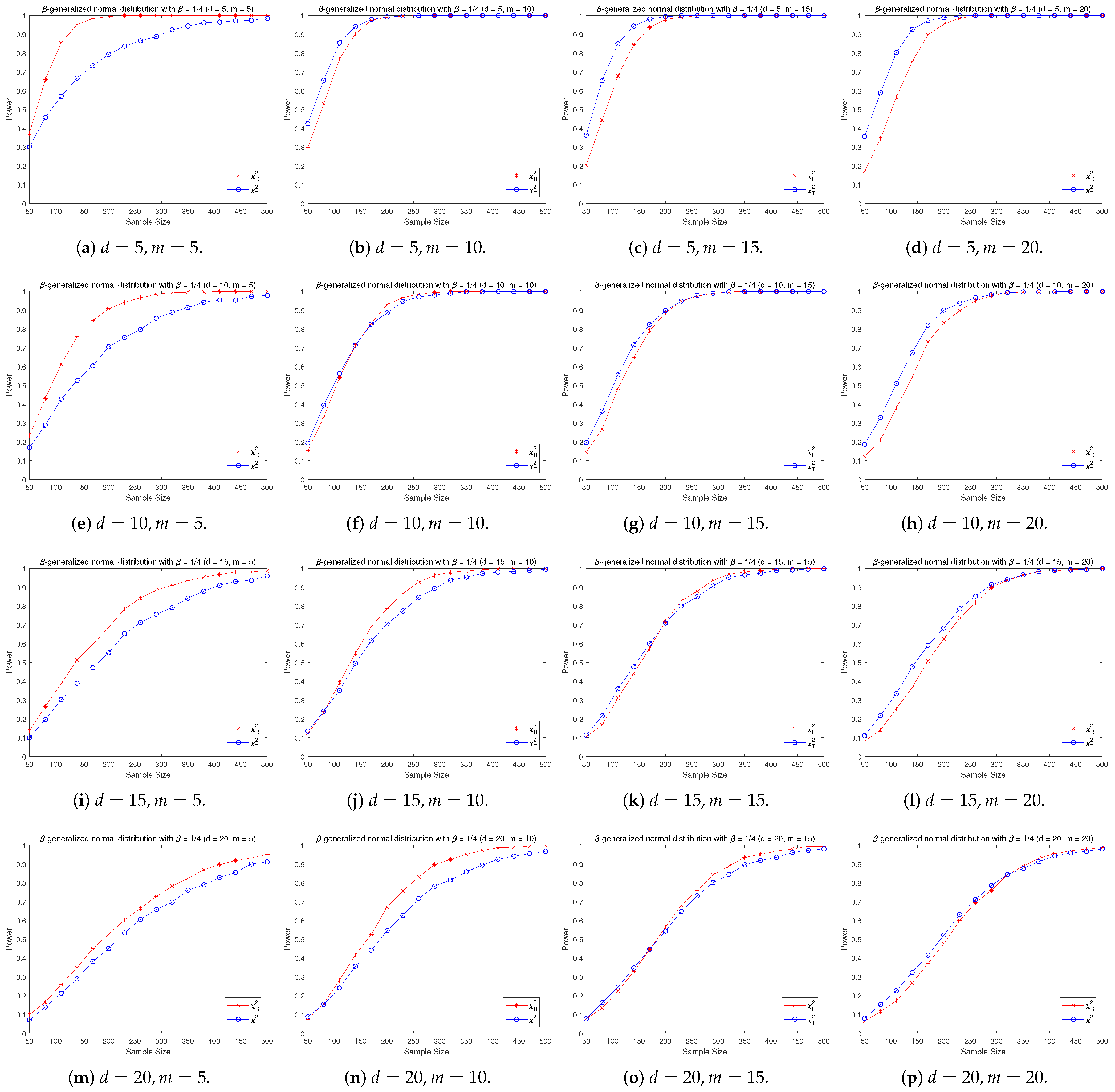
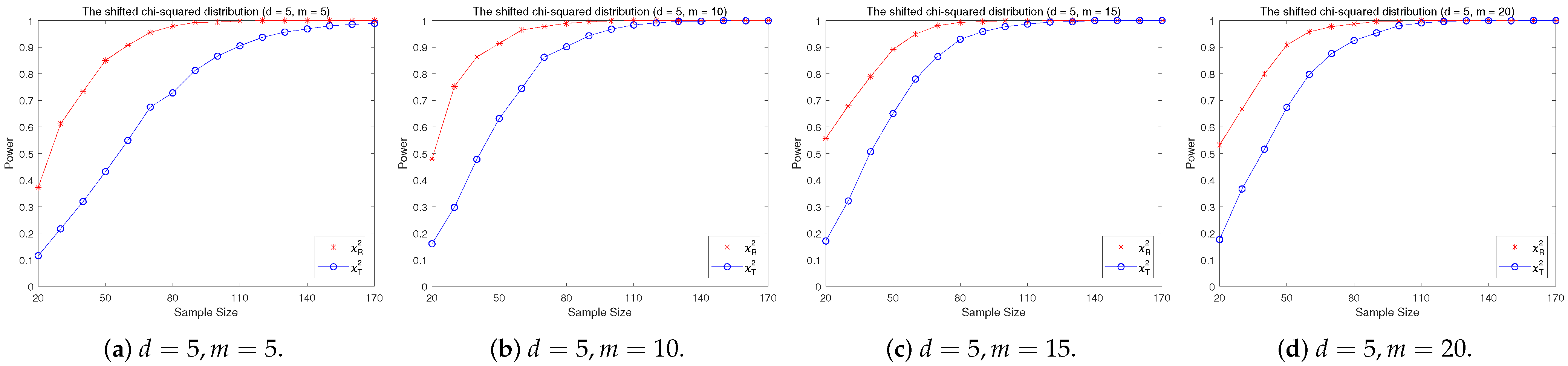
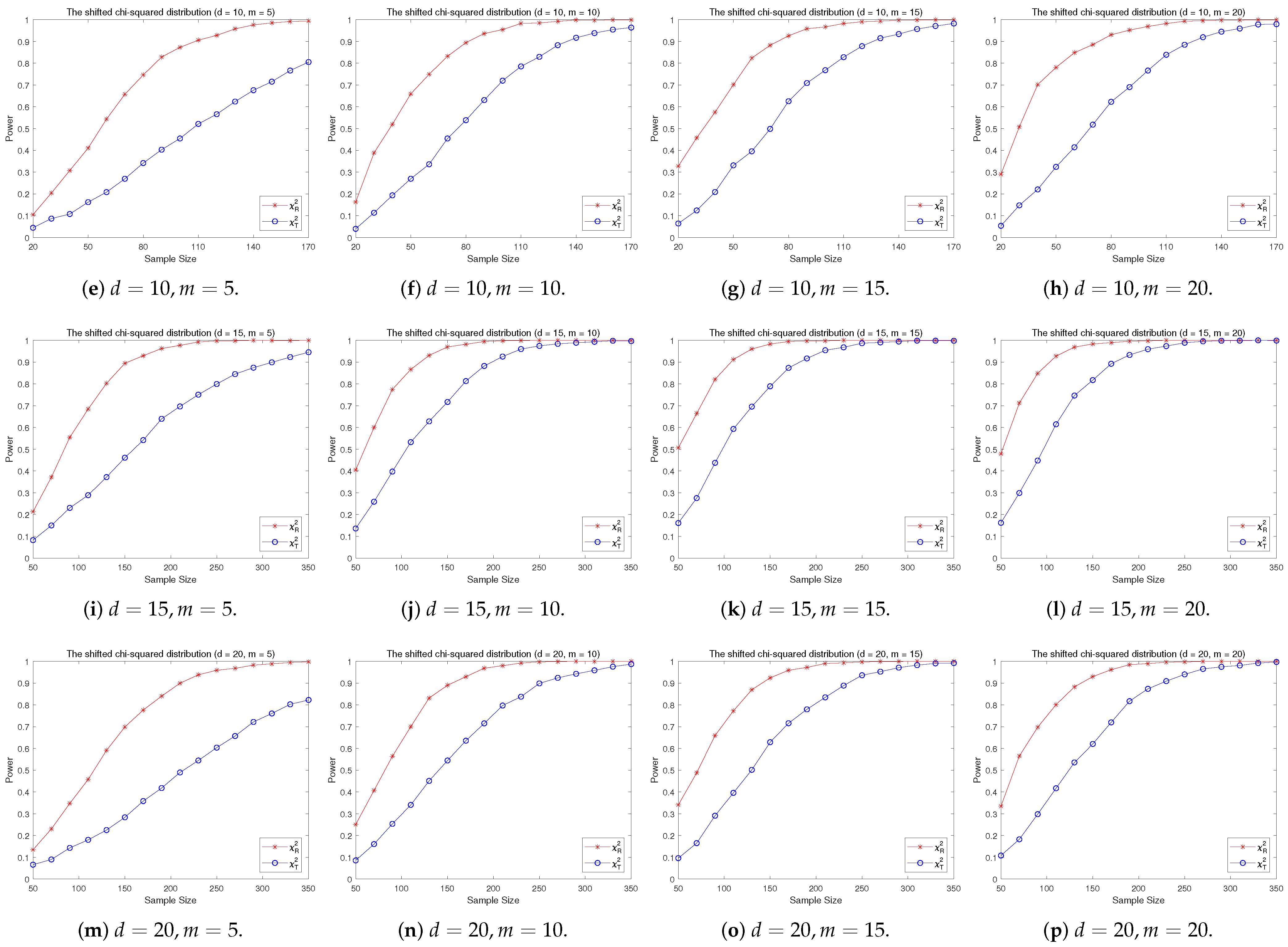
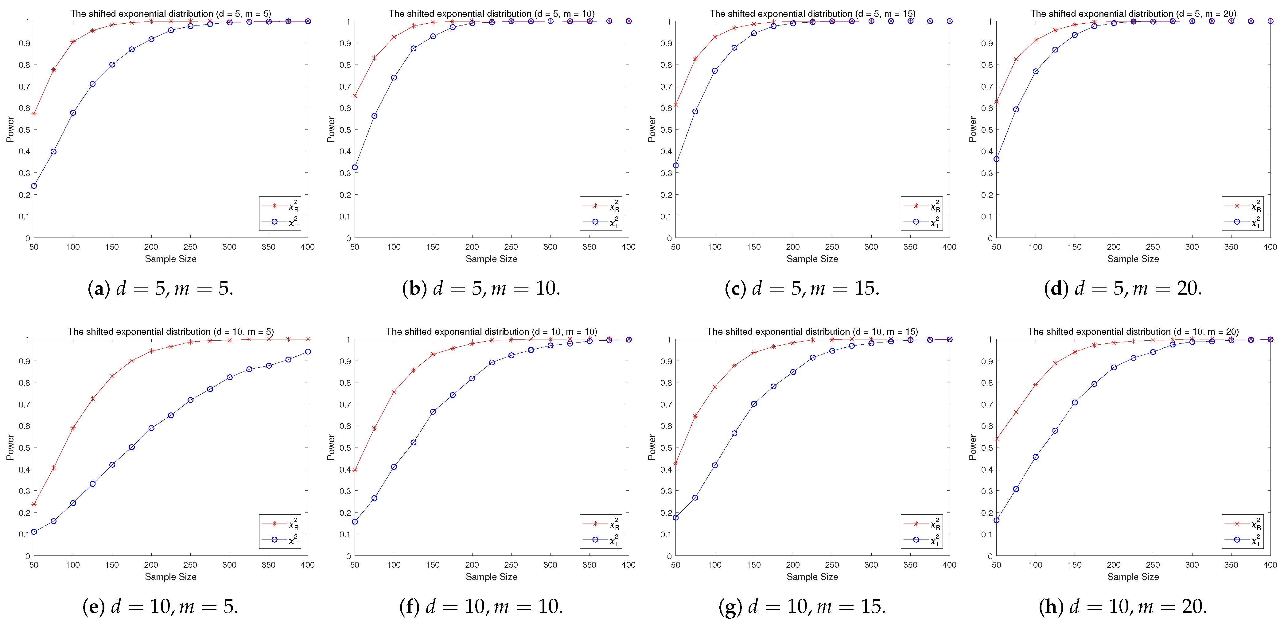
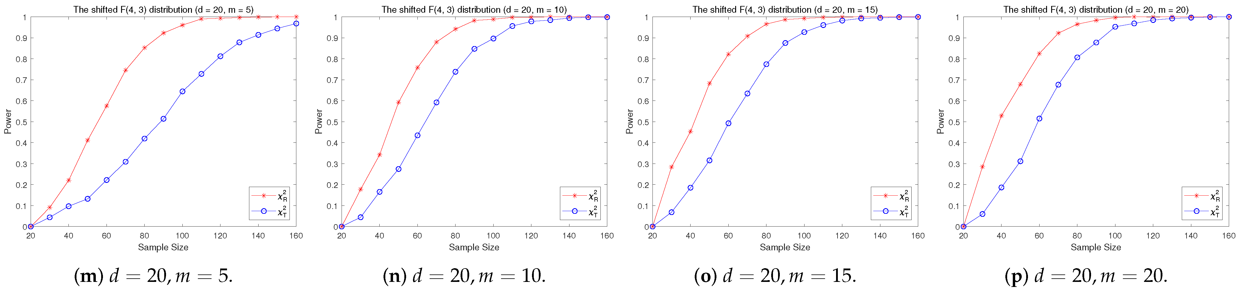
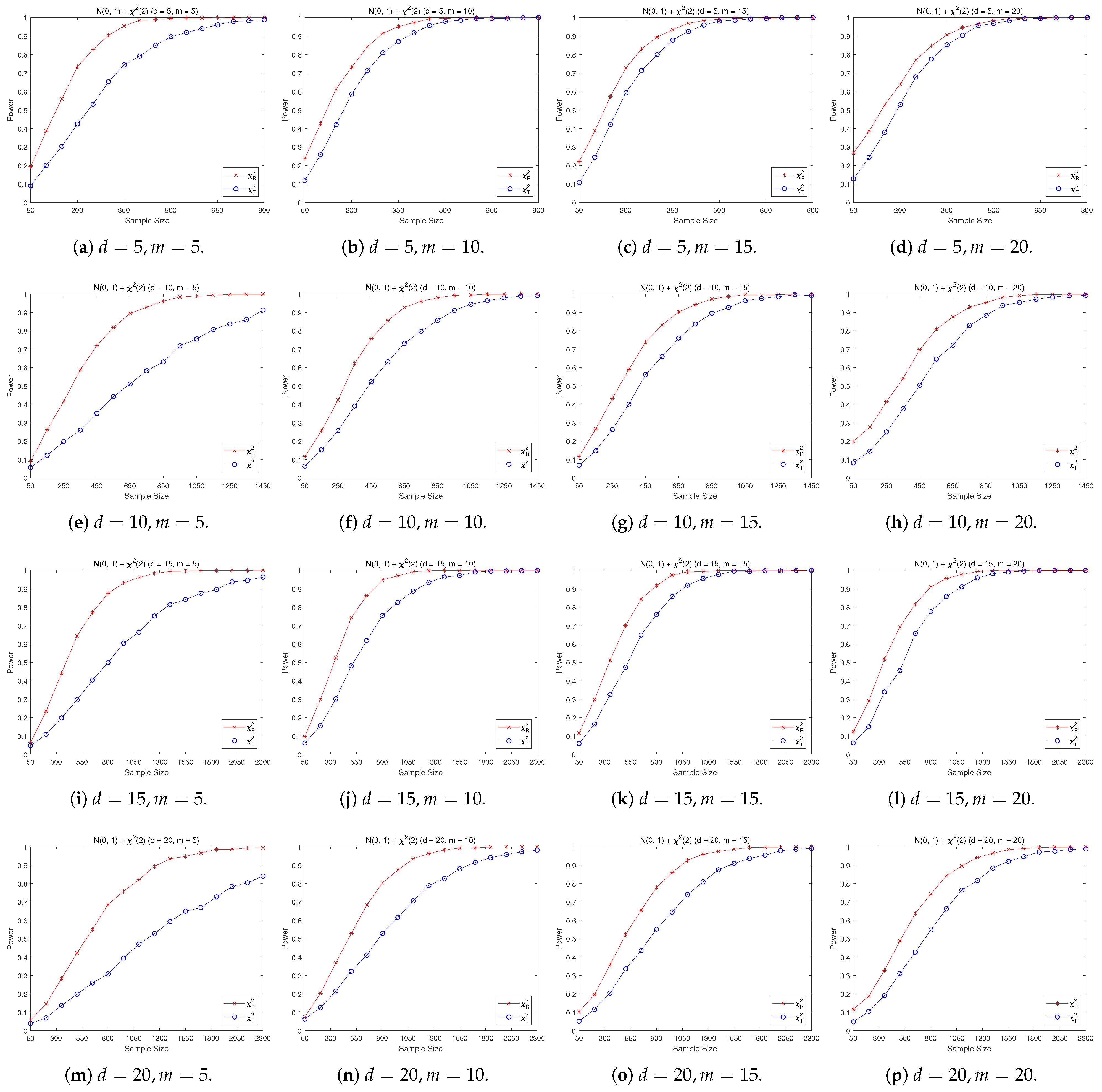
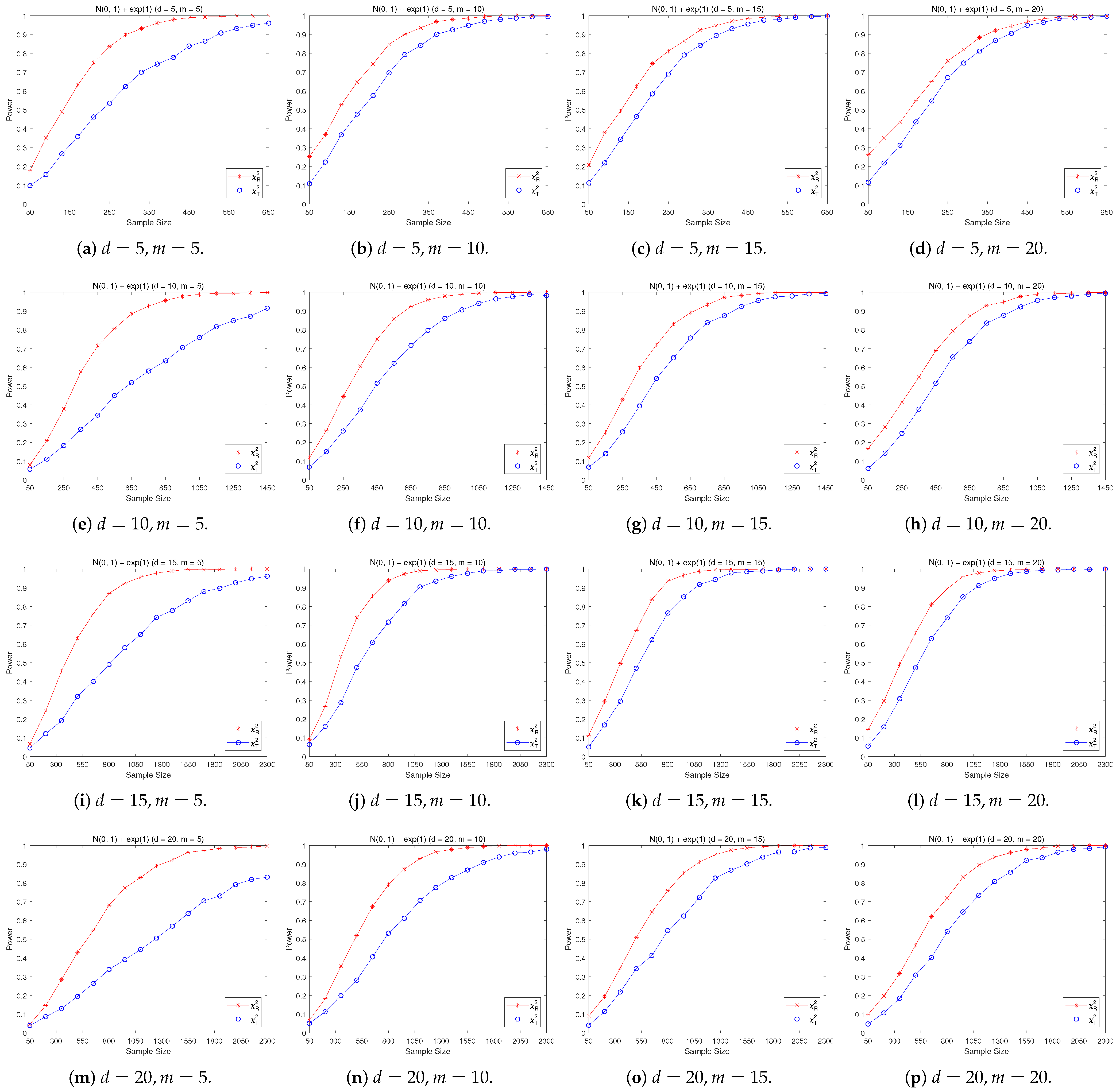
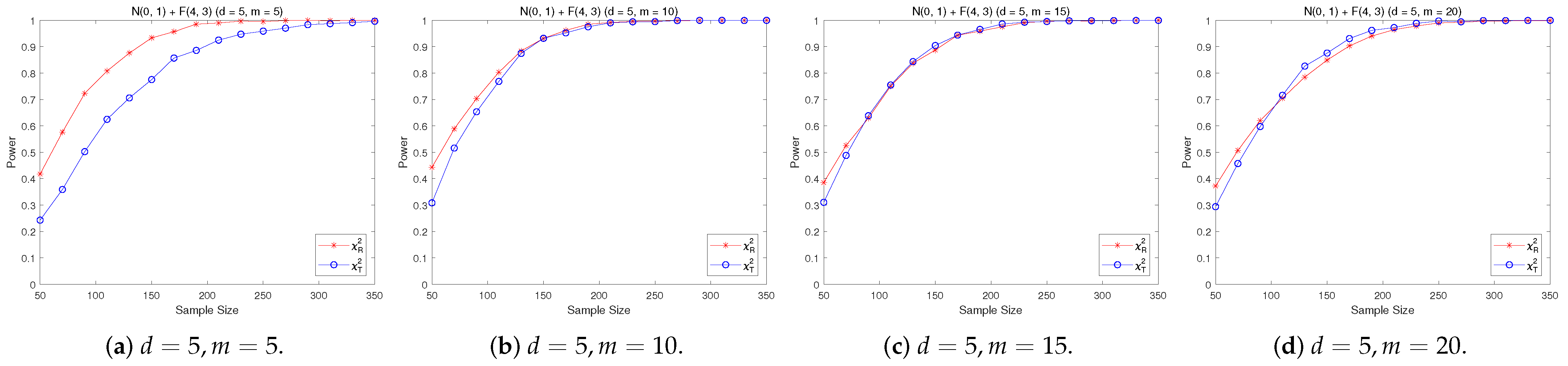
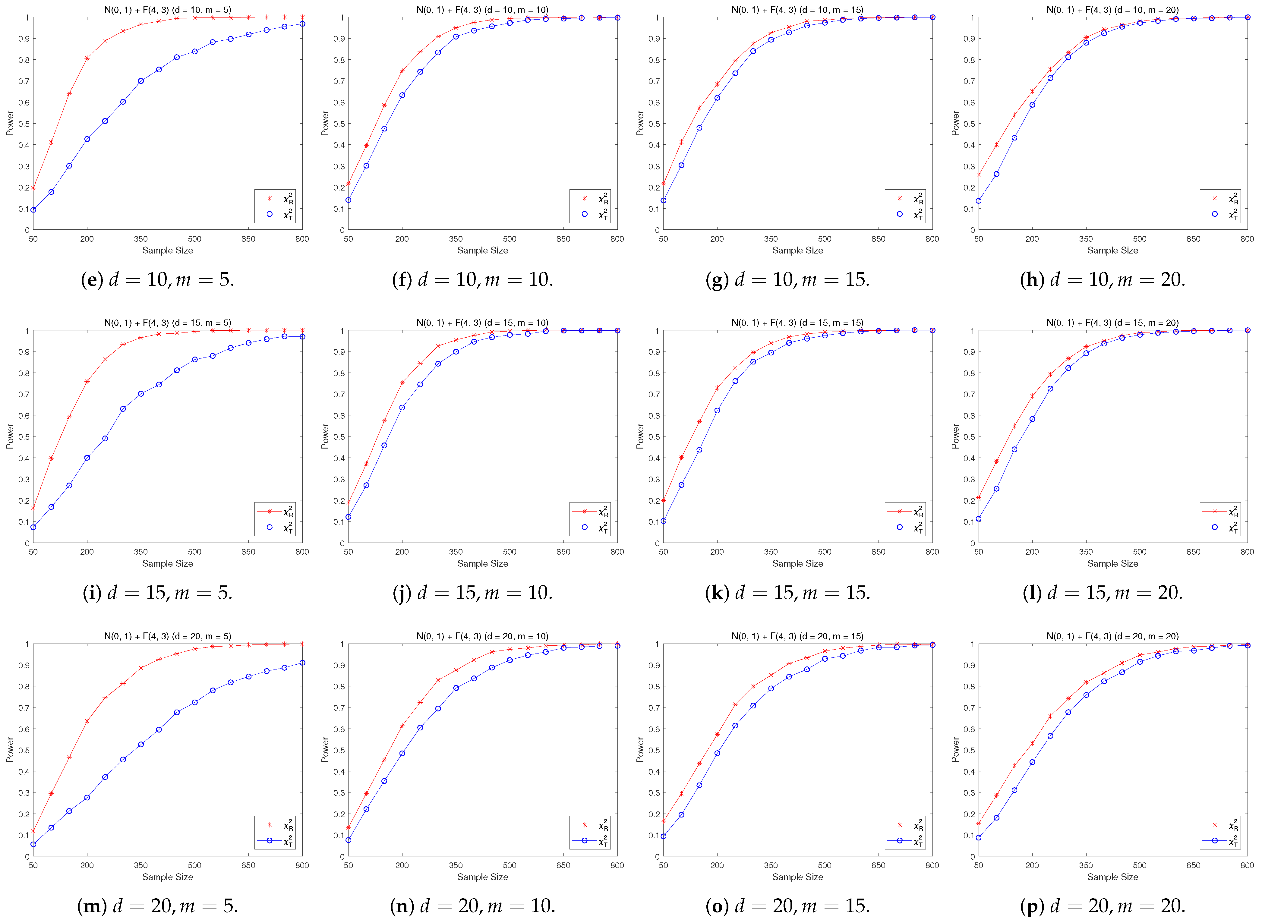
4.2. A Simple Power Comparison
- (1)
- [symmetric] The multivariate Cauchy distribution ([22]) has a density function of the form:where “” stands for the Euclidean norm of a vector, is a normalizing constant depending on the dimension d.
- (2)
- [symmetric] The -generalized normal distribution with has a density function of the form by ([28]):where is a parameter. Let in the simulation and denote it by -normal.
- (3)
- [symmetric] Multivariate double Weibull distribution consisting of i.i.d. univariate double Weibull distributions ([29]), its density function is given by:where and are the shape parameter and scale parameter, respectively. Let and in the simulation.
- (4)
- [skewed] The shifted i.i.d. with i.i.d. marginals, each marginal has the same distribution as that of the random variable , where , the univariate chi-square distribution with 1 degree of freedom and .
- (5)
- [skewed] The shifted i.i.d. with i.i.d. marginals, each marginal has the same distribution as that of the random variable , where , the univariate exponential distribution.
- (6)
- [skewed] The shifted i.i.d. F-distribution with i.i.d. marginals with i.i.d. marginals, , where , .
- (7)
- [A distribution with normal marginals] The distribution consists of i.i.d. normal marginals and i.i.d. marginals, where stands for the integer part of .
- (8)
- [A distribution with normal marginals] The distribution consists of i.i.d. normal marginals and i.i.d. marginals.
- (9)
- [A distribution with normal marginals] The distribution consists of i.i.d. normal marginals and i.i.d. marginals.
- (1)
- The RP chi-square test is comparable to (or slightly better than) the traditional test for symmetric alternative distributions;
- (2)
- The RP chi-square test is able to improve the traditional test significantly for both skewed and normal+skewed alternative distributions.
4.3. An Illustrative Example
- (1)
- The 5-dimensional random vector can be approximately considered as 5-dimensional normal;
- (2)
- The 5-dimensional random vector shows evidence of non-MVN;
- (3)
- The 5-dimensional random vector shows evidence of non-MVN;
- (4)
- The 5-dimensional random vector shows evidence of non-MVN;
- (5)
- The 10-dimensional random vector shows evidence of non-MVN;
- (6)
- The 10-dimensional random vector can be approximately considered as 10-dimensional normal;
- (7)
- The 10-dimensional random vector shows evidence of non-MVN;
- (8)
- The 10-dimensional random vector can be approximately considered as 10-dimensional normal.
- (1)
- The 5-dimensional random vector can be approximately considered as 5-dimensional normal by for and , and by for ;
- (2)
- The 5-dimensional random vector shows evidence of non-MVN by for . fails to detect the non-MVN for all three choices of m;
- (3)
- The 5-dimensional random vector shows evidence of non-MVN by both and for all three choices of m;
- (4)
- The 5-dimensional random vector shows evidence of non-MVN by for and , and by for and ;
- (5)
- The 10-dimensional random vector shows evidence of non-MVN by for . fails to detect the non-MVN for all three choices of m;
- (6)
- The 10-dimensional random vector shows evidence of non-MVN by for and . fails to detect the non-MVN for all three choices of m;
- (7)
- The 10-dimensional random vector can be approximately considered as 10-dimensional normal by both and for all three choices of m;
- (8)
- The 10-dimensional random vector can be approximately considered as 10-dimensional normal by both and .
5. Concluding Remarks
Author Contributions
Funding
Data Availability Statement
Conflicts of Interest
Abbreviations
| i.i.d. | Independent identically distributed |
| MVN | Multivariate normality |
| p.d.f. | Probability density function |
| RP | Representative points |
References
- Anderson, M.R. A characterization of the multivariate normal distribution. Ann. Math. Stat. 1971, 42, 824–827. [Google Scholar] [CrossRef]
- Shao, Y.; Zhou, M. A characterization of multivariate normality through univariate projections. J. Multivar. Anal. 2010, 101, 2637–2640. [Google Scholar] [CrossRef] [PubMed]
- Malkovich, J.F.; Afifi, A.A. On tests for multivariate normality. J. Am. Stat. Assoc. 1973, 68, 176–179. [Google Scholar] [CrossRef]
- Cox, D.R.; Small, N.J.H. Testing multivariate normality. Biometrika 1978, 65, 263–272. [Google Scholar] [CrossRef]
- Andrews, D.F.; Gnanadesikan, R.; Warner, J.L. Methods for assessing multivariate normality. In Proceedings of the Third International Symposium on Multivariate Analysis, Dayton, OH, USA, 19–24 June 1972; Volume 3, pp. 95–116. [Google Scholar]
- Gnanadesikan, R. Methods for Statistical Data Analysis of Multivariate Observations; Wiley: New York, NY, USA, 1977. [Google Scholar]
- Mardia, K.V. Measures of multivariate skewness and kurtosis with applications. Biometrika 1970, 57, 519–530. [Google Scholar] [CrossRef]
- Mardia, K.V. Tests of univariate and multivariate normality. In Handbook of Statistics; Krishnaiah, P.R., Ed.; North-Holland Publishing Company: Amsterdam, The Netherlands, 1980; Volume 1, pp. 279–320. [Google Scholar]
- Romeu, J.L.; Ozturk, A. A comparative study of goodness-of-fit tests for multivariate normality. J. Multivar. Anal. 1993, 46, 309–334. [Google Scholar] [CrossRef]
- Horswell, R.L.; Looney, S.W. A comparison of tests for multivariate normality that are based on measures of multivariate skewness and kurtosis. J. Stat. Comput. Simul. 1992, 42, 21–38. [Google Scholar] [CrossRef]
- Looney, S.W. How to use tests for univariate normality to assess multivariate normality. Am. Stat. 1995, 39, 75–79. [Google Scholar]
- Liang, J.; Li, R.; Fang, H.; Fang, K.T. Testing multinormality based on low-dimensional projection. J. Stat. Plann. Infer. 2000, 86, 129–141. [Google Scholar] [CrossRef]
- Srivastava, D.K.; Mudholkar, G.S. Goodness-of-fit tests for univariate and multivariate normal models. Handb. Stat. 2003, 22, 869–906. [Google Scholar]
- Mecklin, C.J.; Mundfrom, D.J. An appraisal and bibliography of tests for multivariate normality. Int. Stat. Rev. 2004, 72, 123–138. [Google Scholar] [CrossRef]
- Batsidis, A.; Martin, N.; Pardo, L.; Zografos, K. A Necessary power divergence type family tests of multivariate normality. Commun. Stat. Simul. Comput. 2013, 42, 2253–2271. [Google Scholar] [CrossRef]
- Al-Labadi, L.; Fazeli Asl, F.; Saberi, Z. A necessary Bayesian nonparametric test for assessing multivariate normality. Math. Methods Stat. 2021, 30, 64–81. [Google Scholar] [CrossRef]
- Doomik, J.A.; Hansen, H. An omnibus test for univariate and multivariate normality. Oxf. Bull. Econ. Stat. 2008, 70, 927–939. [Google Scholar]
- Ebner, B.; Henze, N. Tests for multivariate normality? a critical review with emphasis on weighted L2-statistics. Test 2020, 29, 845–892. [Google Scholar] [CrossRef]
- Yang, Z.H.; Fang, K.T.; Liang, J. A characterization of multivariate normal distribution and its application. Stat. Prob. Lett. 1996, 30, 347–352. [Google Scholar] [CrossRef]
- Liang, J.; Pan, W.; Yang, Z.H. Characterization-based Q-Q plots for testing multinormality. Stat. Prob. Lett. 2004, 70, 183–190. [Google Scholar] [CrossRef]
- Fang, K.T.; He, S.D. The Problem of Selecting a Given Number of Representative Points in a Normal Distribution and a Generalized Mill’s Ratio; Technical Report; Department of Statistics, Stanford University: Stanford, CA, USA, 1982. [Google Scholar]
- Fang, K.T.; Kotz, S.; Ng, K.W. Symmetric Multivariate and Related Distributions; Chapman and Hall: London, UK; New York, NY, USA, 1990. [Google Scholar]
- Pearson, K. On the criterion that a given system of deviations from the probable in the case of a correlated system of variables is such that it can be reasonably supposed to have arisen from random sampling. Philos. Mag. 1900, 50, 157–175. [Google Scholar] [CrossRef]
- Fisher, R.A. The condition under which χ2 measures the discrepancy between observation and hypothesis. J. R. Stat. Soc. 1924, 87, 442–450. [Google Scholar]
- Voinov, V.; Pya, N.; Alloyarova, R. A comparative study of some modified chi-squared tests. Commun. Stat. Simul. Comput. 2009, 38, 355–367. [Google Scholar] [CrossRef]
- Flury, B. Principal points. Biometrika 1990, 77, 33–41. [Google Scholar] [CrossRef]
- Zhou, M.; Wang, W. Representative points of the Student’s tn distribution and their applications in statistical simulation. Acta Math. Appl. Sin. 2016, 39, 620–640. (In Chinese) [Google Scholar]
- Goodman, I.R.; Kotz, S. Multivariate θ-generalized normal distribution. J. Multivar. Anal. 1973, 3, 204–219. [Google Scholar] [CrossRef]
- Perveen, Z.; Munir, M.; Ahmad, M. Double Weibull distribution: Properties and application. Pak. J. Sci. 2017, 69, 95–100. [Google Scholar]
- Liang, J.; Bentler, P.M. A t-distribution plot to detect non-multinormality. Comput. Stat. Data Anal. 1999, 30, 31–44. [Google Scholar] [CrossRef]
- Koehler, K.; Gann, F. Chi-squared goodness-of-fit tests: Cell Selection and Power. J. Commun. Stat. Simul. 1990, 19, 1265–1278. [Google Scholar] [CrossRef]
- Graf, S.; Luschgy, H. Foundations of Quantization for Probability Distributions; Springer: Berlin, Germany, 2000. [Google Scholar]
- Mann, H.; Wald, A. On the choice of the number of class intervals in the application of the chi-square test. Ann. Math. Stat. 1942, 13, 306–317. [Google Scholar] [CrossRef]
- Dahiya, R.C.; Gurland, J. How many classes in the Pearson chi-square test? J. Am. Stat. Assoc. 1973, 68, 707–712. [Google Scholar]
- Kallenberg, W.; Oosterhoff, J.; Schriever, B. The number of classes in chi-squared goodness-of-fit tests. J. Am. Stat. Assoc. 1985, 80, 959–968. [Google Scholar] [CrossRef]
- Korkmaz, S.; Goksuluk, D.; Zararsiz, G. MVN: An R package for assessing multivariate normality. R J. 2014, 6, 151–162. [Google Scholar] [CrossRef]
- Chernoff, H.; Lehmann, E.L. The use of maximum likelihood estimates in tests for goodness of fit. Ann. Math. Stat. 1954, 25, 579–589. [Google Scholar] [CrossRef]
- Voinov, V.; Nikulin, M.; Balakrishnan, N. Chi-Squared Goodness of Fit Tests with Applications; Academic Press: New York, NY, USA, 2013. [Google Scholar]


| n | m | |||||
|---|---|---|---|---|---|---|
| 0.0155 | 0.0110 | 0.0075 | 0.0070 | |||
| 0.0075 | 0.0070 | 0.0065 | 0.0075 | |||
| 0.0320 | 0.0145 | 0.0120 | 0.0125 | |||
| 0.0090 | 0.0105 | 0.0075 | 0.0085 | |||
| 0.0525 | 0.0285 | 0.0210 | 0.0235 | |||
| 0.0080 | 0.0105 | 0.0115 | 0.0090 | |||
| 0.0835 | 0.0465 | 0.0255 | 0.0340 | |||
| 0.0115 | 0.0110 | 0.0090 | 0.0130 | |||
| 0.0130 | 0.0100 | 0.0120 | 0.0105 | |||
| 0.0070 | 0.0125 | 0.0105 | 0.0150 | |||
| 0.0350 | 0.0170 | 0.0130 | 0.0125 | |||
| 0.0115 | 0.0105 | 0.0110 | 0.0075 | |||
| 0.0810 | 0.0230 | 0.0180 | 0.0185 | |||
| 0.0105 | 0.0125 | 0.0120 | 0.0090 | |||
| 0.0370 | 0.0225 | 0.0245 | 0.0190 | |||
| 0.0110 | 0.0135 | 0.0110 | 0.0100 | |||
| 0.0075 | 0.0045 | 0.0060 | 0.0065 | |||
| 0.0105 | 0.0090 | 0.0075 | 0.0085 | |||
| 0.0240 | 0.0150 | 0.0130 | 0.0130 | |||
| 0.0115 | 0.0135 | 0.0110 | 0.0105 | |||
| 0.0430 | 0.0125 | 0.0155 | 0.0155 | |||
| 0.0120 | 0.0080 | 0.0125 | 0.0110 | |||
| 0.0455 | 0.0145 | 0.0150 | 0.0170 | |||
| 0.0075 | 0.0120 | 0.0095 | 0.0120 | |||
| 0.0110 | 0.0155 | 0.0140 | 0.0085 | |||
| 0.0105 | 0.0080 | 0.0115 | 0.0090 | |||
| 0.0185 | 0.0105 | 0.0140 | 0.0105 | |||
| 0.0070 | 0.0090 | 0.0150 | 0.0095 | |||
| 0.0230 | 0.0140 | 0.0155 | 0.0145 | |||
| 0.0140 | 0.0105 | 0.0115 | 0.0125 | |||
| 0.0570 | 0.0140 | 0.0120 | 0.0175 | |||
| 0.0085 | 0.0150 | 0.0075 | 0.0130 |
| n | m | |||||
|---|---|---|---|---|---|---|
| 0.0430 | 0.0550 | 0.0460 | 0.0450 | |||
| 0.0400 | 0.0555 | 0.0390 | 0.0460 | |||
| 0.0730 | 0.0505 | 0.0565 | 0.0450 | |||
| 0.0350 | 0.0440 | 0.0480 | 0.0340 | |||
| 0.0660 | 0.0750 | 0.0725 | 0.0675 | |||
| 0.0445 | 0.0575 | 0.0455 | 0.0545 | |||
| 0.0930 | 0.1115 | 0.0790 | 0.0710 | |||
| 0.0490 | 0.0570 | 0.0495 | 0.0365 | |||
| 0.0555 | 0.0435 | 0.0465 | 0.0410 | |||
| 0.0470 | 0.0485 | 0.0540 | 0.0505 | |||
| 0.0750 | 0.0530 | 0.0500 | 0.0560 | |||
| 0.0595 | 0.0510 | 0.0515 | 0.0480 | |||
| 0.0970 | 0.0685 | 0.0610 | 0.0560 | |||
| 0.0530 | 0.0550 | 0.0540 | 0.0525 | |||
| 0.0755 | 0.0735 | 0.0695 | 0.0665 | |||
| 0.0540 | 0.0465 | 0.0545 | 0.0420 | |||
| 0.0460 | 0.0485 | 0.0450 | 0.0465 | |||
| 0.0565 | 0.0495 | 0.0465 | 0.0505 | |||
| 0.0580 | 0.0530 | 0.0400 | 0.0495 | |||
| 0.0490 | 0.0520 | 0.0425 | 0.0530 | |||
| 0.1135 | 0.0625 | 0.0550 | 0.0565 | |||
| 0.0530 | 0.0480 | 0.0485 | 0.0470 | |||
| 0.0715 | 0.0635 | 0.0560 | 0.0595 | |||
| 0.0485 | 0.0450 | 0.0600 | 0.0505 | |||
| 0.0550 | 0.0470 | 0.0495 | 0.0475 | |||
| 0.0485 | 0.0520 | 0.0450 | 0.0375 | |||
| 0.0590 | 0.0525 | 0.0515 | 0.0475 | |||
| 0.0545 | 0.0565 | 0.0510 | 0.0460 | |||
| 0.0740 | 0.0460 | 0.0475 | 0.0495 | |||
| 0.0465 | 0.0535 | 0.0460 | 0.0520 | |||
| 0.0880 | 0.0670 | 0.0580 | 0.0505 | |||
| 0.0515 | 0.0470 | 0.0495 | 0.0475 |
| n | m | |||||
|---|---|---|---|---|---|---|
| 0.0835 | 0.0885 | 0.0915 | 0.0880 | |||
| 0.0855 | 0.1005 | 0.0845 | 0.0865 | |||
| 0.1325 | 0.1045 | 0.0970 | 0.0985 | |||
| 0.0895 | 0.0885 | 0.0930 | 0.0960 | |||
| 0.0870 | 0.1065 | 0.1055 | 0.1130 | |||
| 0.0940 | 0.0890 | 0.0985 | 0.1080 | |||
| 0.1155 | 0.1375 | 0.1330 | 0.1290 | |||
| 0.0875 | 0.0815 | 0.0735 | 0.0835 | |||
| 0.0980 | 0.0965 | 0.0965 | 0.1010 | |||
| 0.1155 | 0.1085 | 0.1035 | 0.0885 | |||
| 0.1065 | 0.1010 | 0.0950 | 0.0940 | |||
| 0.0985 | 0.0955 | 0.0905 | 0.0905 | |||
| 0.1130 | 0.0895 | 0.1100 | 0.1070 | |||
| 0.0985 | 0.0930 | 0.1035 | 0.1010 | |||
| 0.1135 | 0.1000 | 0.1140 | 0.1095 | |||
| 0.1015 | 0.0980 | 0.1005 | 0.0885 | |||
| 0.0965 | 0.0980 | 0.0965 | 0.1050 | |||
| 0.0895 | 0.0880 | 0.1055 | 0.0940 | |||
| 0.1035 | 0.1040 | 0.0925 | 0.0965 | |||
| 0.0980 | 0.0970 | 0.1010 | 0.1040 | |||
| 0.1575 | 0.1040 | 0.0865 | 0.1015 | |||
| 0.1040 | 0.0980 | 0.0940 | 0.0930 | |||
| 0.1005 | 0.1050 | 0.0965 | 0.1035 | |||
| 0.0940 | 0.0965 | 0.1110 | 0.0990 | |||
| 0.0865 | 0.0995 | 0.0940 | 0.0930 | |||
| 0.1010 | 0.0945 | 0.0975 | 0.0955 | |||
| 0.1020 | 0.1055 | 0.0975 | 0.1095 | |||
| 0.0980 | 0.1000 | 0.1080 | 0.0975 | |||
| 0.1045 | 0.0950 | 0.0970 | 0.0930 | |||
| 0.0900 | 0.1025 | 0.1050 | 0.1005 | |||
| 0.1210 | 0.0965 | 0.1085 | 0.1025 | |||
| 0.1035 | 0.0910 | 0.1075 | 0.1055 |
| Subsets | -Test | |||
|---|---|---|---|---|
| 0.0141 | 0.0982 | 0.1707 | ||
| 0.0258 | 0.0205 | 0.0507 | ||
| 0.1414 | 0.0641 | 0.0012 | ||
| 0.1822 | 0.2599 | 0.5342 | ||
| 0.0783 | 0.0067 | |||
| 0.0775 | ||||
| 0.2734 | 0.0051 | 0.0022 | ||
| 0.0980 | 0.1271 | |||
| 0.7114 | 0.4925 | 0.2635 | ||
| 0.3617 | 0.0258 | 0.0274 | ||
| 0.5782 | 0.3183 | 0.3534 | ||
| 0.3435 | 0.9409 | 0.3285 | ||
| 0.2159 | 0.2542 | 0.5657 | ||
| 0.2029 | 0.0362 | 0.3270 | ||
| 0.1998 | 0.1173 | 0.2191 |
Publisher’s Note: MDPI stays neutral with regard to jurisdictional claims in published maps and institutional affiliations. |
© 2022 by the authors. Licensee MDPI, Basel, Switzerland. This article is an open access article distributed under the terms and conditions of the Creative Commons Attribution (CC BY) license (https://creativecommons.org/licenses/by/4.0/).
Share and Cite
Liang, J.; He, P.; Yang, J. Testing Multivariate Normality Based on t-Representative Points. Axioms 2022, 11, 587. https://doi.org/10.3390/axioms11110587
Liang J, He P, Yang J. Testing Multivariate Normality Based on t-Representative Points. Axioms. 2022; 11(11):587. https://doi.org/10.3390/axioms11110587
Chicago/Turabian StyleLiang, Jiajuan, Ping He, and Jun Yang. 2022. "Testing Multivariate Normality Based on t-Representative Points" Axioms 11, no. 11: 587. https://doi.org/10.3390/axioms11110587
APA StyleLiang, J., He, P., & Yang, J. (2022). Testing Multivariate Normality Based on t-Representative Points. Axioms, 11(11), 587. https://doi.org/10.3390/axioms11110587