Estimation of Truncation Error in Statistical Description of Communication Signals over mm-Wave Channels

Abstract

This paper presents an illustration of how knowledge from the field of special functions, orthogonal polynomials and numerical series can be applied to solve a very important problem in the field of modern wireless communications. We present the formulas for the probability density function (PDF) and cumulative distribution function (CDF) of the composite signal envelope over an $\mathrm{m}$$\mathrm{m}$-Wave channel. The formulas for the PDF and CDF are expressed in the convergent infinity series form. The main contribution of the paper is in estimating the upper bounds for absolute truncation error in evaluating PDF and CDF of the signal envelope. We also derive the formulas for the required number of terms in the summation under the condition of achieving a given accuracy for typical values of channel parameters. In deriving these formulas, we use the alternating series estimation theorem, as well as some properties of orthogonal polynomials in order to derive upper bounds for hypergeometric functions. Based on the newly derived formulas, numerical results are presented and commented upon. The analytical results are verified by Monte Carlo simulations. The results are essential in the designing and performance estimating of the fifth-generation (5G) and beyond wireless networks.

1. Introduction

1.1. Motivation

In order to estimate accurately the performance of telecommunications systems, it is necessary to know the statistical characteristics of the signals that propagate through the telecommunication channel. The important metrics of a telecommunication system, such as error probability, ergodic capacity, and outage probability, can be determined by applying methods based on knowledge of the probability density function (PDF) and cumulative distribution function (CDF) of the detected signal envelope. It is desirable the PDF and CDF be expressed in a closed form. If it is not possible to derive these quantities in a closed form, then the aim is to express them in the form of convergent series. In the case when the PDF and CDF are known in the form of an infinite series, in order to calculate their numerical value, it is necessary to truncate the series. In those cases, it is important to be able to estimate the truncation error of these series [1,2]. For example, in wireless channels where the detected signal envelope is not constant, the error probability or the ergodic capacity is determined by integrating the PDF over all possible values of the signal envelope, so the accuracy of determining these quantities depends on the accuracy of the PDF calculation. In addition, the outage probability is determined directly on the basis of the CDF, so the calculation of the CDF is of exceptional importance for the determination of this quantity. Very often, both the PDF and CDF of the signal envelope over wireless channels contain different special functions and it is necessary to find some boundary values of these functions for different channel conditions, or it is necessary to perform a summation of these special functions when diversity techniques are applied at the receiver side [1,2].

1.2. Literature

High-frequency bands will be used in the fifth-generation (5G) and beyond wireless networks. In other words, signals will be transmitted over millimeter-wave ($\mathrm{m}$$\mathrm{m}$-Wave) channels. Recently, it was shown experimentally that the statistical characteristics of signals transmitted in the band of 60 $\mathrm{G}$$\mathrm{Hz}$ could be described by the two-wave diffuse-power (TWDP) model [3,4,5]. In addition, the authors of [6] illustrated that the fluctuating multiple-ray models had a good fit with experimental results in outdoor environments at 28 $\mathrm{G}$$\mathrm{Hz}$.

It is interesting that the TWDP model of fading over telecommunication channels was initially suggested in [7]. Namely, small-scale fading is characterized by the TWDP model whenever the received signal contains two strong (specular) multipath waves and many diffuse waves. An approximation for the PDF of the signal envelope variations was presented in [7], where the TWDP model was initially proposed. This model of fading has constantly been the subject of study by many researchers [8,9,10,11,12]. In Kim et al. [8], the authors emphasized some shortcomings of the approximation from [7], and they presented exact and approximate formulas for the bit-error rate when detecting a binary phase-shift keying signal transmitted over a TWDP channel for large values of the signal-to-noise ratio. In ref. [9], the authors derived some novel expressions for system performance metrics and presented interesting result showing that the TWDP fading model had a closed-form moment-generating function of the received signal envelope. In ref. [10], the joint estimation of the two parameters of the TWDP fading model was studied. A closed-form moment-based estimator was presented for fading parameters. The authors of [11,12] presented a novel way of parametrization of the TWDP channel model that was slightly different from the parametrization that had previously been utilized in [7,8,9,10]. One one hand, based on experimental results [3,4,5,6], this model of fading is suitable for $\mathrm{m}$$\mathrm{m}$-Wave channels. However, on the other hand, there is no closed-form solution for the PDF and CDF for the TWDP model. Consequently, any deeper theoretical analysis of these systems is hard because the PDF and CDF of the signal envelope are essential quantities for this analysis.

1.3. Contribution

In this paper, we briefly show that the statistical characterization of the TWDP channel can be performed by applying the equivalence of this model with a situation where there are a useful signal, cochannel interference and an additive white Gaussian noise (AWGN). I. Kostic [13,14] derived the PDF and CDF for the envelope of the composite signal consisting of a narrowband useful signal, cochannel interference and an AWGN. Very recently, the equivalence between that scenario and the case where the composite signal envelope variations are described by the TWDP model was noticed in [11]. However, in the numerical evaluation of the PDF and CDF, there is still the important open problem of how many terms should be taken in the summation in both formulas. Because of that, our emphasis is on the derivation of upper bounds for the absolute truncation error in infinite series in formulas for the PDF and CDF. The alternating series estimation theorem [15] is used in determining the bound for the truncation error. Furthermore, in order to derive an explicit formula linking the number of terms in the series we are summing up and the truncation error, it is necessary to determine the boundary values of the Bessel function of the first kind and order $\nu$ defined by ([16], (8.431)), as well as some bounds for hypergeometric functions ${}_2{F}_1\left(-m,-m;1;·\right)$ and ${}_1{F}_1\left(1-m;2;·\right)$ that can be presented as generalized hypergeometric series defined by ([17], (1)). Based on these newly derived expressions of the upper bounds for the truncation error and newly derived expressions for the required number of terms to achieve a given truncation error, we present some numerical values of the required number of terms in the summation in order to achieve the given accuracy for representative values of channel parameters. In addition, we verify the analytical results by independent Monte Carlo simulations.

1.4. Structure

In Section 2, we briefly describe the fading model and present the parameters definition, including the PDF and CDF of the signal envelope. Section 3 presents a convergence analysis of the series in the formulas for the PDF and CDF. For the series in both PDF and CDF formulas, we estimate the absolute truncation error, and derive the relation between the number of terms in the summation and the given absolute accuracy. Numerical results followed by appropriate discussions are given in Section 4, while Section 5 presents basic concluding remarks.

2. Physical Background

Based on the measurement verifications from [3,4,5,6] and the analytical models presented in [7,8,9,10,11,12], the resulting received complex signal envelope is given by [7,8,9,10,11,12]

$$r=V_1{\mathrm{e}}^{j{\mathsf{\Psi }}_1}+V_2{\mathrm{e}}^{j{\mathsf{\Psi }}_2}+x_F+j{y}_F,$$

(1)

The resulting signal envelope consists of two specular components and a diffuse part. Specular components have constant amplitudes $V_1$ and $V_2$, and uniformly distributed phases (${\mathsf{\Psi }}_1$ and ${\mathsf{\Psi }}_2$) in the interval from 0 to $2\pi$. The diffuse component has a Rayleigh distribution, i.e., it consists of the in-phase and quadrature components having a Gaussian distribution with zero mean value and standard deviation denoted by ${\sigma }_F$. These in-phase and quadrature components are denoted by $x_F$ and $y_F$, respectively.

The complex fading can be presented in terms of the envelope r and argument $\theta$ as

$$V_r=r{\mathrm{e}}^{j\theta },$$

(2)

where the fading envelope is given by:

$$r=\sqrt{{\left(V_{1}cos{\mathsf{\Psi }}_1+V_{2}cos{\mathsf{\Psi }}_2+x_F\right)}^2+{\left(V_{1}sin{\mathsf{\Psi }}_1+V_{2}sin{\mathsf{\Psi }}_2+y_F\right)}^2}$$

(3)

This model of fading can be described in terms of two parameters denoted by K and $\mathsf{\Delta }$. The parameter K denotes the ratio of the power of the specular components to the power of the diffuse component. The parameter $\mathsf{\Delta }$ is related to the ratio of the peak specular components power to the average specular components’ power. These two parameters are defined as [7,8,9,10]

$$K={\displaystyle \frac{\mathrm{Average}\mathrm{specular}\mathrm{power}}{\mathrm{Average}\mathrm{diffuse}\mathrm{power}}}={\displaystyle \frac{V_1^2+V_2^2}{2{\sigma }_F^2}},$$

(4)

$$\mathsf{\Delta }={\displaystyle \frac{\mathrm{Peak}\mathrm{specular}\mathrm{power}}{\mathrm{Average}\mathrm{specular}\mathrm{power}}}-1={\displaystyle \frac{2V_1{V}_2}{V_1^2+V_2^2}}.$$

(5)

When $K\to 0^{+}$, the case corresponds to the situation without specular components, i.e., the resulting PDF is the Rayleigh one. Based on [7,8,9,10], the typical values of parameter K for terrestrial mobile links have values as high as 20 dB. The larger the value of the parameter K, the larger the power of the specular components compared with the power of the diffuse component. In other words, the fading is shallower. The values of parameter $\mathsf{\Delta }$ lie in the range from zero to one. When $\mathsf{\Delta }$ is equal to one, the specular components have an equal amplitude, while when $\mathsf{\Delta }$ is equal to zero, either specular component’s amplitude is equal to zero.

An alternative way for parametrization was recently suggested in [11,12]. The authors of [11,12] used the same definition of parameter K, but instead of parameter $\mathsf{\Delta }$, they introduced parameter $\mathsf{\Gamma }$ defined simply as

$$\mathsf{\Gamma }=V_2/V_1$$

(6)

The values of parameter $\mathsf{\Gamma }$ lie in the range from zero to one. When $\mathsf{\Gamma }$ is equal to one, specular components have an equal amplitude, while when $\mathsf{\Gamma }$ is equal to zero, either specular component’s amplitude is equal to zero.

For our analysis presented in this paper, both parametrizations can be applied equally. We use the second one for illustrative purposes. Without loss of generality, we assume that the mean squared value of the envelope is equal to one, i.e.,

$$\overline{r^2}=V_1^2+V_2^2+2{\sigma }_F^2=1$$

(7)

From (4), (6) and (7), it follows that

$$V_1=\sqrt{K/\left((1+{\mathsf{\Gamma }}^2)(1+K)\right)},V_2=V_1\mathsf{\Gamma },$$

(8)

$${\sigma }_F=\sqrt{1/\left(2(1+K)\right)}.$$

(9)

On the basis of the analytical derivations presented in [13,14], the PDF and CDF of the signal envelope given by (3) can be presented, respectively, in the forms of

$$\begin{array}{cc}\hfill p\left(r\right)=& {\displaystyle \frac{r}{{\sigma }_F}}{\mathrm{e}}^{-\frac{r^2+V_1^2+V_2^2}{2{\sigma }_F^2}}[{\mathrm{I}}_0\left({\displaystyle \frac{r{V}_1}{{\sigma }_F^2}}\right){\mathrm{I}}_0\left({\displaystyle \frac{r{V}_2}{{\sigma }_F^2}}\right){\mathrm{I}}_0\left({\displaystyle \frac{V_1{V}_2}{{\sigma }_F^2}}\right)+\hfill \\ \hfill & 2\sum _{m=1}^{+\infty }{(-1)}^m{\mathrm{I}}_m\left({\displaystyle \frac{r{V}_1}{{\sigma }_F^2}}\right){\mathrm{I}}_m\left({\displaystyle \frac{r{V}_2}{{\sigma }_F^2}}\right){\mathrm{I}}_m\left({\displaystyle \frac{V_1{V}_2}{{\sigma }_F^2}}\right)]\hfill \end{array}$$

(10)

$$F\left(r\right)={\displaystyle \frac{r{\mathrm{e}}^{-\frac{r^2}{2{\sigma }_F^2}}}{2{\sigma }_F^2}}\sum _{m=1}^{+\infty }{\displaystyle \frac{{(-1)}^m}{m!}}{\left({\displaystyle \frac{V_1^2}{2{\sigma }_F^2}}\right)}^m{}_2{F}_1\left(-m,-m;1;{\displaystyle \frac{V_2^2}{V_1^2}}\right){}_1{F}_1\left(1-m;2;{\displaystyle \frac{r^2}{2{\sigma }_F^2}}\right),$$

(11)

where ${\mathrm{I}}_{\nu }\left(·\right)$, $\nu =0,1,\cdots$ denotes a modified Bessel function of the first kind and order $\nu$ ([16], (8.431)), ${}_2{F}_1\left(·,·;·;·\right)$, and ${}_1{F}_1\left(·;·;·\right)$ denote the hypergeometric functions that can be presented as the generalized hypergeometric series defined by ([17], (1)).

Formulas (10) and (11) were originally derived in [13,14], and here they are adapted to describe the composite signal envelope in the case where a signal is transmitted over an $\mathrm{m}$$\mathrm{m}$-Wave channel, which is relevant for terrestrial mobile systems [3,4,5,6].

3. Convergence Analysis of Series in PDF and CDF

In order to evaluate the numerical value of the PDF and CDF given by (10) and (11), respectively, it is necessary to take a finite number of terms in the summation in (10) and (11). Because of that, our aim is to estimate the truncation errors appearing after truncating the series in (10) and (11), as well as to give a direct relation between the number of terms in the summation on one hand, and give the absolute accuracy in the summation and channel parameters on the other hand.

3.1. Convergence Analysis of Series in PDF

Our goal is to estimate firstly the upper bound for the absolute truncation error of the series in (10) and secondly to estimate in advance the number of terms required for a specified accuracy level.

3.1.1. Truncation Error of Series in PDF

The alternating series estimation theorem bounds the absolute truncation error on the upper side to the absolute value of the first term left out after stopping the summation [15]. In estimating the truncation error of the series in (10), we are actually focusing on the series

$$S_1=\sum _{m=1}^{+\infty }{(-1)}^m{\mathrm{I}}_m\left({\displaystyle \frac{r{V}_1}{{\sigma }_F^2}}\right){\mathrm{I}}_m\left({\displaystyle \frac{r{V}_2}{{\sigma }_F^2}}\right){\mathrm{I}}_m\left({\displaystyle \frac{V_1{V}_2}{{\sigma }_F^2}}\right).$$

(12)

The truncation error of series $S_1$ is defined as

$${\epsilon }_N^{PDF}=\sum _{m=N+1}^{+\infty }{(-1)}^m{\mathrm{I}}_m\left({\displaystyle \frac{r{V}_1}{{\sigma }_F^2}}\right){\mathrm{I}}_m\left({\displaystyle \frac{r{V}_2}{{\sigma }_F^2}}\right){\mathrm{I}}_m\left({\displaystyle \frac{V_1{V}_2}{{\sigma }_F^2}}\right).$$

(13)

Proposition 1.

The upper bound for the absolute truncation error ${\epsilon }_N^{PDF}$ defined by (13) is given by

$$\left|{\epsilon }_N^{PDF}\right|\le R_N^{PDF}={\displaystyle \frac{1}{{\left((N+1)!\right)}^3}}{\left({\displaystyle \frac{r{V}_1{V}_2}{2\sqrt{2}{\sigma }_F^3}}\right)}^{2(N+1)},$$

(14)

where $V_1$, $V_2$ and ${\sigma }_F$ are defined by (8) and (9).

Proof of Proposition 1.

In order to estimate the upper bound for the truncation error ${\epsilon }_N^{PDF}$, we start by estimating the upper bound for the function ${\mathrm{I}}_m\left(·\right)$. Using the inequality from Luke ([18], (6.25)), and [19]

$$1\le {\mathrm{I}}_m\left(x\right)\le {\displaystyle \frac{{\mathrm{e}}^x}{m!}}{\left({\displaystyle \frac{x}{2}}\right)}^m,$$

(15)

it directly holds that

$${\mathrm{I}}_m\left({\displaystyle \frac{r{V}_1}{{\sigma }_F^2}}\right){\mathrm{I}}_m\left({\displaystyle \frac{r{V}_2}{{\sigma }_F^2}}\right){\mathrm{I}}_m\left({\displaystyle \frac{V_1{V}_2}{{\sigma }_F^2}}\right)\le {\displaystyle \frac{1}{{(m!)}^3}}exp\left({\displaystyle \frac{r(V_1+V_2)+V_1{V}_2}{{\sigma }_F^2}}\right){\left({\displaystyle \frac{r{V}_1{V}_2}{2\sqrt{2}{\sigma }_F^3}}\right)}^{2m}$$

(16)

Consequently the absolute truncation error is bounded as it is presented by (14). □

Corollary 1.

On the basis of (14), it is evident that $\underset{N\to +\infty }{lim}{R}_N^{PDF}=0$, which means the series $S_1$ given by (12) is convergent.

3.1.2. Required Number of Terms in Evaluating PDF

Proposition 2.

The required number of terms in the summation in (12) to achieve the absolute truncation error ${\epsilon }_N^{PDF}$ can be expressed as $N=\lceil m\rceil$

$$m\ge \left\{\begin{array}{cc}{\displaystyle \frac{{\displaystyle \frac{1}{2}}log{\displaystyle \frac{1}{d\left({\epsilon }_N^{PDF}\right)}}}{W_0\left({\displaystyle \frac{1}{2a\mathrm{e}}}log{\displaystyle \frac{1}{d\left({\epsilon }_N^{PDF}\right)}}\right)}},\hfill & d\left({\epsilon }_N^{PDF}\right)<{\mathrm{e}}^{2a},d\left({\epsilon }_N^{PDF}\right)\ne 1\hfill \\ a\mathrm{e},\hfill & d\left({\epsilon }_N^{PDF}\right)=1\hfill \\ a,\hfill & d\left({\epsilon }_N^{PDF}\right)={\mathrm{e}}^{2a}\hfill \\ 0,\hfill & \mathit{otherwise}\hfill \end{array}\right.$$

(17)

where a and $d\left({\epsilon }_N^{PDF}\right)$ are defined by (20) and (26), respectively, and $W_0\left(·\right)$ is the principal branch of the Lambert W function.

Proof of Proposition 2.

In estimating the required number of terms of $S_1$ to achieve a given truncation error ${\epsilon }_N^{PDF}$, we need to find $N=\lceil min\left\{m\right\}\rceil$ so that

$${\displaystyle \frac{1}{{(m!)}^3}}exp\left({\displaystyle \frac{r(V_1+V_2)+V_1{V}_2}{{\sigma }_F^2}}\right){\left({\displaystyle \frac{r{V}_1{V}_2}{2\sqrt{2}{\sigma }_F^3}}\right)}^{2m}\le {\epsilon }_N^{PDF}$$

(18)

The inequality (18) can be written in the simpler form

$${\displaystyle \frac{a^m}{m!}}\le b,$$

(19)

where a and b are given by

$$a={\left({\displaystyle \frac{r{V}_1{V}_2}{2\sqrt{2}{\sigma }_F^3}}\right)}^{2/3},$$

(20)

$$b=\sqrt[3]{{\epsilon }_N^{PDF}}exp\left(-{\displaystyle \frac{r(V_1+V_2)+V_1{V}_2}{3{\sigma }_F^2}}\right).$$

(21)

Using Stirling’s formula for factorial ([16], 8.327(2)) $m!>\sqrt{2\pi m}{\left({\displaystyle \frac{m}{\mathrm{e}}}\right)}^m$, we rewrite the inequality (19) as

$${\displaystyle \frac{a^m}{m!}}<{\left({\displaystyle \frac{a\mathrm{e}}{m}}\right)}^m{\displaystyle \frac{1}{\sqrt{2\pi m}}}\le b.$$

(22)

Since $m\ge 1$, we can write

$${\left({\displaystyle \frac{a\mathrm{e}}{m}}\right)}^m{\displaystyle \frac{1}{\sqrt{2\pi m}}}\le {\left({\displaystyle \frac{a\mathrm{e}}{m}}\right)}^m{\displaystyle \frac{1}{\sqrt{2\pi }}}\le b.$$

(23)

Formula (23) introduces a significant simplification $1\ge 1/\sqrt{m}$, but also enables the expression of the result in explicit form. Therefore, we expect the value of m to be overestimated, which is a trade-off for simplicity. The rightmost inequality

$${\left({\displaystyle \frac{a\mathrm{e}}{m}}\right)}^m\le b\sqrt{2\pi }$$

(24)

can be rearranged to show the explicit value for m expressed in terms of the Lambert W function [20]

$$m\ge {\displaystyle \frac{{\displaystyle \frac{1}{2}}log{\displaystyle \frac{1}{d\left({\epsilon }_N^{PDF}\right)}}}{W_0\left({\displaystyle \frac{1}{2a\mathrm{e}}}log{\displaystyle \frac{1}{d\left({\epsilon }_N^{PDF}\right)}}\right)}},d\left({\epsilon }_N^{PDF}\right)<{\mathrm{e}}^{2a},$$

(25)

where

$$d\left({\epsilon }_N^{PDF}\right)=2\pi {\left({\epsilon }_N^{PDF}\right)}^{2/3}exp\left(-2{\displaystyle \frac{r(V_1+V_2)+V_1{V}_2}{3{\sigma }_F^2}}\right),$$

(26)

and $W_0\left(·\right)$ stands for the principal branch of the Lambert W function (also known as product logarithm).

For $d\left({\epsilon }_N^{PDF}\right)\to {\mathrm{e}}^{2a}$, the limiting value is $m\ge a$. On the other hand, in the case of $d\left({\epsilon }_N^{PDF}\right)>{\mathrm{e}}^{2a}$, inequality (24) is fulfilled for any $m\ge 0$, so there is effectively no need for the summation. Furthermore, for the sake of completeness, we notice that

$$m\ge ae,\mathrm{when}d\left({\epsilon }_N^{PDF}\right)\to 1.$$

(27)

Based on the previously mentioned equation, the required number of terms in the summation in (10) can be expressed as in (17). □

While there are recent results that enable the precise computation [21] of the Lambert W function, there have also been some attempts to produce analytical approximations for the principal branch, such as [22,23]. For our purposes, we found that lower bound (32) from [23]

$$W_0\left(x\right)⪆x{\displaystyle \frac{1+log(1+x)}{1+3x+xlog(1+x)}}\left(1+log{\displaystyle \frac{1+2x}{1+log(1+x)}}\right)$$

(28)

provided a reasonable compromise between accuracy and complexity. Therefore, in numerical computation we used this equation as a stand-in replacement for the Lambert $W_0$ function.

For illustrative purposes, we present the required number of terms (N) given by (17) versus the truncation error ${\epsilon }_N^{PDF}$ in Figure 1. The numerical results presented in Figure 1 were evaluated for $r=0.5$, $K=8$ dB and $\mathsf{\Gamma }=0.5$.

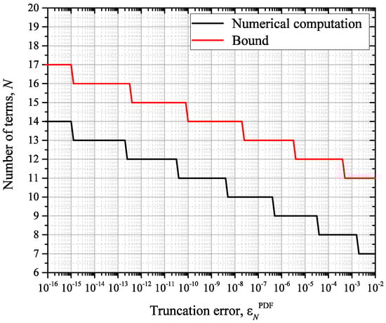
Figure 1. Required number of terms computed numerically and using the bound given by (17).

On the other hand, this figure presents the required number of terms in the summation when the termination criterion is an absolute value of the first term left after terminating the summation to be less than ${\epsilon }_N^{PDF}$. In other words, if we denote the $(N+1)$th term of the series by $b_{N+1}={(-1)}^{N+1}{\mathrm{I}}_m\left(r{V}_1/{\sigma }_F^2\right){\mathrm{I}}_m\left(r{V}_2/{\sigma }_F^2\right){\mathrm{I}}_m\left(V_1{V}_2/{\sigma }_F^2\right)$, we perform the summation until the condition $|b_{N+1}|\le {\epsilon }_N^{\mathrm{PDF}}$ is satisfied. It is clear that the required number of terms estimated on the basis of (17) is larger than the number of terms determined under the condition that the absolute value of the first term left after terminating the summation is less than ${\epsilon }_N^{PDF}$. That means we have derived a bound on the truncation error which gives us the required number of terms in the summation to be sure that a given accuracy will be satisfied.

Based on the results from Figure 1, it can be noted that the same number of terms in the summation is needed to reach the bound for the truncation error in the range of several orders of magnitude. For example, 16 terms are necessary to ensure the bound on the truncation error from $2\times {10}^{-15}$ to $3\times {10}^{-13}$ This is the consequence of the number of terms being an integer value, which leads to the step-like behavior in Figure 1.

3.2. Convergence Analysis of Series in CDF

As in the case of the PDF considered in the previous subsection, in this subsection, we derive the upper bound for the absolute truncation error when evaluating the CDF given by (11) and we derive the formula for the required number of terms to achieve a given accuracy in the summation in (11).

3.2.1. Truncation Error of Series in CDF

Here, we can also apply the alternating series estimation theorem bounding the absolute truncation error on the upper side to the absolute value of the first term left out after stopping the summation [15]. In estimating the truncation error in (11), we focus on series

$$S_2=\sum _{m=1}^{+\infty }{\displaystyle \frac{{(-1)}^m}{m!}}{\left({\displaystyle \frac{V_1^2}{2{\sigma }_F^2}}\right)}^m{}_2{F}_1\left(-m,-m;1;{\displaystyle \frac{V_2^2}{V_1^2}}\right){}_1{F}_1\left(1-m;2;{\displaystyle \frac{r^2}{2{\sigma }_F^2}}\right)$$

(29)

The truncation error of series $S_2$ is

$${\epsilon }_N^{CDF}=\sum _{m=N+1}^{+\infty }{\displaystyle \frac{{(-1)}^m}{m!}}{\left({\displaystyle \frac{V_1^2}{2{\sigma }_F^2}}\right)}^m{}_2{F}_1\left(-m,-m;1;{\displaystyle \frac{V_2^2}{V_1^2}}\right){}_1{F}_1\left(1-m;2;{\displaystyle \frac{r^2}{2{\sigma }_F^2}}\right)$$

(30)

Proposition 3.

The upper bound for the truncation error ${\epsilon }_N^{CDF}$ defined by (30) is given by

$$\left|{\epsilon }_N^{CDF}\right|\le R_N^{CDF}=\left(\genfrac{}{}{0pt}{}{N-1/2}{N+1}\right){\displaystyle \frac{{\left[2a(1+b)\right]}^{N+1}}{(N+1)!}}{\displaystyle \frac{{({((N+1)!)}^{1/N}+c)}^N}{(N+1)!}}.$$

(31)

where the parameters are defined as $a=V_1^2/\left(2{\sigma }_F^2\right)$, $b=V_2^2/V_1^2$ and $c=r^2/\left(2{\sigma }_F^2\right)$.

Proof of Proposition 3.

In order to estimate the upper bound for the truncation error and the required number of terms in the series to achieve a given absolute accuracy, we derive the bound for the hypergeometric functions appearing in (29).

• Derivation of the upper bound for function ${}_2{F}_1\left(-m,-m;1;z\right)$.

Based on ([24], (07.23.03.0195.01)), it holds that

$${}_2{F}_1\left(-m,-m;1;z\right)={(1-z)}^m{P}_m\left({\displaystyle \frac{1+z}{1-z}}\right)$$

(32)

where $P_m\left(x\right)$ denotes the Legendre polynomial defined in ([16], (8.910)). We start the derivation of the bound for the hypergeometric function in (29) by proving the equality

$$|P_m\left(x\right)|<a_m{\left|x\right|}^m,$$

(33)

where $a_m$ denotes the coefficient with $x_m$ in the Legendre polynomial of order m. The coefficient $a_m$ can be expressed as ([25], p. 40)

$$a_m={\displaystyle \frac{\left(2m\right)!}{2^m{(m!)}^2}}=2^m\left(\genfrac{}{}{0pt}{}{m-1/2}{m}\right)$$

(34)

Since the zeros of Legendre polynomials are real and symmetrical, we write

$$P_m\left(x\right)=a_m{x}^{(1+{(-1)}^{m+1})/2}\prod _{i=0}^{\lfloor m/2\rfloor }(x^2-{\alpha }_i^2),$$

(35)

where ${\alpha }_i$ are zeros of the Legendre polynomial of order m. The polynomials of odd order have an additional zero which is located at $x=0$. All zeros are located inside the interval $(-1,1)$, implying $0\le {\alpha }_i^2<1$ and therefore $|x^2-{\alpha }_i^2|<x^2$ when $x>1$, so we can directly write

$$|P_m\left(x\right)|<a_m{\left|x\right|}^m,\left|x\right|>1,m>1$$

(36)

Since $-1\le P_m\left(x\right)\le 1$, for $-1\le x\le 1$, we can extend the inequality to arbitrary real x in the following way

$$|P_m\left(x\right)|<1+a_m{\left|x\right|}^m,m>1$$

(37)

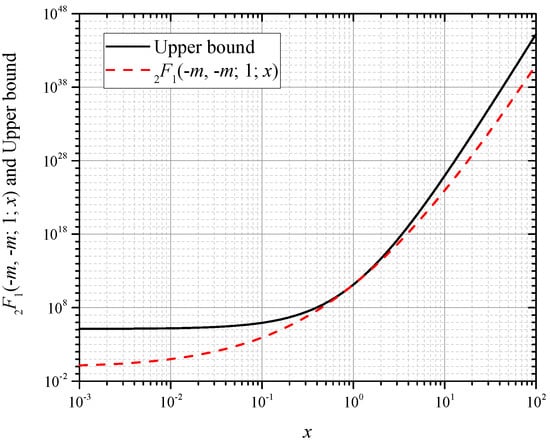
Since $(1+x)/(1-x)\ge 1$ when $0\le x<1$, we use the first version (36) of the inequality, yielding

$${}_2{F}_1\left(-m,-m;1;x\right)\le a_m{(1+x)}^m,x\ge 0,$$

(38)

where equality is achieved at x = 1. This derived inequality (38) is illustrated in Figure 2.

Figure 2. Simple upper bound for ${}_2{F}_1(-m,-m;1;x)$, for $m=20$.

• Derivation of the upper bound for function ${}_1{F}_1\left(1-m;2;z\right)$.

A confluent hypergeometric function can be represented as ([24], (07.03.26.0002.01), (07.20.27.0001.01))

$${}_1{F}_1\left(1-m;2;z\right)={\displaystyle \frac{1}{m}}{L}_{m-1}^1\left(z\right).$$

(39)

where $L_m^{\alpha }\left(z\right)$ represents the Laguerre function [16]. Love noted in [26] that there were only a few results published about Laguerre polynomials’ inequalities. Our result in this context is stated as:

$${\displaystyle \frac{1}{m}}\left|L_{m-1}^1\left(z\right)\right|\le {\displaystyle \frac{1}{m!}}{(\alpha (m-1)+z)}^{m-1}={\displaystyle \frac{b_{m-1}^{\left(1\right)}\left(z\right)}{m}},\alpha (m-1)={(m!)}^{1/(m-1)}.$$

(40)

Using ([27], (5.17)), we get

$$L_m^1\left(0\right)=m+1.$$

(41)

By substituting $z=0$ into the previous inequality, we get

$$\left|L_{m-1}^1\left(0\right)\right|=m\le {\displaystyle \frac{1}{(m-1)!}}\alpha {(m-1)}^{m-1},$$

(42)

which yields an appropriate value for $\alpha \left(m\right)$, as

$$\alpha \left(m\right)={((m+1)!)}^{1/m}.$$

(43)

All the zeros of Laguerre polynomials are positive, so we can prove

$$\left|L_m^1\left(z\right)\right|<{\displaystyle \frac{1}{m!}}{z}^m,$$

(44)

when z is larger than the largest zero of $L_m^1\left(z\right)$. Therefore,

$${\displaystyle \frac{1}{m}}\left|L_{m-1}^1\left(z\right)\right|\le {\displaystyle \frac{1}{m!}}{(\alpha (m-1)+z)}^{m-1},z>z_1,$$

(45)

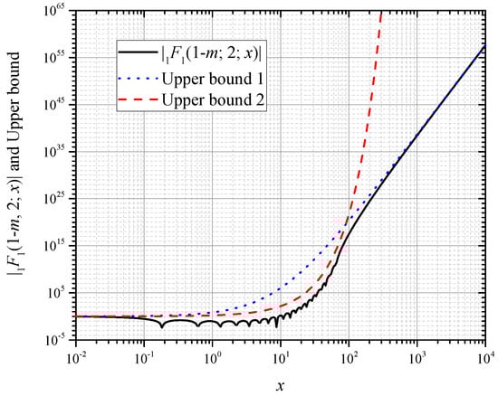
where $z_1$ is the largest zero of $L_{m-1}^1\left(z\right)$. Another bound can be proven for Laguerre polynomials, ([28], 10.18(14)), ([29], (18.14.8))

$$\left|L_m^1\left(x\right)\right|\le (m+1)exp{\displaystyle \frac{x}{2}}=b_m^{\left(2\right)}\left(x\right),z>0.$$

(46)

An illustration of the two bounds is shown in Figure 3. It can be seen that the bound $b_m^{\left(1\right)}\left(z\right)$ is valid, but not as sharp as $b_m^{\left(2\right)}\left(z\right)$ for smaller values of z that are below the largest zero. On the other hand, for large z, the bounds’ sharpness is reversed.

Figure 3. Two upper bounds for $|{}_1{F}_1(1-m;2;x)|$, for $m=20$.

On the basis of the previously derived formulas and the alternative series truncation error theorem, Proposition 3 is proven. □

Corollary 2.

On the basis of (31), it is evident that $\underset{x\to +\infty }{lim}{R}_N^{CDF}=0$, which means the series $S_2$ given by (29) is convergent.

Regarding Figure 3, the crossing point $x_0$ between the two bounds can be used in the following statement:

$$\mathrm{bound}=\left\{\begin{array}{cc}\mathrm{bound}2,\hfill & 0\le x<x_0\hfill \\ \mathrm{bound}1,\hfill & x_0\le x<+\infty \hfill \end{array}\right.$$

(47)

To date, we have not seen in the literature this exact combination of bounds addressing the $[0,\infty )$ range. Additionally, the crossing point can be expressed in closed*form as

$${\displaystyle \frac{x_0}{2m}}=-{\beta }_m-W_{-1}\left(-{\beta }_m{\mathrm{e}}^{-{\beta }_m}\right),$$

(48)

where ${\beta }_m={\displaystyle \frac{{((1+m)!)}^{1/m}}{2m}}$.

3.2.2. Required Number of Terms for Evaluating CDF

In this subsection, we derive two formulas giving an explicit relation between the required number of terms in the summation, and the value of the absolute truncation error. One equation is marked as “Upper bound 1”, and the other is marked as “Upper bound 2”.

Proposition 4.

The required number ($N_1$) of terms in the summation in (29) under the condition of achieving absolute truncation error ${\epsilon }_N^{CDF}$ can be determined by $N=\lceil m\rceil$

$$m\ge \left\{\begin{array}{cc}{\displaystyle \frac{2\mathrm{e}c+log{\displaystyle \frac{1}{2{\pi }^2{\left({\epsilon }_N^{CDF}\right)}^2}}}{2W\left({\displaystyle \frac{1}{4a(1+b)\mathrm{e}}}(2\mathrm{e}c+log{\displaystyle \frac{1}{2{\pi }^2{\left({\epsilon }_N^{CDF}\right)}^2}})\right)}}\hfill & {\epsilon }_N^{CDF}<{\epsilon }_1={\displaystyle \frac{1}{\pi }}{\left({\displaystyle \frac{1}{2}}{\mathrm{e}}^{4a(1+b)+2\mathrm{e}c}\right)}^{1/2}\hfill \\ 2a(1+b),\hfill & {\epsilon }_N^{CDF}={\epsilon }_1\hfill \\ 0,\hfill & \mathit{otherwise}\hfill \end{array}\right.,$$

(49)

where $a={\displaystyle \frac{V_1^2}{2{\sigma }_F^2}}$, $b={\displaystyle \frac{V_2^2}{V_1^2}}$ and $c={\displaystyle \frac{r^2}{2{\sigma }_F^2}}$.

Proof of Proposition 4.

By regarding the generalized binomial coefficient as

$$\left(\genfrac{}{}{0pt}{}{m}{n}\right)={\displaystyle \frac{\mathsf{\Gamma }(m+1)}{\mathsf{\Gamma }(n+1)\mathsf{\Gamma }(m-n+1)}}m,n,m-n\notin {\mathbb{Z}}_0^{-},$$

(50)

and expanding $\left(\genfrac{}{}{0pt}{}{m-1/2}{m}\right)$ into a series around $m\to +\infty$, we get

$$\left(\genfrac{}{}{0pt}{}{m-1/2}{m}\right)={\displaystyle \frac{1}{\sqrt{m\pi }}}+O\left(m^{-3/2}\right).$$

(51)

It can be proved that the following holds

$${\displaystyle \frac{1}{\sqrt{m\pi }}}\ge \left(\genfrac{}{}{0pt}{}{m-1/2}{m}\right)$$

(52)

Unfortunately, after the previous simplification, (31) is still too complex for symbolic manipulation. In order to obtain results with a reasonable complexity, we use the limit

$$\underset{m\to +\infty }{lim}{\displaystyle \frac{{({(m!)}^{1/(m-1)}+c)}^{m-1}}{m!}}=exp\left(\mathrm{e}c\right).$$

(53)

Our upper bound is now

$$R_{m-1}^{CDF}\approx {\displaystyle \frac{{\left[2a(1+b)\right]}^m}{m!}}{\displaystyle \frac{exp\left(\mathrm{e}c\right)}{\sqrt{m\pi }}}<{\displaystyle \frac{{\left[2a(1+b)\right]}^m}{m!}}{\displaystyle \frac{exp\left(\mathrm{e}c\right)}{\sqrt{\pi }}},m>1.$$

(54)

This leads to an equation for m given by

$${\displaystyle \frac{exp\left(\mathrm{e}c\right)}{\pi \sqrt{2}}}{\left({\displaystyle \frac{2a(1+b)\mathrm{e}}{m}}\right)}^m\le \epsilon .$$

(55)

The variable m can be expressed similarly as it was in the case of the PDF. The solution is given by (49). We note that the limiting value is

$$\underset{\epsilon \to {\epsilon }_1^{-}}{lim}{\displaystyle \frac{2\mathrm{e}c+log{\displaystyle \frac{1}{2{\pi }^2{\epsilon }^2}}}{2W\left({\displaystyle \frac{1}{4a(1+b)\mathrm{e}}}\left(2\mathrm{e}c+log{\displaystyle \frac{1}{2{\pi }^2{\epsilon }^2}}\right)\right)}}=2a(1+b),$$

(56)

and for $\epsilon >{\epsilon }_1$, the required m is $m\ge 0$. □

Proposition 5.

The required number ($N_2$) of terms in the summation in (29) under the condition of achieving the truncation error can be determined by $N=\lceil m\rceil$

$$m\ge \left\{\begin{array}{cc}{\displaystyle \frac{c+log{\displaystyle \frac{1}{2{\pi }^2{\left({\epsilon }_N^{CDF}\right)}^2}}}{2W\left({\displaystyle \frac{1}{4a(1+b)\mathrm{e}}}(c+log{\displaystyle \frac{1}{2{\pi }^2{\left({\epsilon }_N^{CDF}\right)}^2}})\right)}}\hfill & {\epsilon }_N^{CDF}<{\epsilon }_2={\displaystyle \frac{1}{\pi }}{\left({\displaystyle \frac{1}{2}}{\mathrm{e}}^{4a(1+b)+c}\right)}^{1/2}\hfill \\ 2a(1+b),\hfill & {\epsilon }_N^{CDF}>{\epsilon }_2\hfill \\ 0,\hfill & \mathit{otherwise}\hfill \end{array}\right.,$$

(57)

where $a={\displaystyle \frac{V_1^2}{2{\sigma }_F^2}}$, $b={\displaystyle \frac{V_2^2}{V_1^2}}$ and $c={\displaystyle \frac{r^2}{2{\sigma }_F^2}}$. This solution is denoted by “Upper bound 2”.

Proof of Proposition 5.

By direct use of (46), it follows that

$${\displaystyle \frac{a^m}{m!}}{}_2{F}_1\left(-m,-m;1;b\right)\left|{}_1{F}_1\left(1-m;2;c\right)\right|<\left(\genfrac{}{}{0pt}{}{m-1/2}{m}\right){\displaystyle \frac{{\left[2a(1+b)\right]}^m}{m!}}exp(c/2),$$

(58)

From inequality (58), (57) follows. □

By comparing (49) with (57), we can notice that the latter is obtained by substituting c with $c/\left(2\mathrm{e}\right)$ in the former.

Figure 4 presents the required number of terms (both $N_1$ and $N_2$) needed to achieve a given absolute truncation error. This figure also presents the required number of terms that is determined from the criterion that the summation be terminated when the absolute value of the next term is less than ${\epsilon }_N^{CDF}$.

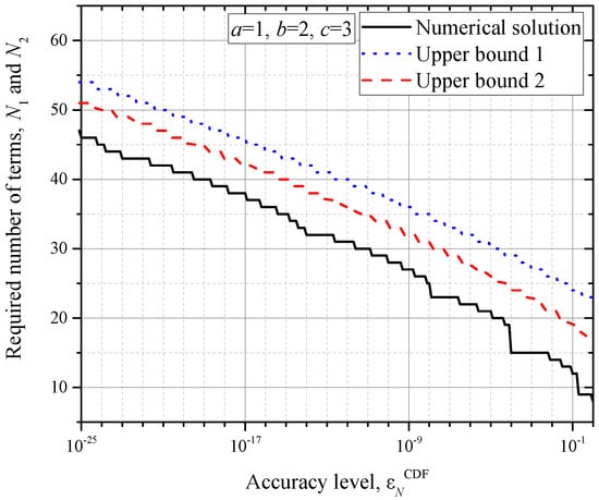
Figure 4. Illustration of the required number of terms in the summation in the CDF to achieve a specified absolute truncation error.

Figure 4 illustrates the required number of terms in the sum in (29). Firstly, we estimated the number of terms numerically in a way that we terminated the summation when the absolute value of the first term left after the summation was less than the accuracy level denoted by ${\epsilon }_N^{CDF}$. Secondly, we determined the number of terms was the summation based on (49), and that value was denoted as “Upper bound 1”. Thirdly, we estimated the number of terms based on (57). That bound was denoted as “Upper bound 2”. It is clear that the values that were estimated numerically are closer to the values estimated based on (57) compared with those estimated based on (49).

4. Numerical Results and Discussion

In the previous section, we derived new closed-form expressions ((13) and (30)) for the upper bounds of the truncation errors when evaluating the PDF and CDF of the signal envelope. These expressions were derived in terms of elementary mathematical functions. In addition, we derived closed-form Formulas (17), (49) and (57) giving a straightforward relation between the number of terms in the summation on one hand, and the value of the truncation error and channel parameters on the other hand. In this section, we give some illustrations of applications of these formulas.

Figure 5 and Figure 6 present the numerical values of the upper bounds for the truncation error of the PDF under different channel conditions. Figure 5a presents the upper bound for the truncation error vs. the required number of terms in the summation to achieve this upper bound. We present several curves corresponding to different values of parameter K. The larger the value of parameter K, the larger the number of terms necessary to achieve the given bound for the truncation error. For example, to achieve the bound for a truncation error of ${10}^{-12}$, the required number of terms in the summation increases from $N=8$ to $N=21$ when parameter K increases from $K=4$ dB to $K=12$ dB. In other words, a larger number of terms is required in channels with stronger specular components compared with the diffuse component. Figure 5b presents the dependence of the required number of terms in the summation vs. the truncation error. This dependence is given by (17). For values of the truncation error of ${10}^{-12}$, the required numbers of terms according to (17) are 10 and 23. We can conclude that relation (17) gives numbers of terms larger than those numbers that can be noticed from the dependence in Figure 5a, which were obtained based on (14).

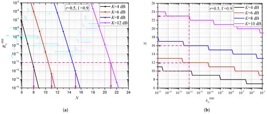
Figure 5. Effect of parameter K on accuracy of evaluating PDF: (a) upper bound for truncation error vs. number of terms in summation; (b) required number of terms vs. truncation error.

Figure 6. Effect of parameter $\mathsf{\Gamma }$ on accuracy of evaluating PDF: (a) upper bound for truncation error vs. number of terms in summation; (b) required number of terms vs. truncation error.

The influence of parameter $\mathsf{\Gamma }$ on the number of required terms for achieving a given upper bound for the truncation error is illustrated in Figure 6. The larger the value of parameter $\mathsf{\Gamma }$, the larger the number of terms in the summation required to achieve a given upper bound for the truncation error. If we fix the bound for the truncation error to ${10}^{-12}$, from Figure 6a, we can read that it is necessary to sum $N=10$ and $N=15$ terms if $\mathsf{\Gamma }=0.2$ and $\mathsf{\Gamma }=1$, respectively. When applying (17), i.e., from the results presented in Figure 6b, we conclude that for a truncation error of ${10}^{-12}$, relation (17) gives the estimation that it is necessary to have 11 and 16 terms in the summation. As it was highlighted during the derivation, (17) gives overestimated values compared with those values that can be read from the dependence defined by (14).

The effect of channel conditions on the required terms when evaluating a CDF value is illustrated in Figure 7. The high values of parameter K mean that a larger number of terms is required, as in the case of evaluating a PDF value. As in the case of evaluating PDF, the same conclusions are derived from the results presented in the figure. Relation (57), linking the required number of terms in the summation vs. the truncation error, gives overestimated values of the number of terms compared with those values that can be read from the dependence of the bounds for the truncation error vs. the number of terms, which are defined by (31). When comparing the results from Figure 5 and Figure 7, we can conclude that a larger number of terms is required when evaluating the CDF in comparison with the number of terms when evaluating the PDF, for the same conditions.

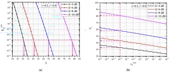
Figure 7. Effect of parameter K on accuracy of evaluating CDF: (a) upper bound for truncation error vs. number of terms in summation; (b) required number of terms vs. truncation error.

Figure 8 presents PDF curves that were evaluated based on (10), when the number of terms in the summation was estimated under the condition that the upper bound of the truncation error be less than ${10}^{-12}$. The PDF curves obtained by simulations are also presented in Figure 8. These simulation results were estimated based on samples generated according to (3). The samples were generated in the software package Mathematica 13. Uniform and Gaussian random numbers were generated by using built-in subroutines in Mathematica 13. When showing the histograms of the Monte Carlo data, we used linearly distributed bins with a total bin count of 200, and a total number of simulation points of ${10}^6$. The standard deviation of the histogram relative to numerically computed values of the distribution was $\sigma =0.008$ for the 10 dB case and $\sigma =0.0062$ for 4 dB. It is visible that the analytical and simulation results are in agreement, which is a confirmation that the suggested estimation of the required number of terms in the summation presented in this paper is correct.

Figure 8. Analytical and Monte Carlo simulation results.

5. Conclusions

By applying the alternating series estimation theorem, we derived novel formulas for the upper bounds for the absolute truncation error when evaluating the PDF and CDF of a composite signal envelope transmitting over $\mathrm{m}$$\mathrm{m}$-Wave channels. In addition, we derived novel analytical expressions giving the required number of terms in the infinity sums in the PDF and CDF under the condition of achieving a given absolute accuracy. In deriving these main formulas, we first derived two formulas for the upper bounds for the special functions ${}_2{F}_1\left(-m,-m;1;·\right)$ and ${}_1{F}_1\left(1-m;2;·\right)$, where some properties of orthogonal polynomials were used. All the formulas were derived in terms of elementary mathematical functions. Based on the results presented here, both series (in the PDF and CDF) converged fast and for all practical channel parameters, it was enough to evaluate up to 100 terms in order to achieve an absolute accuracy of ${10}^{-12}$. A larger number of terms was required for evaluating the CDF in comparison with the number of terms required for evaluating the PDF, for the same channel conditions. To verify the analytical results, when evaluating PDF curves, we used in the summation the required number of terms predicted by the formulas derived here. These analytical curves were verified by independent Monte Carlo simulations. The results will have an important role in contemporary wireless communications theory for the design and analysis of beyond-5G networks.

References

- Simon, M.K.; Alouini, M.S. Digital Communication over Fading Channels, 2nd ed.; John Wiley & Sons, Inc.: Hoboken, NJ, USA, 2004. [Google Scholar] [CrossRef]
- Shankar, P.M. Fading and Shadowing in Wireless Systems, 2nd ed.; Springer: Cham, Switzerland, 2017. [Google Scholar] [CrossRef]
- Mavridis, T.; Petrillo, L.; Sarrazin, J.; Benlarbi-Delai, A.; De Doncker, P. Near-body shadowing analysis at 60 GHz. IEEE Trans. Antennas Propag. 2015, 63, 4505–4511. [Google Scholar] [CrossRef]
- Kim, D.; Lee, H.; Kang, J. Comments on “Near-body shadowing analysis at 60 GHz”. IEEE Trans. Antennas Propag. 2017, 65, 3314. [Google Scholar] [CrossRef]
- Zöchmann, E.; Caban, S.; Mecklenbräuker, C.F.; Pratschner, S.; Lerch, M.; Schwarz, S.; Rupp, M. Better than Rician: Modelling millimetre wave channels as two-wave with diffuse power. EURASIP J. Wirel. Commun. Netw. 2019, 2019, 1–17. [Google Scholar] [CrossRef]
- Sánchez, J.D.V.; Urquiza-Aguiar, L.; Paredes Paredes, M.C. Fading channel models for mm-wave communications. Electronics 2021, 10, 798. [Google Scholar] [CrossRef]
- Durgin, G.D.; Rappaport, T.S.; De Wolf, D.A. New analytical models and probability density functions for fading in wireless communications. IEEE Trans. Commun. 2002, 50, 1005–1015. [Google Scholar] [CrossRef]
- Kim, D.; Lee, H.; Kang, J. Comprehensive analysis of the impact of TWDP fading on the achievable error rate performance of BPSK signaling. IEICE Trans. Commun. 2018, 101, 500–507. [Google Scholar] [CrossRef]
- Rao, M.; Lopez-Martinez, F.J.; Alouini, M.S.; Goldsmith, A. MGF approach to the analysis of generalized two-ray fading models. IEEE Trans. Wirel. Commun. 2015, 14, 2548–2561. [Google Scholar] [CrossRef]
- Lopez-Fernandez, J.; Moreno-Pozas, L.; Lopez-Martinez, F.J.; Martos-Naya, E. Joint parameter estimation for the two-wave with diffuse power fading model. Sensors 2016, 16, 1014. [Google Scholar] [CrossRef] [PubMed]
- Maric, A.; Kaljic, E.; Njemcevic, P. An alternative statistical characterization of TWDP fading model. Sensors 2021, 21, 7513. [Google Scholar] [CrossRef] [PubMed]
- Njemcevic, P.; Kaljic, E.; Maric, A. Moment-Based Parameter Estimation for the Γ-Parameterized TWDP Model. Sensors 2022, 22, 774. [Google Scholar] [CrossRef] [PubMed]
- Kostic, I. Envelope probability density function of the sum of signal, noise and interference. Electron. Lett. 1978, 14, 490–491. [Google Scholar] [CrossRef]
- Kostic, I. Cumulative distribution function of envelope of sum of signal, noise and interference. In Proceedings of the Telecommunication Forum (TELFOR), Belgrade, Yugoslavia, 26–28 November 1996; pp. 301–303. [Google Scholar]
- Milovanovic, G.V. Numerical Analysis, Part I; University of Nis: Nis, Yugoslavia, 1979. (In Serbian) [Google Scholar]
- Gradshteyn, I.S.; Ryzhik, I.M. Table of Integrals, Series, and Products, 6th ed.; Academic Press: New York, NY, USA, 2000. [Google Scholar]
- Choi, J.; Milovanović, G.V.; Rathie, A.K. Generalized summation formulas for the Kampé de Fériet function. Axioms 2021, 10, 318. [Google Scholar] [CrossRef]
- Luke, Y.L. Inequalities for generalized hypergeometric functions. J. Approx. Theory 1972, 5, 41–65. [Google Scholar] [CrossRef]
- Joshi, C.; Bissu, S. Some inequalities of Bessel and modified Bessel functions. J. Aust. Math. Soc. 1991, 50, 333–342. [Google Scholar] [CrossRef][Green Version]
- Corless, R.M.; Gonnet, G.H.; Hare, D.E.; Jeffrey, D.J.; Knuth, D.E. On the LambertW function. Adv. Comput. Math. 1996, 5, 329–359. [Google Scholar] [CrossRef]
- Lóczi, L. Guaranteed-and high-precision evaluation of the Lambert W function. Appl. Math. Comput. 2022, 433, 127406. [Google Scholar] [CrossRef]
- Iacono, R.; Boyd, J.P. New approximations to the principal real-valued branch of the Lambert W-function. Adv. Comput. Math. 2017, 43, 1403–1436. [Google Scholar] [CrossRef]
- Howard, R.M. Analytical Approximations for the Principal Branch of the Lambert W Function. Eur. J. Math. Anal. 2022, 2, 14. [Google Scholar] [CrossRef]
- Wolfram Research, Inc. The Mathematical Functions Site. 1998–2022. Available online: http://functions.wolfram.com (accessed on 15 August 2022).
- Milovanovic, G.; Mitrinovic, D.; Rassias, T. Topics in Polynomials: Extremal Problems, Inequalities, Zeros; World Scientific: Singapore, 1994. [Google Scholar] [CrossRef]
- Love, E. Inequalities for Laguerre functions. J. Inequalities Appl. 1997, 1997, 936095. [Google Scholar] [CrossRef]
- Szegö, G. Orthogonal Polynomials, 4th ed.; American Mathematical Society, Colloquium Publications: Providence, RI, USA, 1975; Volume 23. [Google Scholar] [CrossRef]
- Erldelyi, A.; Magnus, W.; Oberhettinger, F.; Tricomi, F. Higher Transcendental Functions; McGraw-Hill: New York, NY, USA, 1955; Volume 2. [Google Scholar]
- NIST Digital Library of Mathematical Functions; Release 1.1.6 of 2022-06-30; Olver, F.W.J., Daalhuis, A.B.O., Lozier, D.W., Schneider, B.I., Boisvert, R.F., Clark, C.W., Miller, B.R., Saunders, B.V., Cohl, H.S., McClain, M.A., Eds.; Available online: http://dlmf.nist.gov/ (accessed on 30 June 2022.).
Publisher’s Note: MDPI stays neutral with regard to jurisdictional claims in published maps and institutional affiliations. |
© 2022 by the authors. Licensee MDPI, Basel, Switzerland. This article is an open access article distributed under the terms and conditions of the Creative Commons Attribution (CC BY) license (https://creativecommons.org/licenses/by/4.0/).