A Study of Stopping Rules in the Steepest Ascent Methodology for the Optimization of a Simulated Process

Abstract

Competitiveness motivates organizations to implement statistical approaches for improvement purposes. The literature offers a variety of quantitative methods intended to analyze and improve processes such as the design of experiments, steepest paths and stopping rules that search optimum responses. The objective of this paper is to run a first-order experiment to develop a steepest ascent path to subsequently apply three stopping rules (Myers and Khuri stopping rule, recursive parabolic rule and recursive parabolic rule enhanced) to identify the optimum experimentation stop from two different simulated cases. The method includes the consideration of the case study, the fitting of a linear model, the development of the steepest path and the application of stopping rules. Results suggest that procedures’ performances are similar when the response obeys a parametric function and differ when the response exhibits stochastic behavior. The discussion section shows a structured analysis to visualize these results and the output of each of the stopping rules in the two analyzed cases.

1. Introduction

Today’s industry demands more optimization in its processes. Weichert et al. [1] assure that advances in the manufacturing industry and the resulting available data have brought important progress and large interest in optimization-related methods to improve production processes. In several different disciplines, engineers have to take many technological and managerial decisions at different stages for optimization purposes. The literature shows different examples of this, such as the case of [2,3,4], with research that successfully involves optimization for different purposes. The ultimate goal is either to minimize the effort required or to maximize the desired benefit. For instance, Balafkandeh et al. [5] and Juangphanich et al. [6] focus their efforts on optimizing operations to minimize outputs, while, Oleksy-Sobczak and Klewicka [7] and Delavar and Naderifar [8] pursue optimization of inputs to maximize results.

However, companies are not only concerned with creating more products with less resources; they also have the intention of performing right operations the first time. Several organizations around the world use statistical approaches as the core of process problem solving. According to Bryant [9], problem solving constitutes the ambition to transcend the limits of ordinary capability, sometimes against rational ideas and the limitation of human capabilities, because people still have the need to reduce potential complexity and manage cognitive load. Inside an industrial environment, problem solving is widely related to productivity and it is an everyday issue to solve. In this scenario, each company is responsible for its own development. As noted by Apsemidis et al. [10], the complexity of the industrial environment may be large enough to avoid classical process monitoring techniques and substitute new statistical learning methodologies. This is why mathematical and statistical approaches are being designed for organizations to obtain higher performance in their processes.

There are several quantitative methods such as Design Of Experiments (DOE), intended to analyze and improve processes. As explained by Montgomery [11], experiments are useful to understand the performance of a process or any system that combines operations, machines, methods, people and other resources to transform some inputs (commonly a material) into an output with one or more observable response variables. Likewise, experimental designs have found several methods of learning through a series of activities, with the aim of making conjectures about a process to drive innovation in the product realization process, resulting in improvement of process yield, reduction of variability, closer conformance to nominal, reduction of development time and, finally, reducing costs by the optimization of processes.

For instance, Sheoran and Kumar [12] studied a set of processing parameters that needed to be carefully selected for a specific output requirement. It was noted that some of these parameters were more significant for the response variable than the rest; this significance needed to be identified and optimized. Therefore, researchers explored different experimental or statistical approaches such as DOE for optimization and property improvement purposes.

The task of optimizing systems is always complex because of the quantity of factors involved. Beyond DOE, there is a method called Response Surface Methodology (RSM) used for this purpose. As stated by Myers et al. [13], a RSM is a collection of statistical techniques useful for developing, improving and optimizing a process. In the case of industrial processes, it is very useful to apply this method particularly in situations where different input variables influence the performance or quality characteristics of the product (the response variable). This method is useful in the solution of several problems such as mapping a response surface over a particular region of interest, selection of operating conditions to achieve specifications, customer requirements and, of course, optimization of a response.

For example, Karimifard and Moghaddam [14] presents RSM as a powerful tool for designing experiments and analyzing processes related to different environmental wastewater treatment operations with successfully optimized outputs.

Beyond these strategic tools, an auxiliary method to analyze the behavior of a response is called the Steepest Ascent or Descent Method (SADM). It is useful to obtain a region where optimization is feasible. Myers et al. [13] remarks that this method searches for such regions through experimental design, model-building procedure and sequential experimentation. The type of designs that are most frequently used are the two-level factorial and fractional factorial designs. It is fundamental to remember that the strategy involves sequential movement in the factors from one region to another, resulting in more than one experiment. As mentioned by De Oliveira et al. [15], optimization of processes commonly involves statistical techniques such as the RSM as one of the most effective ways to pursue optimization by modeling techniques.

A great exemplification of this is application of SADM by Chavan and Talange [16], who applied a full factorial statistical design to obtain a model to find which input factors affect the response variables significantly in a process of fuel cells. The steepest ascent method was applied to find the maximum power delivered by these fuel cells within the defined ranges of input factors.

Since the SADM entails consecutive individual experimentation, it becomes necessary to have a procedure that gives mathematical support to recognize when the response has been improved and no more experimentation needs to be carried out. They are called Stopping Rules (SRs).

Myers and Khuri [17] presented a procedure that consists in performing a sequence of sets of trials with the information provided by the first-order fitting. This Myers and Khuri Stopping Rule (MKSR) is used to determine a path to observe an increasing or decreasing response. This procedure considers the random error variation in the response and avoids the need to take many observations when the true mean response is decreasing. Furthermore, it prevents premature stopping decisions when the true mean response is decreasing. The stopping procedure is applied once a steepest path is developed and has been used in experimental strategy in optimum seeking methodology. There have been different informal procedures to stop, such as one that orders a stop at the first drop. Another informal tendency has been stopping after three consecutive drops. Nevertheless, due to the presence of random error variation in the observed response, the dropping of the response may not be true all along the function. Therefore, the need to design formal rules such as the MKSR has been important. The most important characteristic of the MKSR is that it assumes that $y\left(t\right)$ is normally distributed with mean $\eta \left(t\right)$ and variance ${\sigma }^2$ from a sequence of independent normal variables.

Similarly, Miró-Quesada and Del Castillo [18] reported that a first-order experimental design is commonly followed by a steepest ascent search where there is a need for a stopping rule to determine the optimal point in the search direction. This procedure, known as Del Castillo’s Recursive Parabolic Rule (RPR), has been studied for quadratic responses. It is assumed that it is of interest to maximize the response, so the steepest ascent case is considered. In real experimentation, stopping a search before the maximum response over a path means that the optimum value will not be selected and the procedure will not be able to be efficient because of the wasting of resources in experimentation. One of the most important considerations when applying the RPR is that this procedure tries to fit a quadratic behavior to the observed data. It also recursively updates the estimate of the second-order coefficient and tests if the first derivative is negative. However, the necessity of developing a more robust procedure to also consider non-quadratic behavior is starting to be an important issue to solve.

Finally, Del Castillo [19] explains a procedure to also consider non-quadratic behavior, called the Recursive Parabolic Rule Enhanced (RPRE). It has the advantage of being more robust because it becomes more sensitive when the standard deviation of the error is small. It mainly consists of three modifications to the traditional recursive rule. The intercept and the first order term, in addition to the second term, are recursively fitted. Furthermore, only a local parabolic model along the search direction is fitted, defined by a new concept called window. Finally, a coding scheme on the numbers of steps is used to reduce variance.

In this paper, a comprehensive study is carried out. It considers two simulated processes that offer response variables after a set of inputs (different levels and factors) configured according to a factorial design. The application and comparison of the mentioned three SRs will be illustrated, with the objective of recognizing the best performance. This analysis is important and relevant considering that current literature lacks recent studies of this nature, where three of the most important formal stopping rules are applied over a path of improvement that considers the coefficients of a linear model. This study is characterized by its lack of comparability with previous studies, because the response variables obtained by the simulators applied were specially obtained for this particular experiment. This means that comparison with previous studies is not feasible, since it can only be applied to the special conditions where responses were exclusively obtained for this case.

At this point, the originality of the contribution of this paper not only relies on the verification and comparison of performance of SRs, but also on the interaction of SRs with the behavior of the outputs. SR performance is similar when the response obeys a parametric function and differs when the output follows a stochastic behavior. It is important that further analysis over stochastic behaviors continue to pursue an even better procedure to stop over the path of improvement.

After this first section of introduction, Section 2 is intended to show the method used for the paper and explain the application of rules. Section 3 presents the results obtained with both of the cases after the application of the three SRs. Finally, discussion and conclusion are presented in Section 4 and Section 5, respectively.

2. Method

This procedure is intended to follow the main objective, which consists in running a first-order designed experiment and subsequently performing a steepest ascent/descent. The core of this analysis is to run the SRs previously addressed to discover the best performance between the MKSR, the RPR and the RPRE under the conditions of the specific experimentation schemes and cases considered.

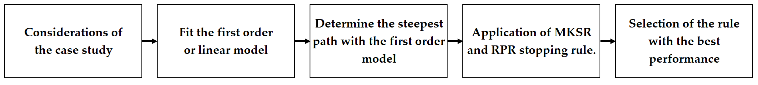
The method is explained in Figure 1 as a flow chart to easily visualize the progress.

The first stage of the method consists in the considerations of the three cases that will be presented. Second, the first-order model is fitted; a linear regression equation is used. Then, the steepest path with the first-order model is determined so that the application of the MKSR, RPR and RPRE is possible. Finally, the selection of the rule with the best performance is denoted for each of the analyzed cases.

a. Considerations of the case study

The analysis considers two different simulated cases, both of which will consider the implementation of a factorial experimentation design. This factorial analysis includes seven factors, two levels, six center points and two replicates. It gives a total of 262 experimental runs. For ANOVA, the main assumptions of normality, equality of variances and independence of residuals must be assured for a well-performed analysis [20].

b. Fit the first order model

The execution of the designed experiment starts with the consideration of the levels for each of the seven factors given by the simulators. The factorial design with the replicates and center points is given by a statistical software. Once the design is done, specific values of the factors are set in the simulators so that a response variable can be obtained from each of the two simulators. Once the responses are obtained, a factorial analysis is performed. The analysis offers a Coded Coefficients (CC) table which is used to build the Coded Unit Regression Equation (CURE). This first order model is obtained as the base for the development of the path for the SADM.

c. Determine the steepest path with the first order model

Once the coded unit regression equation is obtained. the steepest path can now be built. According to [13], it is necessary to give a general algorithm to determine the coordinates of a point on the path. Considering that the point $x_1=x_2=\cdots =x_k=0$ is the origin point, it is necessary to:

* Select a step size for the path. The variable with the largest absolute regression coefficient is the one selected;

* Calculate the step size in the other variables with (1) as follows:

$$\Delta x_j=\frac{b_j}{b_i/\Delta x_i},j=1,2,\cdots ,k,i\ne j$$

(1)

where $b_j$ represent the regression coefficient of the factor whose step size is to be estimated and $b_i$ represents the regression coefficient of the factor with the largest absolute coefficient, while $\Delta x_i$ and $\Delta x_j$ work as the step size of the process variables;

* Convert $\Delta x_j$ from the coded variables to the natural variables.

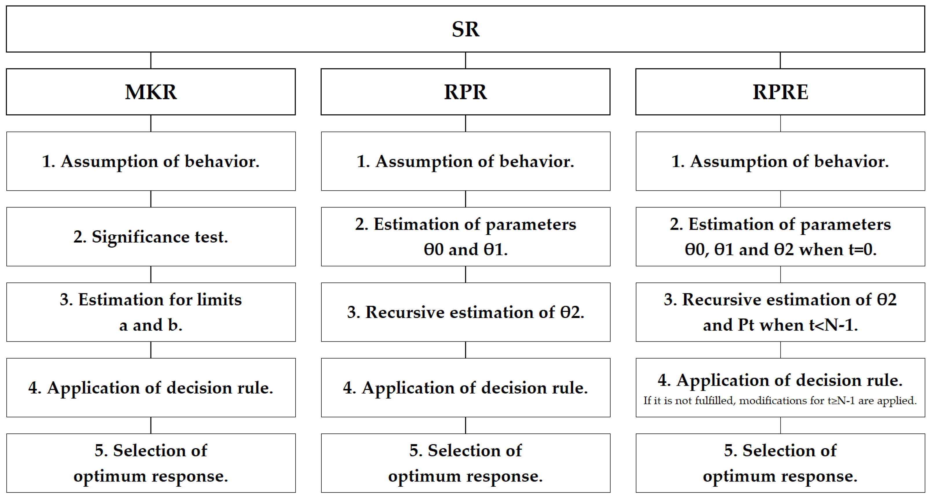
d. Application of MKSR, RPR and RPRE

The intention is to utilize a formal procedure in order to stop at a required value. For this paper, the MKSR, RPR and RPRE will be applied for comparison.

The procedure of Myers and Khuri [17] is as follows:

1. The MKSR assumes the behavior in the observed response $y\left(t\right)$ to be normally distributed; thus $y\left(t\right)\sim normal(\eta \left(t\right),\sigma {}^2)$;

2. A significance test is run using confidence intervals as follows:

$y(n_i+1)-y\left(n_i\right)\ge b$; where individual experimentation continues;

$y(n_i+1)-y\left(n_i\right)<b>a$; where individual experimentation continues;

$y(n_i+1)-y\left(n_i\right)\le a$; where individual experimentation stops;

3. A solution is established for the limits of the procedures a and $-b$ in (2) as follows:

$$a=-b={\mathsf{\Phi }}^{-1}(\frac{1}{2k})\left({\sigma }_{\epsilon }\right)\left(\sqrt{2}\right);$$

(2)

where a and b work as the limits of the interval for the significance test, $\mathsf{\Phi }$ is the normal cumulative distribution function, $\kappa$ is a guess of the number of individual experimentation runs to arrive to the improvement and $\sigma$ is the square root of the adjusted mean square of ANOVA from the factorial analysis;

4. Once the values for a and b are computed, the decision to stop is determined with (3) as follows:

$$y\left(n_i\right)-y\left(n_i-1\right)\le a<0$$

(3)

where $y\left(n_i\right)$ is a present value from the response variables in the path of improvement from SADM, $y(n_i-1)$ is a past value from the path and a is a limit of the interval of the significance test of the procedure;

5. The moment where individual experimentation stopped is the time where the response is considered to be the best. Nevertheless, if a better response is identified in a previous time, that value is the new best response.

On the other hand, ref. [18] presents the RPR procedure:

1. It assumes the behavior of the observed response $y\left(t\right)$ to be quadratic and proposes to obtain the first derivative of $y\left(t\right)=\eta \left(t\right)+{ϵ}_t={\theta }_0+{\theta }_{1}t+{\theta }_2{t}^2+{ϵ}_t$ to obtain $y^{\prime }\left(t\right)={\theta }_1+2{\theta }_{2}t=0$; thus $t^{*}=-{\theta }_1/2{\theta }_2$;

2. The parameters ${\theta }_0$ or $y\left(0\right)$, ${\theta }_1$ and ${\theta }_2$ are estimated as follows:

a. ${\theta }_0$ is obtained by computing the arithmetic mean of center points of the experiment;

b. ${\theta }_1$ is estimated by calculating (4):

$${\theta }_1=\sqrt{b_1{}^2+b_2{}^2+\cdots +b_k{}^2}$$

(4)

where ${\theta }_1$ is one of the parameter estimations that assists computation in the procedure and $bi$ represent the regression coefficients of the linear model;

c. ${\theta }_2$ must be recursively estimated. Therefore, there will be one ${\theta }_2$ for each iteration or individual experimentation t. This means the estimation of ${\theta }_2{}^{\left(t\right)}$;

3. ${\theta }_2{}^{\left(t\right)}$ should be estimated as follows:

a. For ${\theta }_2{}^{\left(0\right)}$, (5) is considered:

$${\theta }_2^{\left(0\right)}=\frac{-{\theta }_1}{2\ast t_{prior}}$$

(5)

where ${\theta }_2^{\left(0\right)}$ works as an estimation for the procedure when $t=0$, and $t_{prior}$ works as an initial guess about the number of iterations or individual experiments that are considered to be necessary to reach the optimum value;

b. For ${\theta }_2{}^{\left(t\right)}$ starting from ${\theta }_2{}^{\left(1\right)}$, the updating is calculated using (6) as follows:

$${\theta }_2^{\left(t\right)}={\theta }_2^{(t-1)}+\frac{P_{t-1}\ast t^2}{1+(t^4\ast P_{t-1})}\ast (Y\left(t\right)-Y\left(0\right)-{\theta }_{1}t-{\theta }_2^{(t-1)}\ast t^2)$$

(6)

where $Y\left(t\right)$ represents the response variable in t time in the path of improvement.

c. To calculate $P_0$ in $P_t$, Miró-Quesada and Del Castillo [18] propose that it is necessary to establish an initial value, similar to the initial guess of $t_{prior}$;

d. For $P_t$ starting from $P_1$, the updating is calculated using (7), as shown next:

$$P_t=(1-\frac{P_{t-1}\ast t^4}{1+t^4\ast P_{t-1}})\ast P_{t-1}$$

(7)

where $P_t$ is considered the scaled variance of ${\theta }_2^{\left(t\right)}$ after t iterations of individual experimentation, noted as: $P_t=\frac{1}{{\sigma }_{ϵ}^2}Var({\theta }_2^{\left(t\right)})$;

e. An estimation for the variance of the error $\left({\sigma }_{({\theta }_1+2{\theta }_2^{\left(t\right)}t)}^2\right)$ is obtained with (8) as follows:

$${\sigma }_{({\theta }_1+2{\theta }_2^{\left(t\right)}t)}^2=4{\sigma }_{ϵ}^2\ast t^2\ast P_t.$$

(8)

This result will be used next for comparison purposes;

4. A decision rule is applied to state if (9) is fulfilled. If so, individual experimentation stops. The in-equation is as follows:

$${\theta }_1+2{\theta }_2^{\left(t\right)}t<-3\sqrt{{\sigma }_{{\theta }_1+2{\theta }_2^{\left(t\right)}t}^2}.$$

(9)

The intention is to compare both sides of (9) to assure the stopping iteration;

5. The iteration where t stopped is the value in y where the response is considered to be the best answer. Nevertheless, if a better response is identified in a previous time, that value is the new best response (the same as in the MKSR).

Finally, Del Castillo [19] explains the RPRE, which recursively fits the intercept and the first-order term in addition to the second-order term in (10), as shown here:

$$Y\left(t\right)=\eta \left(t\right)+{ϵ}_t={\theta }_0+{\theta }_{1}t+{\theta }_2{t}^2+{ϵ}_t$$

(10)

where $\eta \left(t\right)$ denotes the operation ${\theta }_0+{\theta }_{1}t+{\theta }_2{t}^2$.

The procedure can be summarized with the following five main steps:

1. The recursive fitting increases the robustness for non-quadratic behavior by specifying a maximum number of experiments in the recursive least squares algorithm, applying a concept called “window” to fit only a local parabolic model along the search direction to make it less sensitive to large scale deviations from quadratic behavior. The “window” size $\left(N\right)$ is determined using an indicator called “Signal-to-Noise Ratio” (SNR) estimated with (11) as follows:

$$SNR=\frac{∥b∥}{{\sigma }_{ϵ}}$$

(11)

where ${\sigma }_{ϵ}$ is the standard deviation from the center points of the experiment.

The variable $∥b∥$ is estimated using (12) as follows:

$$∥b∥=∥\beta ∥=\sqrt{\sum _{i=1}^k{b}_i^2}.$$

(12)

Finally, it is necessary to identify N in a table of values of window sizes. In the enhanced stopping rule, it is proposed to visualize the $N\times 1$ vector $bN$ and the scalar $\sqrt{vN}$;

2. As in the procedure for the RPR, $t_{prior}$ continues to be an initial guess about the number of individual experiments that are suggested to be necessary to reach the optimum value. Now, for the estimation of parameters when $t=0$, computations (13)–(15) are suggested, as illustrated next:

$${\theta }_0^{\left(0\right)}=Y\left(0\right)$$

(13)

where $Y\left(0\right)$ represents the average of the response variables obtained from the center points of the experiment. Furthermore:

$${\theta }_1^{\left(0\right)}=∥b∥$$

(14)

where $∥b∥$ represents the square root of the sum of the squares of the regression coefficients of the linear model of the experiment. Next:

$${\theta }_2^{\left(0\right)}=-\frac{{\theta }_1^{\left(0\right)}}{2\ast t_{prior}}$$

(15)

where the constant 2 proposed by the author of the rule has the intention of making the value of $t_{prior}$ more robust;

3. The algorithm makes use of the matrix definitions (16)–(19) for updating the three parameters ${\theta }_0$, ${\theta }_1$ and ${\theta }_2$:

$${\theta }^{\left(t\right)}=\left[\begin{array}{c}{\theta }_0^{\left(t\right)}\\ {\theta }_1^{\left(t\right)}\\ {\theta }_2^{\left(t\right)}\end{array}\right];$$

(16)

$${\varphi }_t=\left[\begin{array}{c}1\\ t\\ t^2\end{array}\right];$$

(17)

$$\frac{d{\varphi }_t}{dt}\equiv dt=\left[\begin{array}{c}0\\ 1\\ 2t\end{array}\right];$$

(18)

$$P_0=\left[\begin{array}{ccc}1& 0& 0\\ 0& 1& 0\\ 0& 0& 10\end{array}\right].$$

(19)

The large value of 10 given to $P_0$ makes the rule robust against possibly large discrepancies between $t_{prior}$ and $t^{*}$, giving “adaptation” ability to varying curvature.

Now, (20) is used to update ${\theta }^{\left(t\right)}$:

$${\theta }^{\left(t\right)}={\theta }^{(t-1)}+\frac{P_{t-1}{\varphi }_t}{1+{{\varphi }^{\prime }}_t{P}_{t-1}{\varphi }_t}(Y_{\left(t\right)}-{\varphi }_t^{\prime }{\theta }^{(t-1)}).$$

(20)

Furthermore, (21) is used to update $P_t$:

$$P_t=Var({\theta }^{\left(t\right)})/{\sigma }_{ϵ}^2=(I-\frac{P_{t-1}{\varphi }_t}{1+{\varphi }_t^{\prime }{P}_{t-1}{\varphi }_t}{\varphi }_t^{\prime })P_{t-1};$$

(21)

4. If (22) is fulfilled, the search stops and returns to $t^{*}$, such that the maximum response is determined by $Y\left(t^{*}\right)={max}_{l=1,\dots ,t}\left\{Y\right(l\left)\right\}$. The rule is shown next:

$$d_t^{\prime }{\theta }^{\left(t\right)}<-1.645{\sigma }_{ϵ}\sqrt{d_t^{\prime }{P}_t{d}_t}$$

(22)

where −1.645 represents a standardized value of the normal distribution for a significance level of 0.05.

Otherwise, the procedure continues computing $t\ge N-1$ following the next steps according to Del Castillo [19]:

a. Perform an experiment at step $t\ge N-1$;

b. Update vector $Y_N\left(t\right)$ with the observed value $Y_{\left(t\right)}$ by discarding its first element, shifting the remaining elements one position up in the vector and including $Y\left(t\right)$ as the last element in $Y_N\left(t\right)$;

c. Read $b_N$ and $v_N$ using the table of values of window size N in the enhanced stopping rule proposed by [19], where it is possible to visualize the $N\times 1$ vector $bN$ and the scalar $\sqrt{v_N}$. After this, continue individual experimentation until (23) is fulfilled:

$$b_N^{\prime }{Y}_N\left(t\right)<-1.645{\sigma }_{ϵ}\sqrt{v_N};$$

(23)

5. If the inequality holds, then stop the search and return $t^{*}$ such that $Y\left(t^{*}\right)={max}_{l=1,\dots ,t}\left\{Y\right(l\left)\right\}$.

Next, Figure 2 shows the steps to follow in each of the SRs previously mentioned.

e. Selection of the rule with best performance for each case.

In this last stage of the method, the response value with the best performance is observed for each of the simulators. This means that through the analysis, either the MKSR, RPR or RPRE will have better performance according to the application of each SR and their adjustment with the behavior of the data. For each simulator, the best value and SR is mentioned.

3. Results

The analysis considers two cases. The selection of these two simulated cases is based on the importance of a well-performed approach to processes with several inputs and only one output. The combination of levels and factors is vital to understanding the interactions in the system; nonetheless, identifying relevant factors even among several of them is indispensable in terms of optimization of the response. Furthermore, as multiple experiments are required for the comparison of the considered stopping rules, the simulated processes may represent an important option, as they offer practical scenarios that can be reproducible for optimization purposes. These two cases follow factorial designs, which contain seven factors, two levels, six center points and two replicates. This gives a total of 262 experimental runs per case. The first case has factors $P,Q,R,S,T,U$ and V. The low levels for each of these factors are 11, 68, 67, 275, 0.4, 70 and 16, respectively. The high levels for the factors are 13.5, 84, 92, 300, 0.5, 80 and 20, respectively. After the factorial analysis was performed using Minitab^®, only factors $P,Q,S$ and U were significant for the response. The second case has factors $S,T,Y,Z,E,F$ and G. The low levels for each of these factors are 325, 650, −2, 1.4, 1, 28.5 and 9, respectively. The high levels for these factors are 350, 700, 0, 1.5, 3.0, 31 and 13, respectively. Only factors $Y,Z,E$ and G were significant. This information was used in both cases to build the steepest path using the procedure in [13] to determine the step size of the path for each of the significant factors. The sufficiency of diversity in the nature of these experiments to generalize findings and make more general recommendations will follow the conditions and properties of the experiment itself. This means that all conclusions will be highly valuable for oncoming situations with similar natures and characteristics to the ones here presented.

Next, the application of the three mentioned SRs in Case 1.

3.1. Results for Case 1

The coded unit regression equation for Case 1 is:

$y=4.2943-0.0367P+0.2123Q-0.0381S+0.0519U$.

The path for the steepest ascent is built considering:

• The selection of a step size for this path. The variable with the largest absolute regression coefficient is the one selected. In this case, factor Q is selected;
• The proposed natural step size for the factor Q is ${\Delta }_Q=1$. Through conversion from coded to natural units, the coded step size for Q is ${\Delta }_{X_Q}=0.1250$;
• The calculation of the coded step sizes for the rest of the variables is performed with (1).
  For example, the coded step size of P is:
  ${\Delta }_{X_P}=\frac{-0.0367}{0.2123/0.1250}=-0.0216.$
  Thus, the coded step sizes for the significant factors are:
  ${\Delta }_{X_P}=-0.0216$ for P,
  ${\Delta }_{X_Q}=0.1250$ for Q,
  ${\Delta }_{X_S}=-0.0224$ for S and;
  ${\Delta }_{X_U}=0.0306$ for U.
  The natural step sizes for the same factors are:
  ${\Delta }_P=-0.0270$ for P,
  ${\Delta }_Q=1$ for Q,
  ${\Delta }_S=-0.2804$ for S and;
  ${\Delta }_U=5$ for U.
  The path for Case 1 is built next.

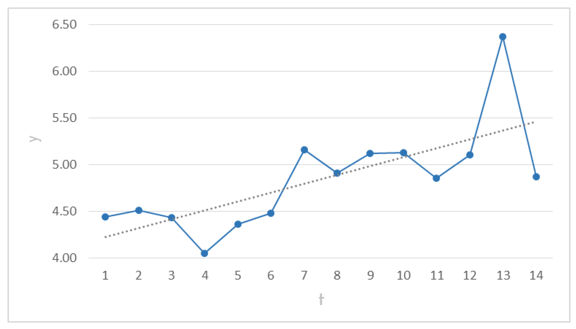
Application of MKSR to Case 1

1. Assumption of behavior in Case 1. The steepest direction is shown in

Table 1. Implementation of steepest ascent path for Case 1.

t	P	Q	S	U	y
0	12.30	76.00	287.50	75.00	4.62
1	12.20	77.00	287.20	80.00	4.44
2	12.20	78.00	286.90	85.00	4.51
3	12.20	79.00	286.70	90.00	4.43
4	12.10	80.00	286.40	95.00	4.05
5	12.10	81.00	286.10	100.00	4.36
6	12.10	82.00	285.80	105.00	4.48
7	12.10	83.00	285.50	110.00	5.16
8	12.00	84.00	285.30	115.00	4.91
9	12.00	85.00	285.00	120.00	5.12
10	12.00	86.00	284.70	125.00	5.13
11	12.00	87.00	284.40	130.00	4.85
12	11.90	88.00	284.10	135.00	5.10
13	11.90	89.00	283.90	140.00	6.37
14	11.90	90.00	283.60	145.00	4.87

, running 15 iterations. It starts with step 0, computing the center points of the experiment.

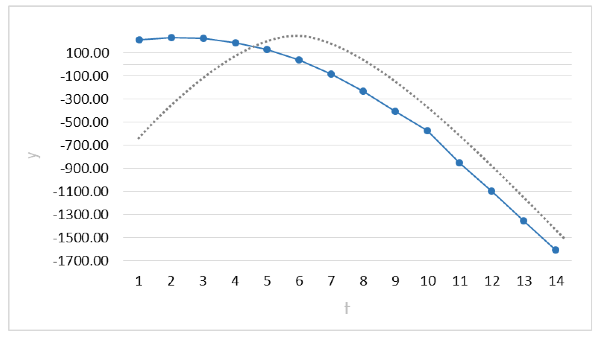
This procedure assumes a normally distributed behavior in response $y\left(t\right)$. Figure 3 shows the behavior of the response in its steepest path from $t=1$ to $t=14$. The straight line tries to illustrate the assumption of normality for the response.

2. Significance test in Case 1. Iterations or individual experimentation through the steepest path stop when $y(n_i+1)-y\left(n_i\right)\le a$.

3. Estimation for limits a and b in Case 1. Limits $a=-0.744$ and $-b=0.744$ are calculated using (2) as shown in

Table 2. Obtained limits of MKR in Case 1.

a	b	${\mathsf{\Phi }}^{-1}\left(1/2\mathit{k}\right)$	${\mathit{\sigma }}_{\mathit{ϵ}}$	$\sqrt{2}$
−0.74	0.74	−1.83	0.28	1.41

. Those limits are used to identify the moment where (3) is fulfilled. It is important to remember that the value of $\kappa$ is a guess of the number of individual experimentation runs to arrive at the improvement. In this case, the considered value of $\kappa =15$.

4. Application of decision rule in Case 1. The decision to stop is determined by (3). This means that the time t should stop when $y\left(n_i\right)-y\left(n_i-1\right)\le -0.744$. The behavior of the data is shown in

Table 3. Obtained results from MKSR procedure in Case 1.

t	P	Q	S	U	y	$\mathit{y}({\mathit{n}}_{\mathit{i}}+1)-\mathit{y}\left({\mathit{n}}_{\mathit{i}}\right)$	Status
0	12.30	76.00	287.50	75.00	4.62	-	Starts
1	12.20	77.00	287.20	80.00	4.44	−0.18	Continues
2	12.20	78.00	286.90	85.00	4.51	0.07	Continues
3	12.20	79.00	286.70	90.00	4.43	−0.08	Continues
4	12.10	80.00	286.40	95.00	4.05	−0.38	Continues
5	12.10	81.00	286.10	100.00	4.36	0.31	Continues
6	12.10	82.00	285.80	105.00	4.48	0.12	Continues
7	12.10	83.00	285.50	110.00	5.16	0.68	Continues
8	12.00	84.00	285.30	115.00	4.91	−0.25	Continues
9	12.00	85.00	285.00	120.00	5.12	0.21	Continues
10	12.00	86.00	284.70	125.00	5.13	0.01	Continues
11	12.00	87.00	284.40	130.00	4.85	−0.28	Continues
12	11.90	88.00	284.10	135.00	5.10	0.25	Continues
13	11.90	89.00	283.90	140.00	6.37	1.27	Continues
14	11.90	90.00	283.60	145.00	4.87	−1.50	Stops

.

5. Selection of optimum response in Case 1. If $y\left(n_i\right)-y\left(n_i-1\right)\le a$, the search stops and it returns to $t^{*}$ such that $Y\left(t^{*}\right)={max}_{l=1,\dots ,t}\left\{Y\right(l\left)\right\}.$ As noted, the best performance for the MKSR us found in iteration 13, with a response of 6.37 units.

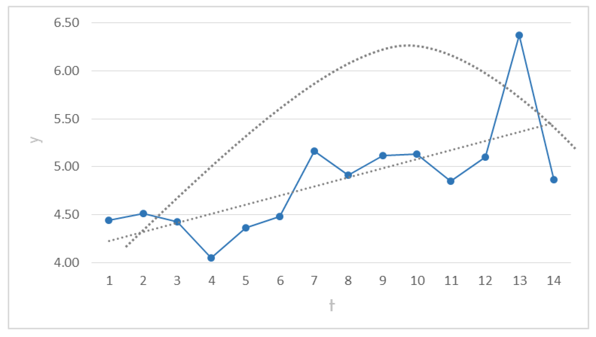
Application of RPR to Case 1

1. Assumption of behavior in Case 1. The steepest path applies the same way for this case. Now, Figure 4 shows the behavior of the response in the steepest path from $t=1$ to $t=14$. The curved line tries to illustrate the quadratic assumption of the response.

2. Estimation of parameters ${\theta }_0$ and ${\theta }_1$ in Case 1. The estimation starts with ${\theta }_0$, which is obtained by calculating the arithmetic mean of center points. In this case:

${\theta }_0=\frac{4.10+4.41+4.42+4.37+3.88+4.45}{6}$; thus, ${\theta }_0=Y\left(0\right)=4.2710$.

Applying (4) through the coefficients of significant factors,

${\theta }_1=\sqrt{{(-0.0367)}^2+{\left(0.2123\right)}^2+{(-0.0381)}^2+{\left(0.0519\right)}^2}=0.2249$.

This is known as the slope of the response function at the origin in the steepest direction.

3. Recursive estimation of parameters in Case 1.

Table 4. Obtained results of the RPR procedure in Case 1.

t	$\mathit{y}\left(\mathit{t}\right)$	${\mathit{\theta }}_2^{\left(\mathit{t}\right)}$	$\mathit{P}\mathit{t}$	${\mathit{\theta }}_1+2{\mathit{\theta }}_2^{\left(\mathit{t}\right)}\mathit{t}$	${\mathit{\sigma }}_{{\mathit{\theta }}_1+2{\mathit{\theta }}_2^{\left(\mathit{t}\right)}\mathit{t}}^2$	$-3\sqrt{{\mathit{\sigma }}_{{\mathit{\theta }}_1+2{\mathit{\theta }}_2^{\left(\mathit{t}\right)}\mathit{t}}^2}$	Status
0	4.62	−0.01	10	0.22	0.00	0.00	Starts
1	4.44	−0.05	0.91	0.12	0.30	−1.64	Continues
2	4.51	−0.05	0.06	0.01	0.08	−0.83	Continues
3	4.43	−0.06	0.01	−0.11	0.03	−0.52	Continues
4	4.05	−0.07	0.00	−0.31	0.01	−0.37	Continues
5	4.36	−0.05	0.00	−0.28	0.00	−0.27	Stops

details the recursive estimation of parameters, which assists the stopping decision. For this case, $P_0=t_{prior}=10.$

4. Application of decision rule in Case 1. The decision to stop is given when (9) is fulfilled. The "Status" column of Table 4 shows the moment that this occurs.

5. Selection of optimum response in Case 1. As seen in Table 8, the decision to stop occurred in iteration 5; nevertheless, the best response was at 4.62 units because it returns to $t^{*}$ such that $Y\left(t^{*}\right)={max}_{l=1,\dots ,t}\left\{Y\right(l\left)\right\}.$

Application of RPRE to Case 1

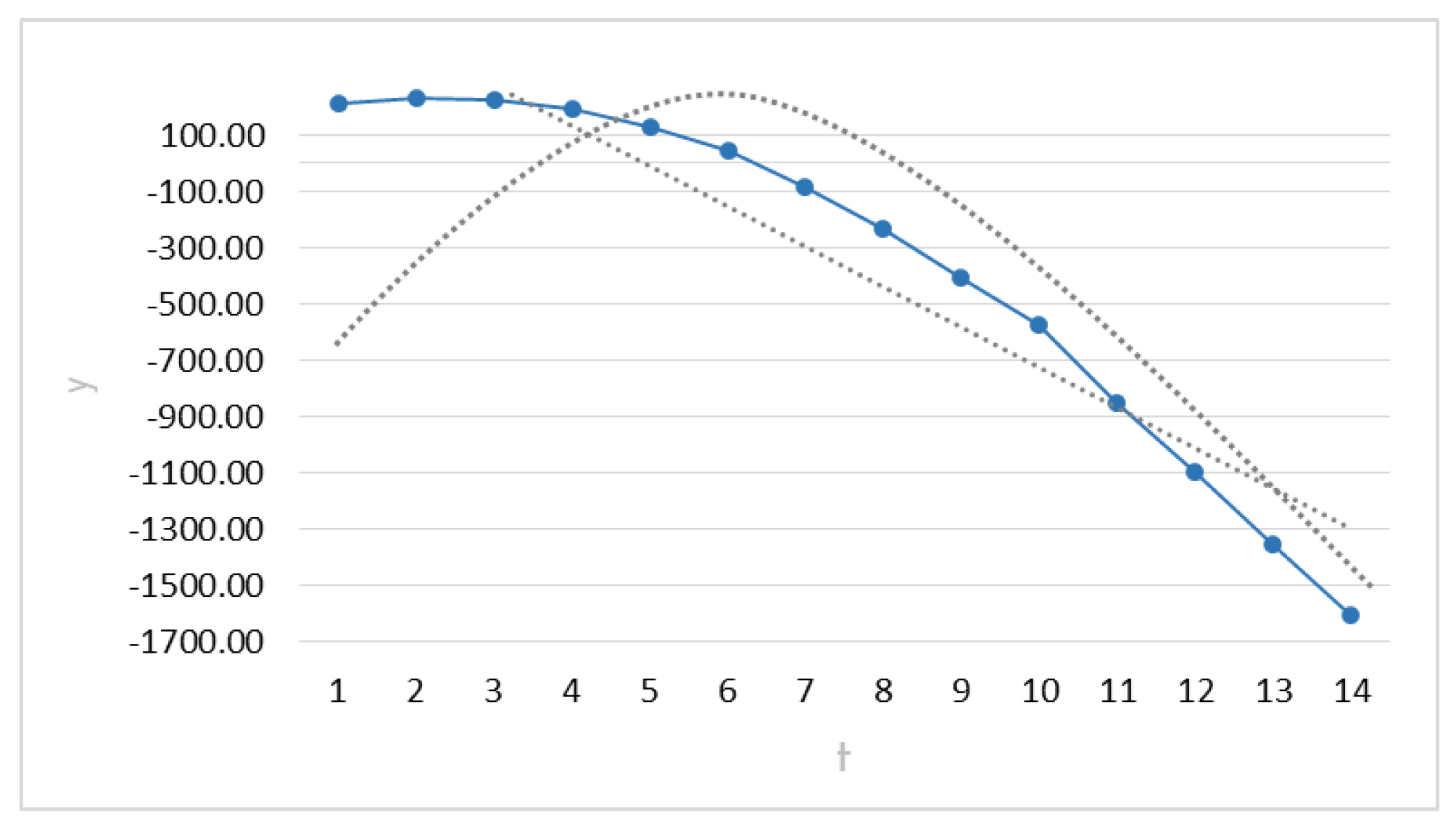
1. Assumption of behavior in Case 1.Figure 5 shows the response behavior in the steepest path and the assumption of both quadratic and non-quadratic behavior. The straight and curved lines illustrate the capability of this procedure to assume both types of behavior.

In order to estimate the indicator SNR and obtain the N, it is necessary to use (12) to compute:

$∥b∥=\sqrt{{\sum }_{i=1}^k\left(b_i^2\right)}=\sqrt{(-{0.04}^2)+{\left(0.21\right)}^2+{(-0.04)}^2+{\left(0.05\right)}^2}=0.22$.

This is the slope of the response function at the origin in the steepest direction.

Then, (11) is applied to estimate the indicator $SNR$:

$SNR=\frac{∥b∥}{{\sigma }_{ϵ}}=\frac{0.22}{0.21}=0.23.$

This indicator makes the value $N=15$. It means that computations shall start for:

$t<N-1\therefore t<15-1\therefore t<14.$

2. Estimation of parameters ${\theta }_0$, ${\theta }_1$ and ${\theta }_2$ when $t=0$ in Case 1.

Results for parameters ${\theta }_0$, ${\theta }_1$ and ${\theta }_2$ when $t=0$ are presented next:

${\theta }_0^{\left(0\right)}=4.62$;   ${\theta }_1^{\left(0\right)}=0.22$;   ${\theta }_2^{\left(0\right)}=-0.01$.

3. Recursive estimation of ${\theta }_2$ and $P_t$ when $t<N-1$ in Case 1.

Table 5. Recursive procedure of ${\theta }_i$ and $P_t$ when $t<N-1$.

t	$\mathit{Y}\left(\mathit{t}\right)$	${\mathit{\theta }}_0$	${\mathit{\theta }}_1$	${\mathit{\theta }}_2$	${\mathit{P}}_{\mathit{t}}$			${\mathit{d}}_{\mathit{t}}^{\prime }{\mathit{\theta }}^{\left(\mathit{t}\right)}$	$-1.645{\mathit{\sigma }}_{\mathit{ϵ}}\sqrt{{\mathit{d}}_{\mathit{t}}^{\prime }{\mathit{P}}_{\mathit{t}}{\mathit{d}}_{\mathit{t}}}$
					1	0	0
0	4.62	4.62	0.23	−0.01	0	1	0	0.23	NA
					0	0	10
					0.90	−0.10	−0.80
1	4.44	4.59	0.19	−0.31	−0.10	0.90	−0.80	−0.43	−0.91
					−0.80	−0.80	2.30
					0.70	−0.20	−0.10
2	4.51	4.51	0.15	−0.08	−0.20	0.90	−0.40	−0.19	−0.53
					−0.10	−0.40	0.30
					0.60	−0.30	0.00
3	4.43	4.49	0.12	−0.05	−0.30	0.70	−0.20	−0.18	−0.38
					0.00	−0.20	0.10
					0.60	−0.30	0.00
4	4.05	4.50	0.14	−0.06	−0.30	0.60	−0.10	−0.28	−0.30
					0.00	−0.10	0.00
					0.60	−0.30	0.00
5	4.36	4.50	0.02	−0.02	−0.30	0.40	−0.10	−0.48	−0.25
					0.00	−0.10	0.00

shows the recursive procedure of ${\theta }_i$ and $P_t$ when $t<N-1$. For this case, $P_0$ obeys (19) and $t_{prior}=18.$

4. Application of decision rule in Case 1. If it is not fulfilled, modifications for $t\ge N-1$ are applied.

In this case, in-equation $d_t^{\prime }{\theta }^{\left(t\right)}<-1.645{\sigma }_{ϵ}\sqrt{d_t^{\prime }{P}_t{d}_t}$ is fulfilled, so the search stops and returns to $t^{*}$, such that $Y\left(t^{*}\right)={max}_{l=1,\dots ,t}\left\{Y\right(l\left)\right\}$.

5. Selection of optimum response in Case 1.Table 5 shows the decision to stop, which occurred in iteration 5. Nevertheless, the best response was at 4.62 units.

Now, the application of the three SRs in Case 2.

3.2. Results for Case 2

The coded unit regression equation for Case 2 is:

$y=149.7810+9.5079Y-0.2023Z+31.1119E+29.8927G$.

The path for the steepest ascent is built considering:

• The selection of a step size for this path. The variable with the largest absolute regression coefficient is the one selected. In this case, factor E is the one selected to propose a natural step size;
• The proposed natural step size for factor E is the unit; thus, the step size for E is $\Delta E=1.0000$. Through conversion from coded to natural units, the coded step size for E is $\Delta X_E=1.0000$. By coincidence, it is equal for both coded and natural units;
• The calculation of coded step size in the other variables is performed with (1). For example, the coded step size of Z is:
  ${\Delta }_{X_Z}=\frac{-0.2023}{31.1119/1.0000}=-0.0065.$
  Thus, the coded step sizes for the significant factors are:
  ${\Delta }_{X_Y}=0.3056$ for Y,
  ${\Delta }_{X_Z}=-0.0065$ for Z,
  ${\Delta }_{X_E}=1.0000$ for E and;
  ${\Delta }_{X_G}=0.9608$ for G.
  The natural step sizes for the same factors are:
  ${\Delta }_Y=0.3056$ for Y,
  ${\Delta }_Z=-0.0003$ for Z,
  ${\Delta }_E=1.0000$ for E and;
  ${\Delta }_G=1.9216$ for G.

The path for Case 2 can now be built.

Application of MKSR to Case 2

1. Assumption of behavior in Case 2.

Table 6. Obtained results for the steepest ascent path of Case 2.

t	Y	Z	E	G	y
0	−1.00	1.50	2.00	11.00	163.41
1	−0.70	1.40	3.00	12.90	212.22
2	−0.40	1.40	4.00	14.80	232.75
3	−0.10	1.40	5.00	16.80	226.16
4	0.20	1.40	6.00	18.70	191.12
5	0.50	1.40	7.00	20.60	130.32
6	0.80	1.40	8.00	22.50	42.51
7	1.10	1.40	9.00	24.50	−82.49
8	1.40	1.40	10.00	26.40	−233.67
9	1.80	1.40	11.00	28.30	−405.47
10	2.10	1.40	12.00	30.20	−573.87
11	2.40	1.40	13.00	32.10	−849.67
12	2.70	1.40	14.00	34.10	−1094.76
13	3.00	1.40	15.00	36.00	−1356.20
14	3.30	1.40	16.00	37.90	−1605.82

shows the steepest path from iteration 0 to 14.

Next, Figure 6 shows the behavior of the response in its steepest path from $t=1$ to $t=14$.

2. Significance test in Case 2. As in Case 1, individual experimentation over the steepest path stops when $y(n_i+1)-y\left(n_i\right)\le a$.

3. Estimation for limits a and b in Case 2. Limits $a=-3.668$ and $b=3.668$ are calculated using (2) with $\kappa =30$, as shown in

Table 7. Obtained limits of the MKSR in Case 2.

a	b	${\mathsf{\Phi }}^{-1}\left(1/2\mathit{k}\right)$	${\mathit{\sigma }}_{\mathit{ϵ}}$	$\sqrt{2}$
−3.67	3.67	−1.83	1.41	1.41

. Those limits are used to identify the moment where (3) is fulfilled.

4. Application of decision rule in Case 2. The decision to stop occurs when

$y\left(n_i\right)-y\left(n_i-1\right)\le -3.67$. The behavior is shown in

Table 8. Results for the MKSR procedure in Case 2.

t	Y	Z	E	G	y	$\mathit{y}(\mathit{ni}+1)-\mathit{y}\left(\mathit{ni}\right)$	Status
0	−1.00	1.50	2.00	11.00	163.41	-	Starts
1	−0.70	1.40	3.00	12.90	212.22	48.81	Continues
2	−0.40	1.40	4.00	14.80	232.75	20.54	Continues
3	−0.10	1.40	5.00	16.80	226.16	−6.60	Stops

.

5. Selection of optimum response in Case 2. In this case, the best performance for the MKSR in Case 2 is the response of 232.75 units, because it stopped in $t^{*}$ such that $Y\left(t^{*}\right)={max}_{l=1,\dots ,t}\left\{Y\right(l\left)\right\}.$

Application of RPR to Case 2

1. Assumption of behavior in Case 2. Figure 7 shows behavior of the response in the steepest path.

2. Estimation of parameters ${\theta }_0$ and ${\theta }_1$ in Case 2. These estimations are shown next:

${\theta }_0=\frac{163.23+162.70+162.44+162.02+162.67+163.22}{6}=Y\left(0\right)=162.71$.

This next estimation is performed the same way as in the previous case (Case 1):

${\theta }_1=\sqrt{\left(9.5079\right){}^2+(-0.2023){}^2+\left(31.1119\right){}^2+\left(29.8927\right){}^2}=44.18$.

3. Recursive estimation of parameters in Case 2.

Table 9. Obtained results for the RPR procedure in Case 2.

t	$\mathit{y}\left(\mathit{t}\right)$	${\mathit{\theta }}_2^{\left(\mathit{t}\right)}$	$\mathit{Pt}$	${\mathit{\theta }}_1+2{\mathit{\theta }}_2^{\left(\mathit{t}\right)}\mathit{t}$	${\mathit{\sigma }}_{{\mathit{\theta }}_1+2{\mathit{\theta }}_2^{\left(\mathit{t}\right)}\mathit{t}}^2$	$-3\sqrt{{\mathit{\sigma }}_{{\mathit{\theta }}_1+2{\mathit{\theta }}_2^{\left(\mathit{t}\right)}\mathit{t}}^2}$	Status
0	163.41	−2.21	10.00	44.18	0.00	0.00	Starts
1	212.22	4.64	0.91	53.46	7.27	−8.09	Continues
2	232.75	−3.99	0.06	28.23	1.87	−4.10	Continues
3	226.16	−7.03	0.01	1.98	0.73	−2.57	Continues
4	191.12	−8.65	0.00	−25.02	0.36	−1.80	Stops

shows the recursive estimation needed with $P_0=t_{prior}=10.$

4. Application of decision rule in Case 2. The “Status” column in Table 9 shows the moment when (9) is fulfilled.

5. Selection of optimum response in Case 2. Table 11 illustrates the decision to stop, which occurred in iteration 4. However, the selection falls in $t^{*}$ such that $Y\left(t^{*}\right)={max}_{l=1,\dots ,t}\left\{Y\right(l\left)\right\}$; therefore, the best response was at 232.75 units.

Application of RPRE to Case 2

1. Assumption of behavior in Case 2.Figure 8 shows the behavior of the response in the steepest path and the assumption of both quadratic and linear behavior.

The variable $∥b∥=44.181$.

The indicator $STNR=95.005$.

This makes the value of $N=3$.

This means that computations shall start for $t<N-1\therefore t<3-1\therefore t<2.$

2. Estimation of parameters ${\theta }_0$, ${\theta }_1$ and ${\theta }_2$ when $t=0$ in Case 2.

Results for parameters ${\theta }_0$, ${\theta }_1$ and ${\theta }_2$ when $t=0$ are presented next:

${\theta }_0^{\left(0\right)}=163.4100$;   ${\theta }_1^{\left(0\right)}=44.1810$;   ${\theta }_2^{\left(0\right)}=-2.2091$.

3. Recursive estimation of ${\theta }_2$ and $P_t$ when $t<N-1$ in Case 2.

Table 10. Recursive procedure of ${\theta }_i$ and $P_t$ when $t<N-1$.

t	$\mathit{y}\left(\mathit{t}\right)$	${\mathit{\theta }}_0$	${\mathit{\theta }}_1$	${\mathit{\theta }}_2$	${\mathit{P}}_{\mathit{t}}$			${\mathit{d}}_{\mathit{t}}^{\prime }{\mathit{\theta }}^{\left(\mathit{t}\right)}$	$-1.645{\mathit{\sigma }}_{\mathit{ϵ}}\sqrt{{\mathit{d}}_{\mathit{t}}^{\prime }{\mathit{P}}_{\mathit{t}}{\mathit{d}}_{\mathit{t}}}$
					1	0	0
0	163.41	163.41	44.18	−2.21	0	1	0	44.18	−0.70
					0	0	10
					0.90	−0.10	−0.80
1	212.22	163.94	44.71	3.05	−0.10	0.90	−0.80	50.80	−1.86
					−0.80	−0.80	2.30

shows the recursive procedure of ${\theta }_i$ and $P_t$ when $t<N-1$.

$P_0$ follows (19) and $t_{prior}=10.$

4. Application of decision rule in Case 2. If it is not fulfilled, modifications for $t\ge N-1$ are applied.

In this case, in-equation $d_t^{\prime }{\theta }^{\left(t\right)}<-1.645{\sigma }_{ϵ}\sqrt{d_t^{\prime }{P}_t{d}_t}$ is not fulfilled, so the search continues for $t\ge N-1$, as seen in

Table 11. Recursive procedure for $t\ge N-1$.

t	$\mathit{Y}\left(\mathit{t}\right)$		$\mathit{YN}\left(\mathit{t}\right)$		${\mathit{b}}^{\prime }\mathit{NYN}\left(\mathit{t}\right)$	$-1.645{\mathit{\sigma }}_{\mathit{ϵ}}\sqrt{\mathit{vN}}$
2	232.75	163.41	212.22	232.75	6.40	−1.78
3	226.16	212.22	232.75	226.16	−20.16	−1.78

.

5. Selection of optimum response in Case 2.Table 11 shows the decision to stop, which occurred in iteration 3. Nevertheless, the best response was at 232.75 units due to $t^{*}$ in $Y\left(t^{*}\right)={max}_{l=1,\dots ,t}\left\{Y\right(l\left)\right\}.$

4. Discussion

Now that the three SR procedures have been applied for both cases, the discussion and comparison of the best performance are presented next. In Case 1, the method from [17] needed 14 iterations to stop, giving an optimum response of 6.37. The method from [18] stopped at the fifth iteration, obtaining the optimum response of 4.62. The method from [19] had the same results as the previous one. In Case 2, Ref. [17] needed 3 iterations to stop, delivering a response of 232.75. Ref. [18] stopped at the fourth iteration, with 232.75 as a response. Ref. [19] obtained 232.75 after 3 iterations. The most important piece of information in this case is related to the maximized shown response. For these cases, the number of iterations is not as critical as the response obtained, due to the adaptation that it could suffer. This means that the higher the step size for the steepest path, the faster the maximum response will be reached. However, the intention is to carefully analyze the experiment and the obtained outcomes for comparison.

Table 12. Performance comparison for the three SRs.

Author and Year of SR Procedure	Case 1		Case 2
	Iterations to Stop	Best Response	Iterations to Stop	Best Response
R. Myers and Khuri (1979) MKSR	14	6.37	3	232.75
Miró-Quezada and Del Castillo (2004) RPR	5	4.62	4	232.75
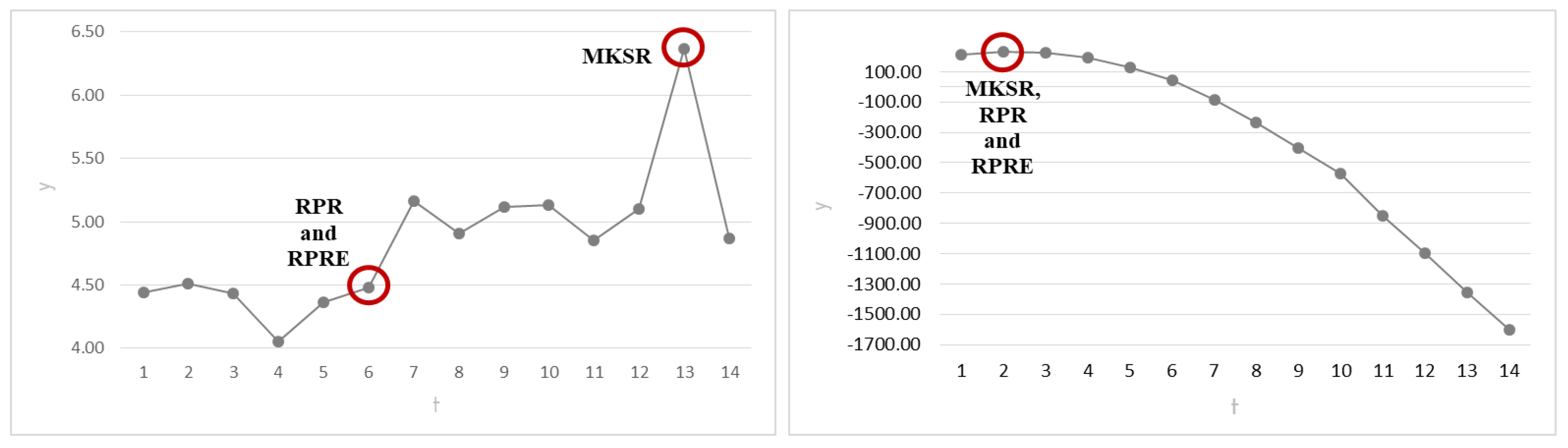
Del Castillo (2007) RPRE	5	4.62	3	232.75

illustrates information of the results. Furthermore, Figure 9 shows the best results for each of the two analyzed cases.

The behavior of the responses of the individual experiments in both study cases is considerably different. In the graph on the right side of Figure 9, the shape of the response tends to resemble a simple parametric function, which could be compared to a quadratic or even a logarithmic model. In these functions, it is relatively easy to find a maximum or a minimum point. This situation becomes evident when observing the way in which the three SRs determined the maximum point in the same place. However, the issue becomes complicated by a case such as the graph on the left side of Figure 9, in which the response does not follow a fixed trend. On the contrary, it shows random variations up and down, so it cannot easily be assimilated into a specific behavior. When this occurs, it can be said that this is a case belonging to a stochastic model. An interesting phenomenon occurs in this type of behavior; the performances of the SRs are not the same; they does not coincide and are different from one another. In a few words, the evidence shown here suggests that the performances of the SRs are similar when the response obeys a parametric function. On the other hand, the performances of the SRs differ when the response exhibits stochastic behavior.

In the particular case of this analysis and under the conditions proposed, the MKSR seems to have better performance, while it is observed that the RPR and the RPRE show a lower output. This situation is not strange; it is explained due to the assumptions of each rule. The MKSR assumes normally distributed behavior, the RPR suggests a quadratic parametric function, and the RPRE obeys quadratic and non-quadratic behavior. None of the previous assumptions easily adjusted to the responses of these individual experiments; however, the MKSR adjusted to give a higher performance.

As previously mentioned, an important task here was to conduct experimentation to simulate behaviors for these three applied stopping procedures. This allowed the possibility of comparison and selection of the procedure with the best performance. The results, with responses and number of needed iterations, are visualized above.

At this point, the complexity of the behavior of the trajectory is particularly important, because it becomes necessary to not only infer using parametric known functions, but also to consider the analysis of these stochastic behaviors. Fortunately, there are several stochastic models that can be considered to characterize the behavior of a steepest ascent trajectory. The Wiener process may be a good option, as it has non-monotone increments with a drift and diffusion parameters that can characterize the randomness in a trajectory, which is the case of the steepest ascent. Stopping rules can be implemented in the stochastic process by considering specific parametric functions in the drift to define a recursive strategy to determine the stopping time.

5. Conclusions

As mentioned by [21], several industrial activities follow Research and Development (R&D) schemes to develop new products or to improve existing ones by analyzing different factorial designs, considering the results of experimentation obtained with repetitions, preliminary results and deviations. The main goal is the response improvement seen as the process of obtaining the optimum result of experimentation on an initially constructed optimization strategy by applying different methods, procedures or rules.

In this case, the applied procedures were DOE, SADM and, finally, three SRs (MKSR, RPR and RPRE). The first of these, the MKSR, assumes normality in the data. This means that linear behavior is the core for the data analysis. On the other hand, the RPR considers parabolic behavior in the information. This means that a quadratic function takes place for this procedure. However, it is reported that the RPRE is as robust, as it is able to work properly with normality, non-normality, quadratic and non-quadratic behavior.

The nature and conditions of the case study and experiment developed will always be critical for the development of each of the procedure and rules. In this case, the conditions related to the designed experiment considered a full factorial design with seven factors, two levels, six center points and two replicates. This gives a total of 262 experimental runs per case. The analysis of this factorial design produced the lineal equation of coded units as the core piece of information for the steepest path. Once the path was built, the decision to stop was critical, because it determined the efficiency of the applied stopping procedure.

The aim was to maximize the response; other schemes of experimentation should be proposed if the intention is to minimize the response or if the researchers wish to obtain a certain value. The SRs illustrated assumed a certain and specific parametric function to establish their theoretical base.

Considering this, and as previously mentioned, research shall continue to propose new exploration schemes relating stochastic processes with the possibility of modifying the parametric base to better characterize the random behavior of the improvement trajectory, in order to search for minimum, maximum or target values.