
GPU Based Modelling and Analysis for Parallel Fractional Order Derivative Model of the Spiral-Plate Heat Exchanger


Abstract
1. Introduction
2. Preliminaries and Problem Statement
2.1. Parallel Fractional Order Derivative Model
2.2. Problem Statement
3. Mathematics Analysis
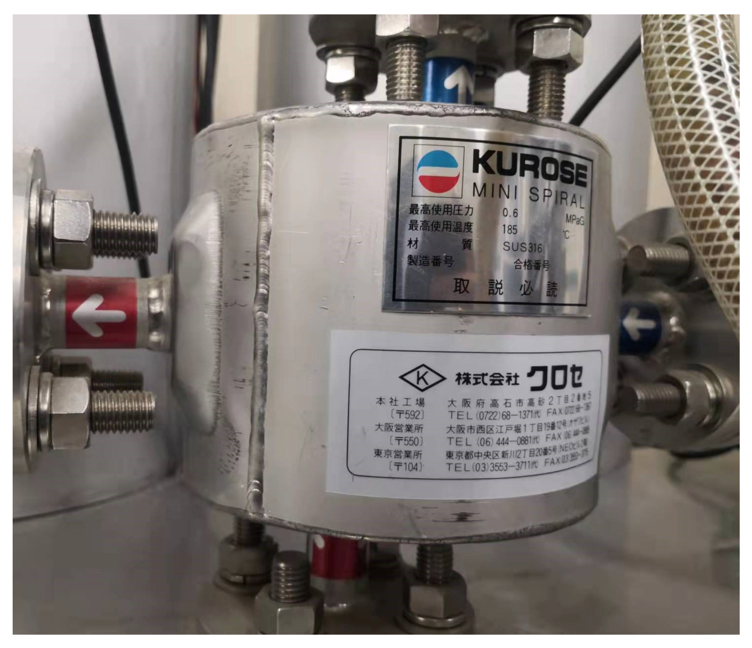
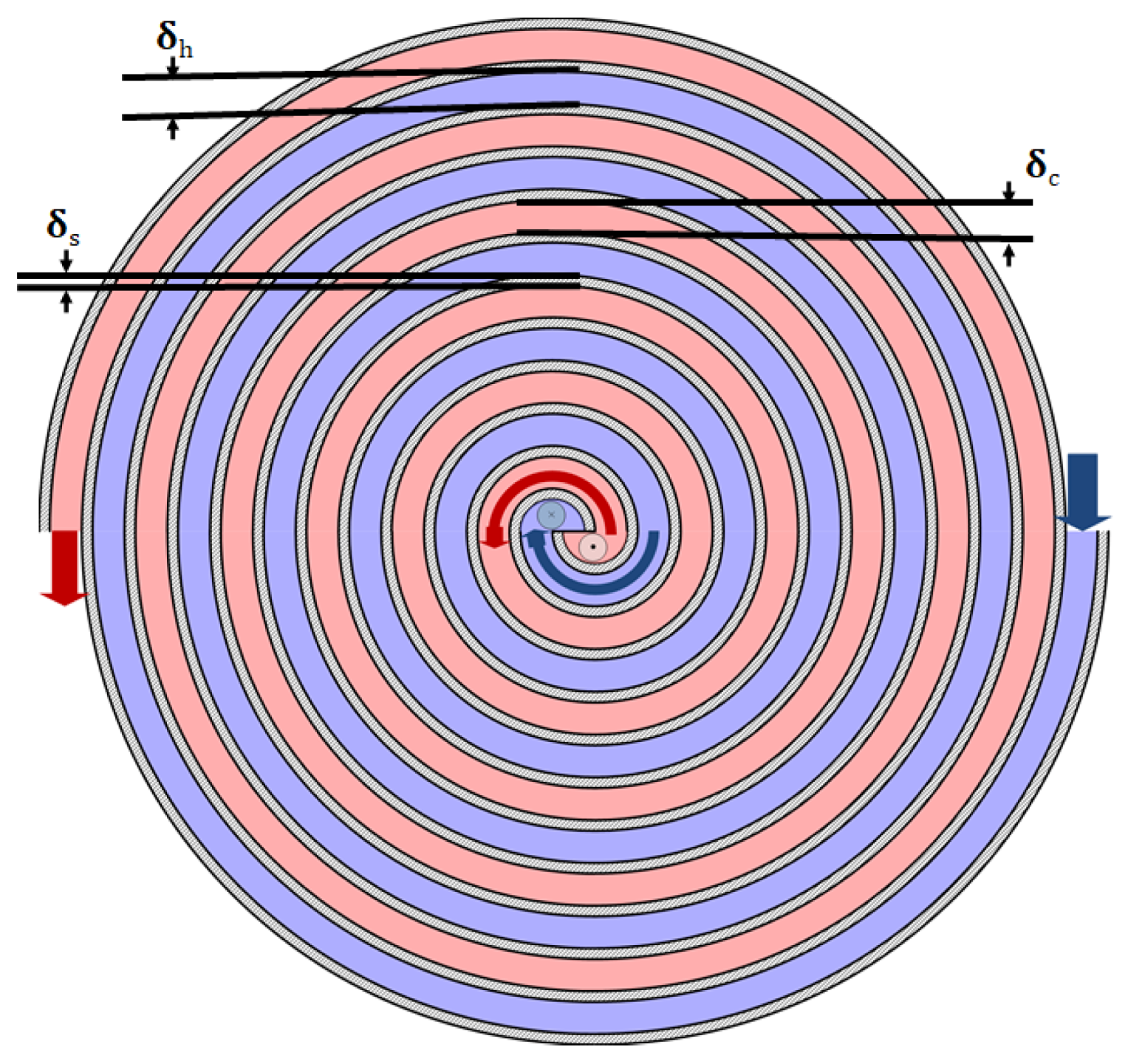
3.1. A Spiral-Plate Heat Exchanger Plant
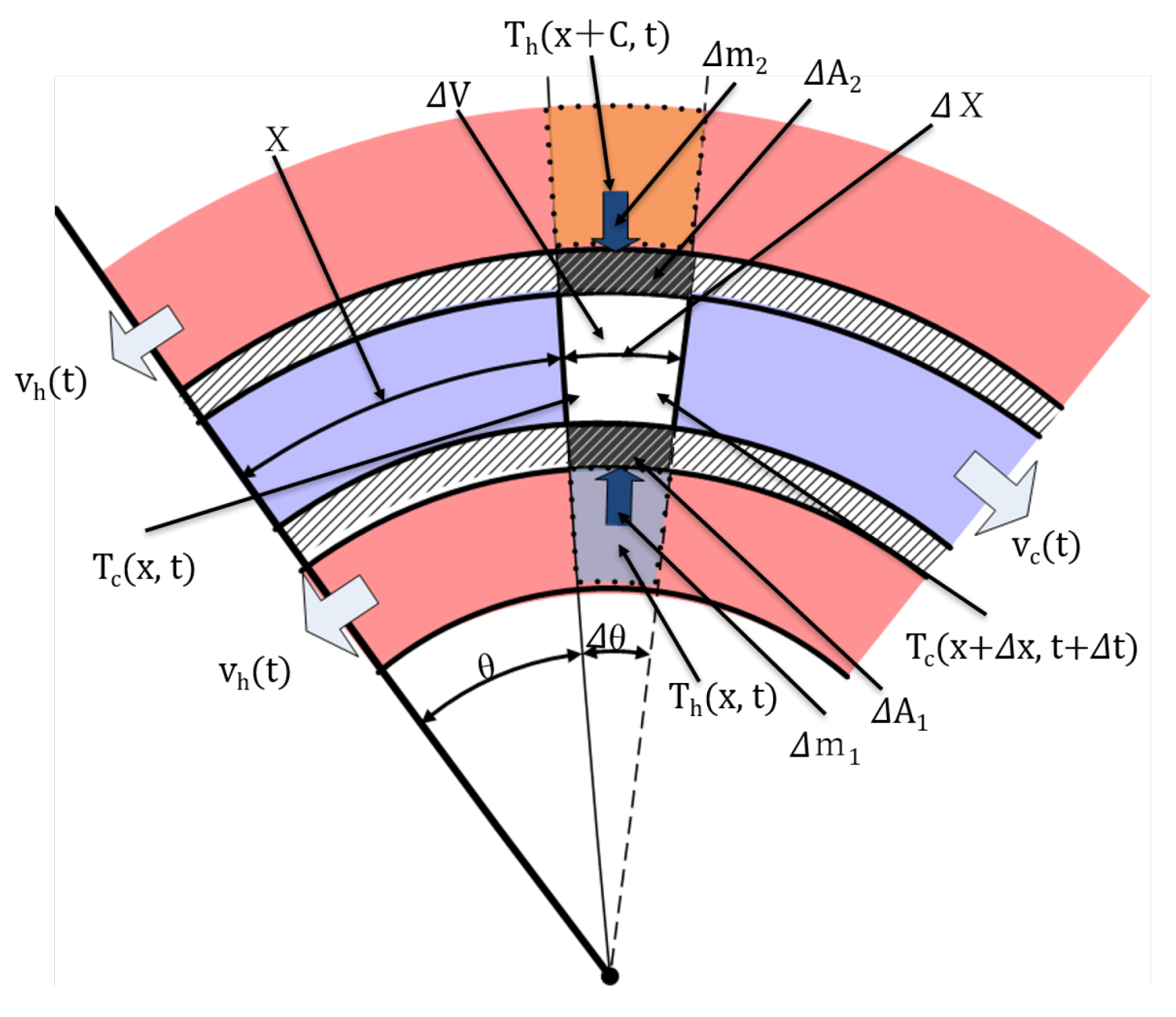
3.2. Fractional Order Derivative Model for the Spiral-Plate Counter-Flow Heat Exchanger
3.3. Fractional Order Derivative Model for the Spiral-Plate Parallel-Flow Heat Exchanger
4. Parallel Fractional Order Derivative Model for the Spiral-Plate Heat Exchanger and Implementation on GPU
4.1. Parallel Fractional Order Derivative Model for the Spiral-Plate Heat Exchanger
4.1.1. Parallel Model for the Spiral-Plate Counter-Flow Heat Exchanger
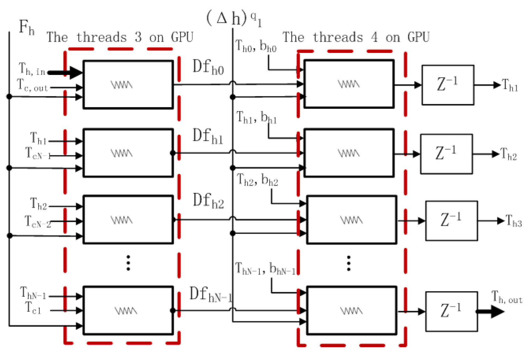
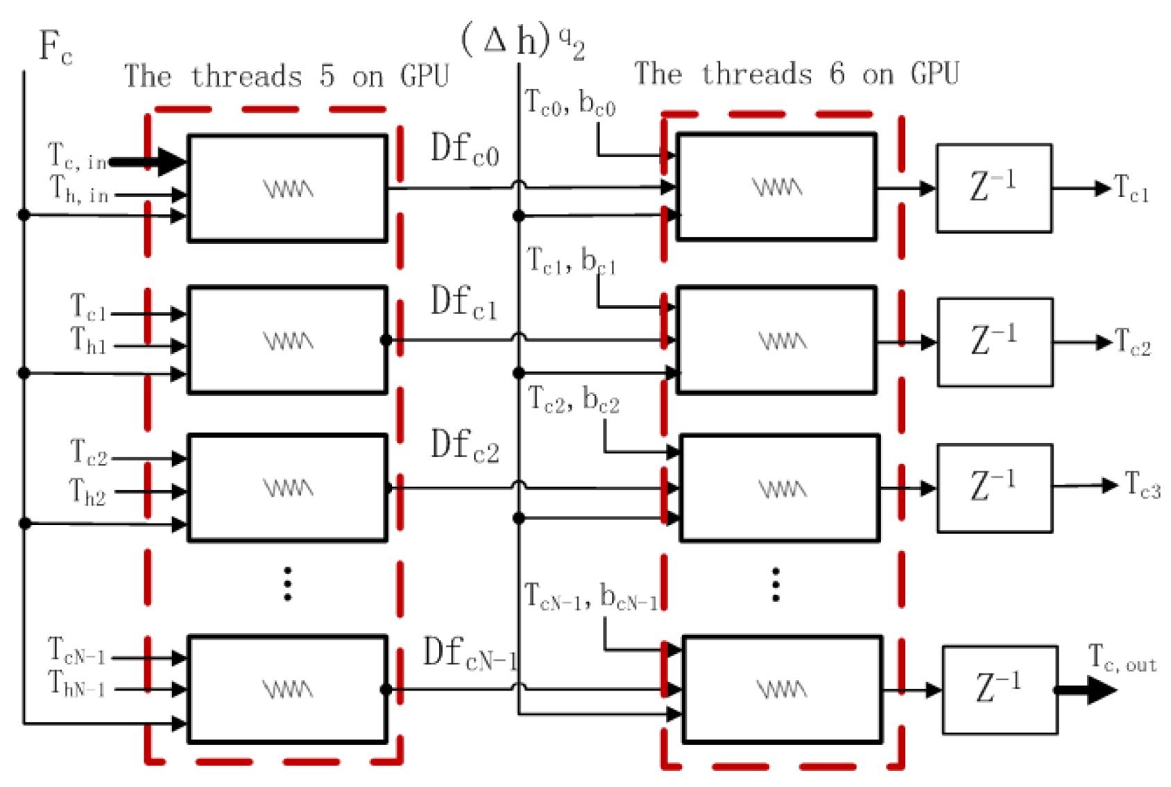
4.1.2. The Proposed Parallel Model for the Spiral-Plate Parallel-Flow Heat Exchanger
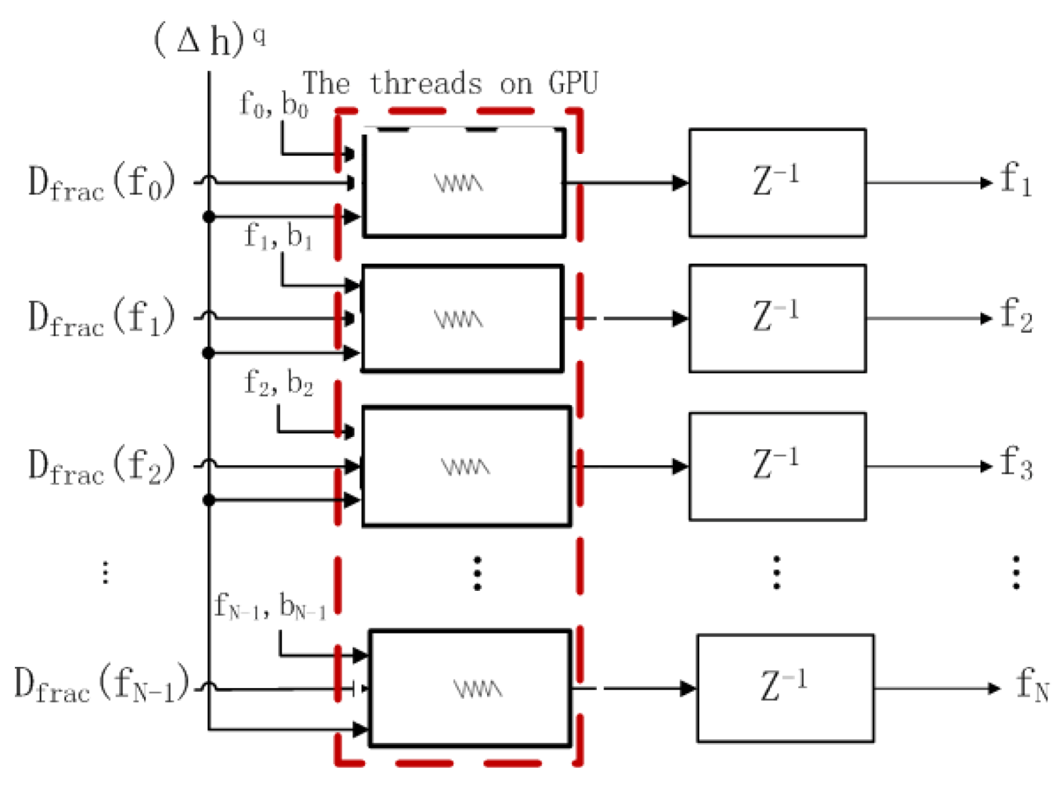
4.2. Implementation on GPU for the Proposed Parallel Model
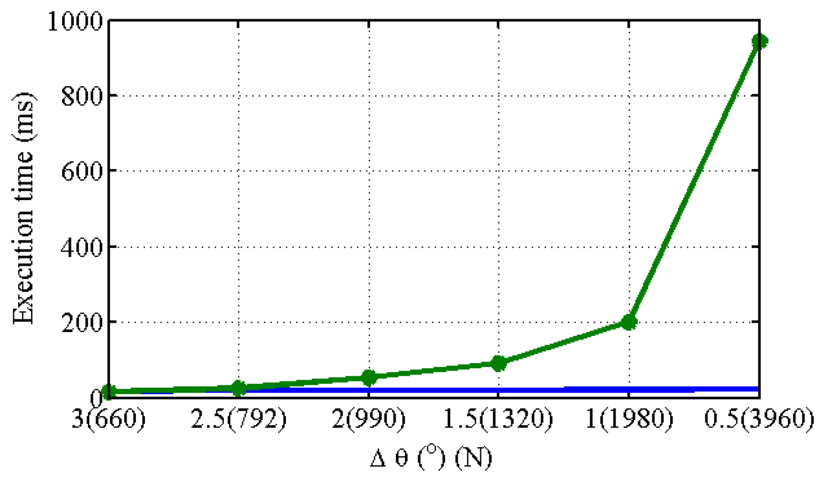
4.3. The Comparison of Execution Time for the Proposed Parallel Model on CPU and GPU
5. Simulation on the Proposed Parallel Model for the Spiral-Plate Heat Exchanger
5.1. Simulation Conditions
5.2. Simulation on the Proposed Parallel Model for the Spiral-Plate Counter-Flow Heat Exchanger
5.2.1. Simulation with the Different Fractional Orders as
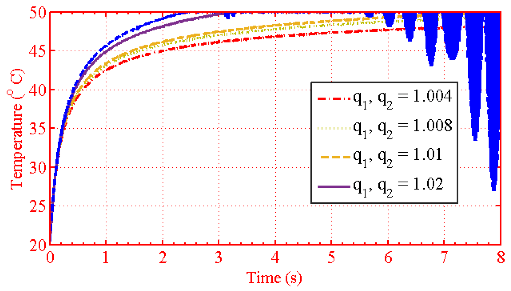
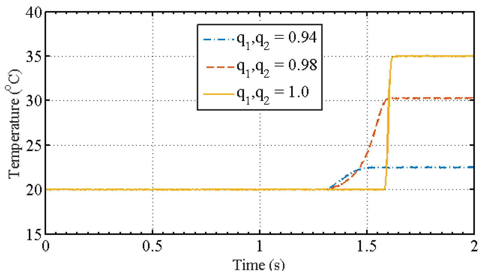
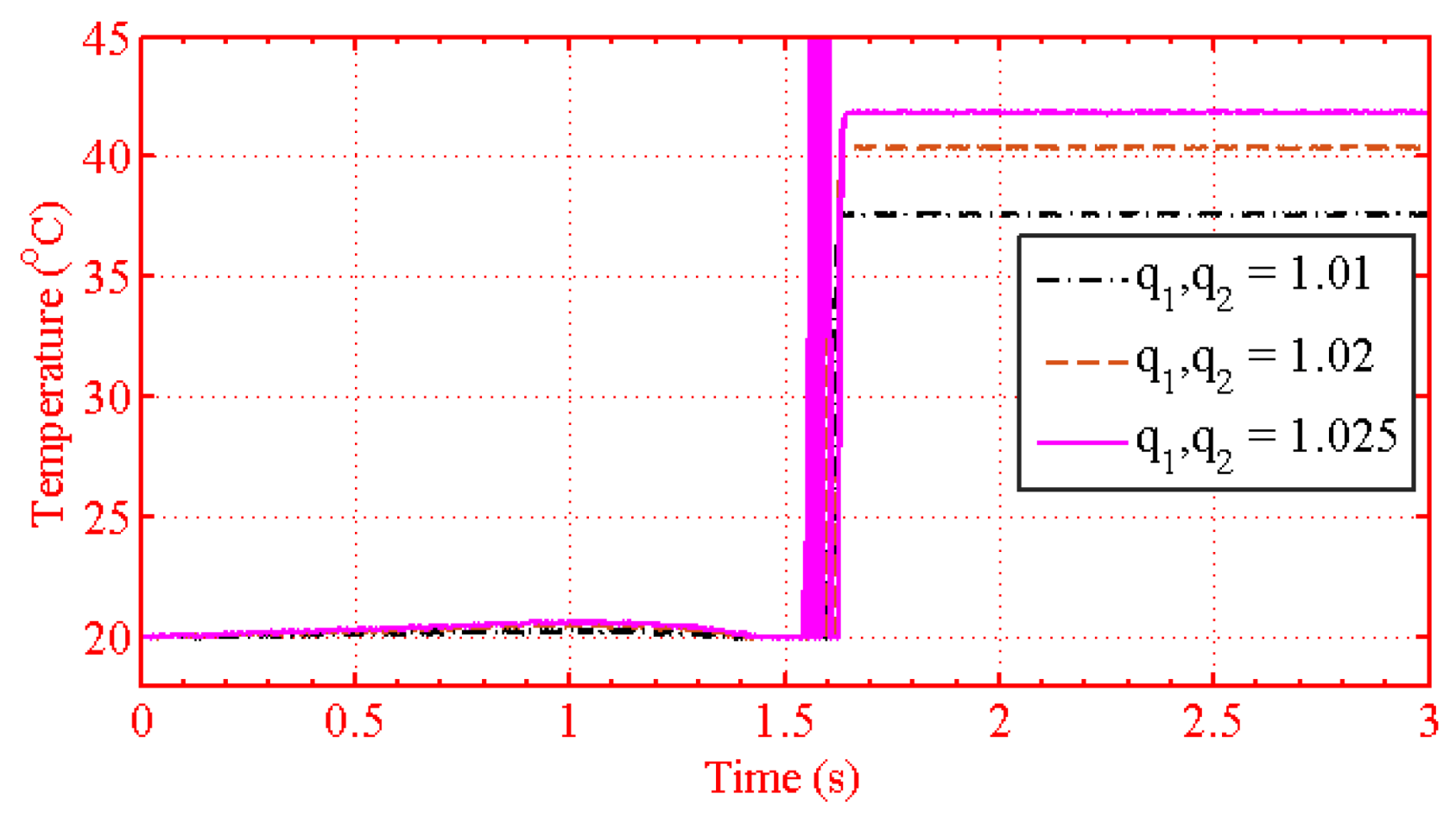
5.2.2. Simulation with the Different Fractional Orders as ,
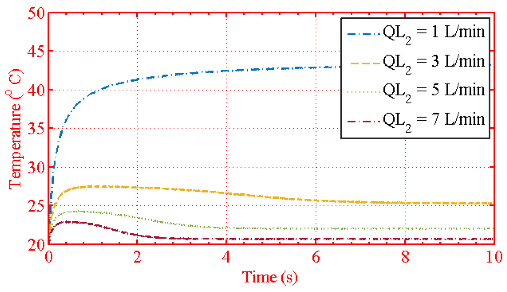
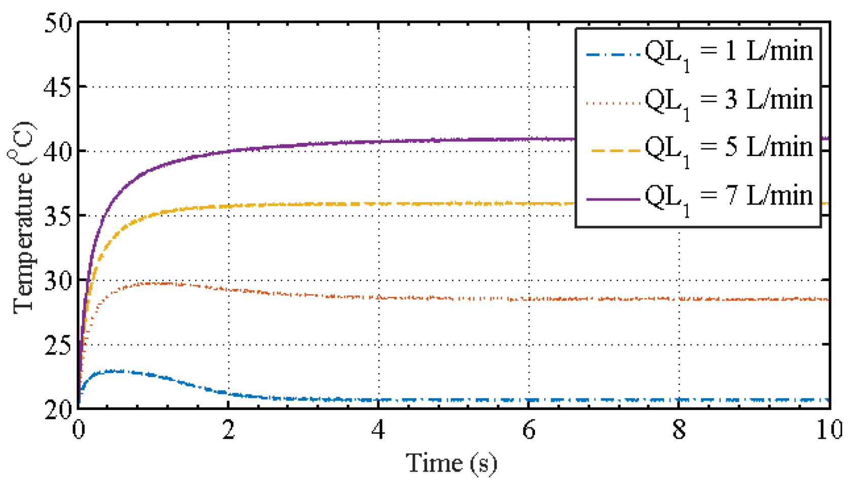
5.2.3. The Relationships between the Output Temperature in Cold Fluid and the Different Volume Flow Rate of Hot Fluid
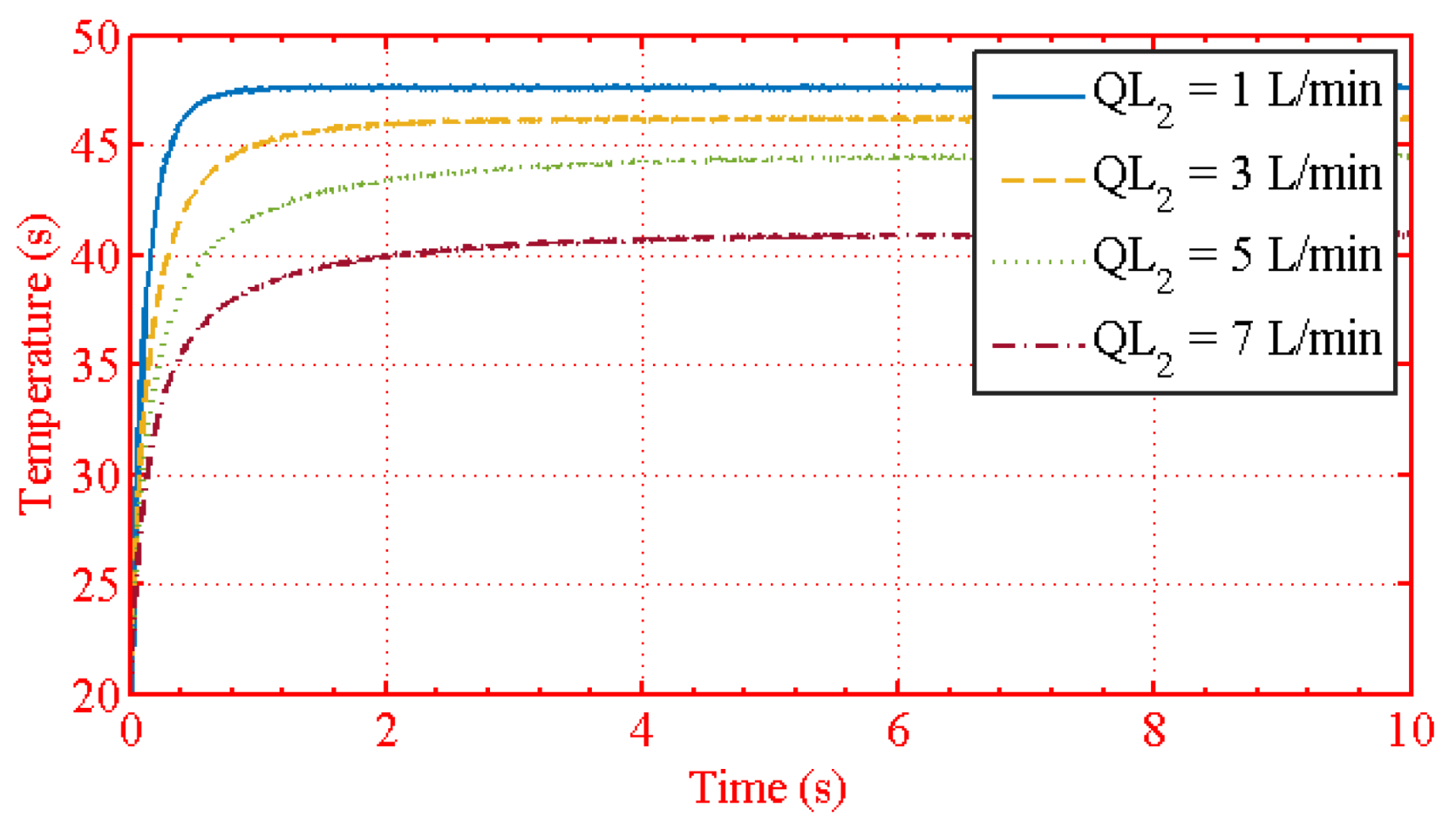
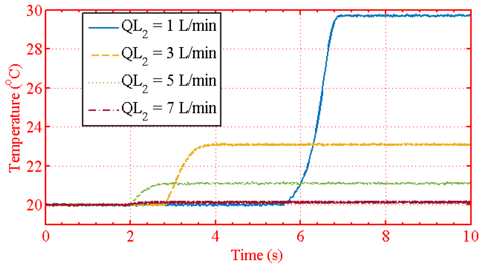
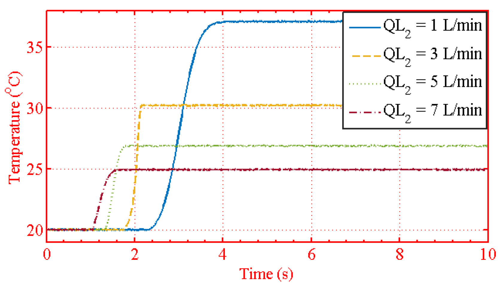
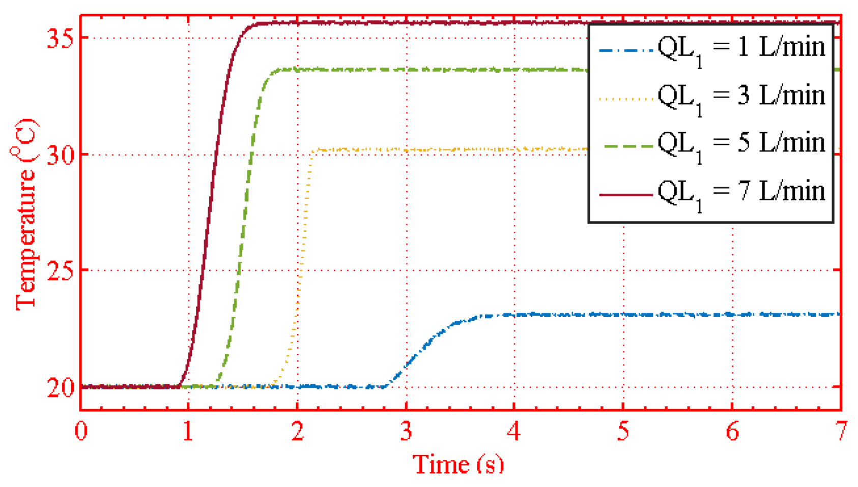
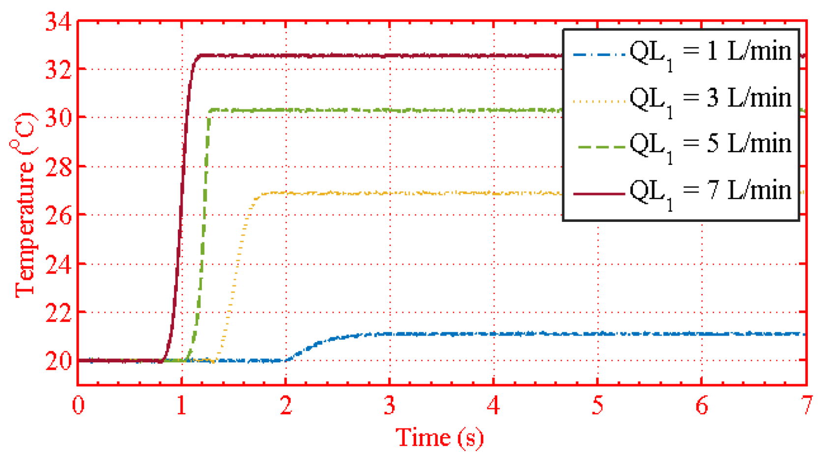
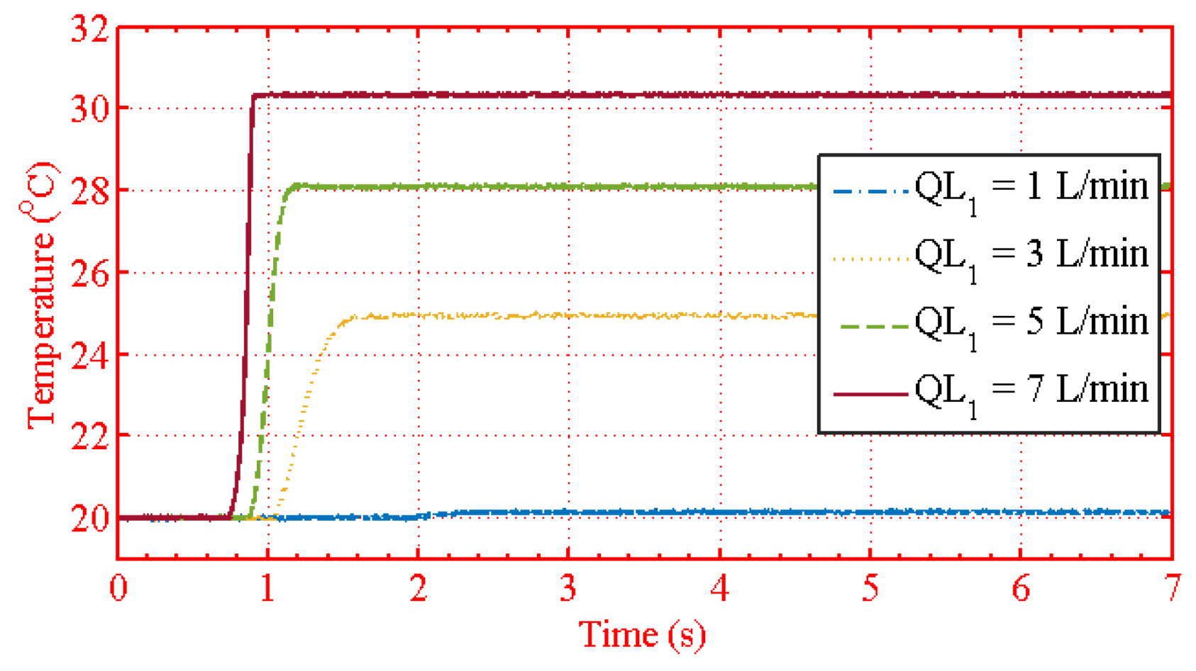
5.2.4. The Relationships between the Output Temperature in Cold Fluid and the Different Volume Flow Rate of Cold Fluid
5.3. Simulation on the Proposed Parallel Model for the Spiral-Plate Parallel-Flow Heat Exchanger
5.3.1. Simulation with the Different Fractional Orders as
5.3.2. Simulation with the Different Fractional Orders as ,
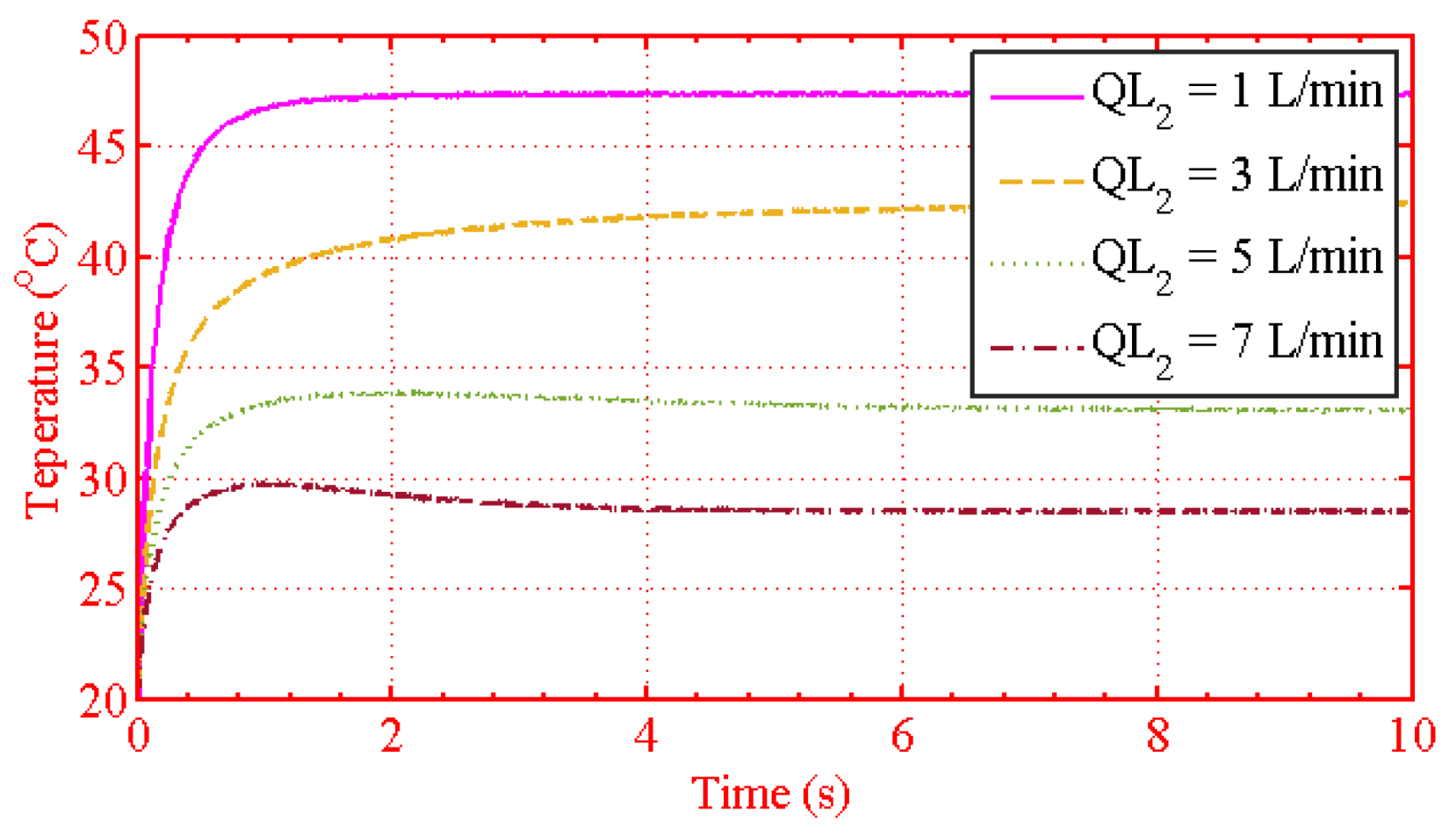
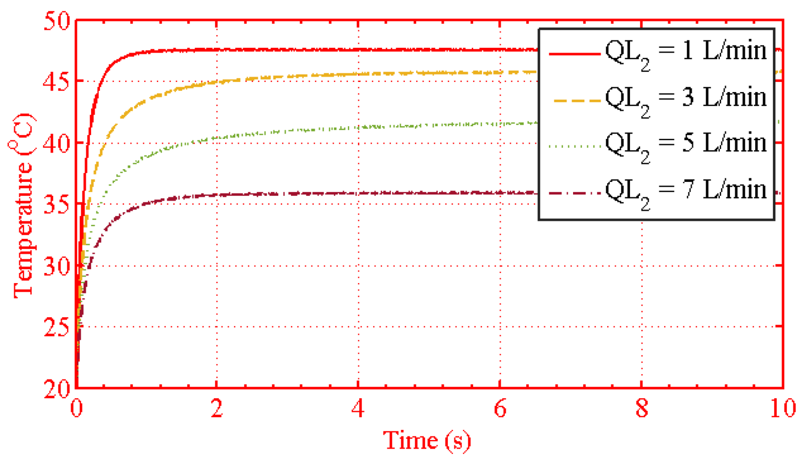
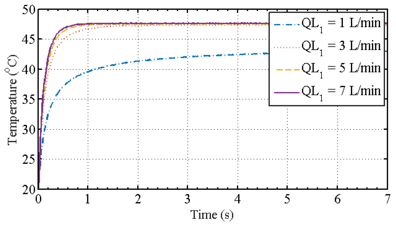
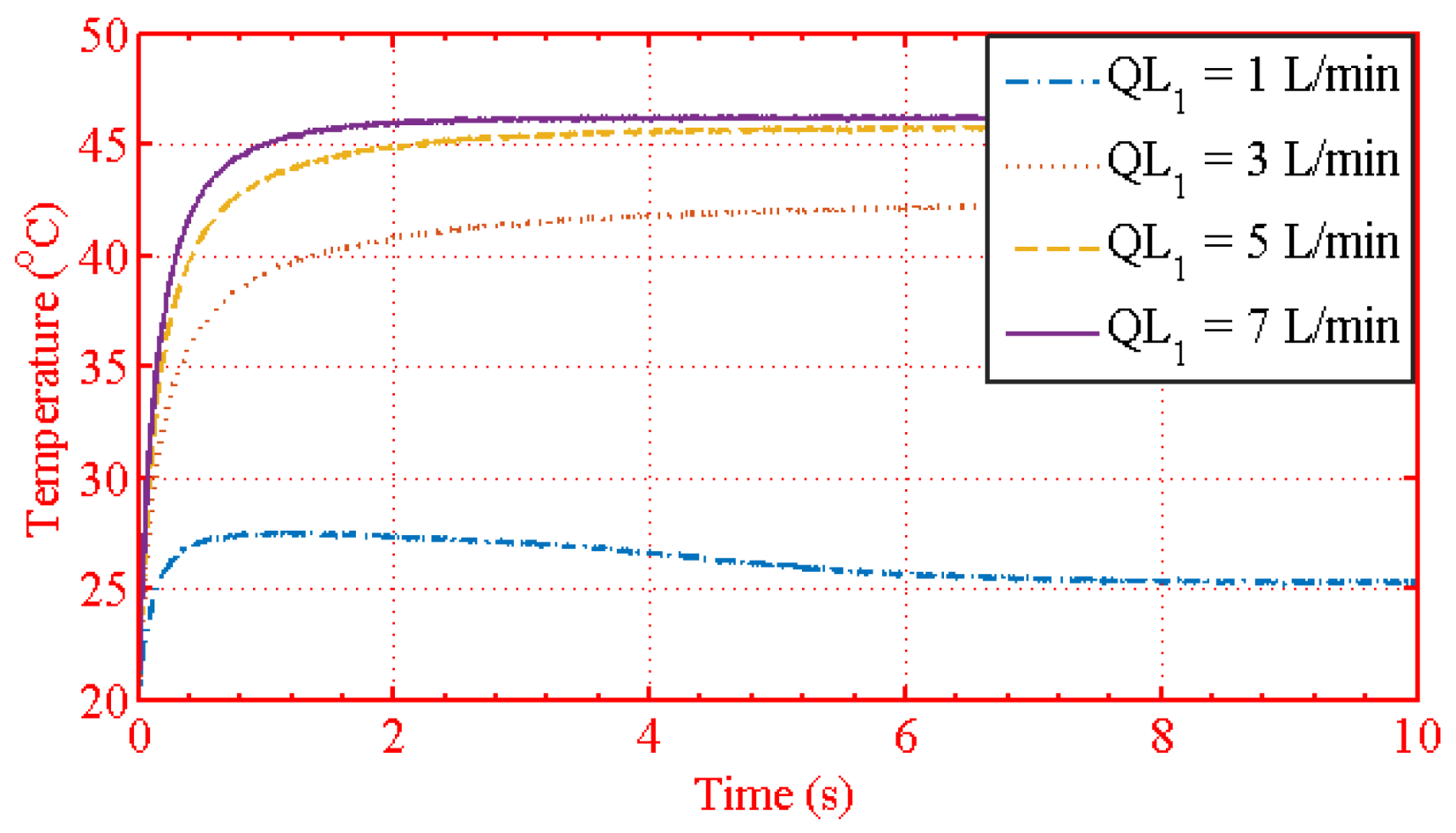
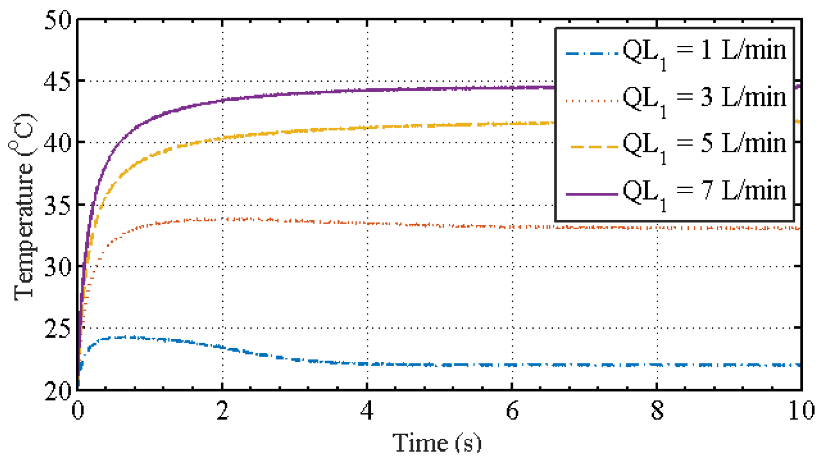
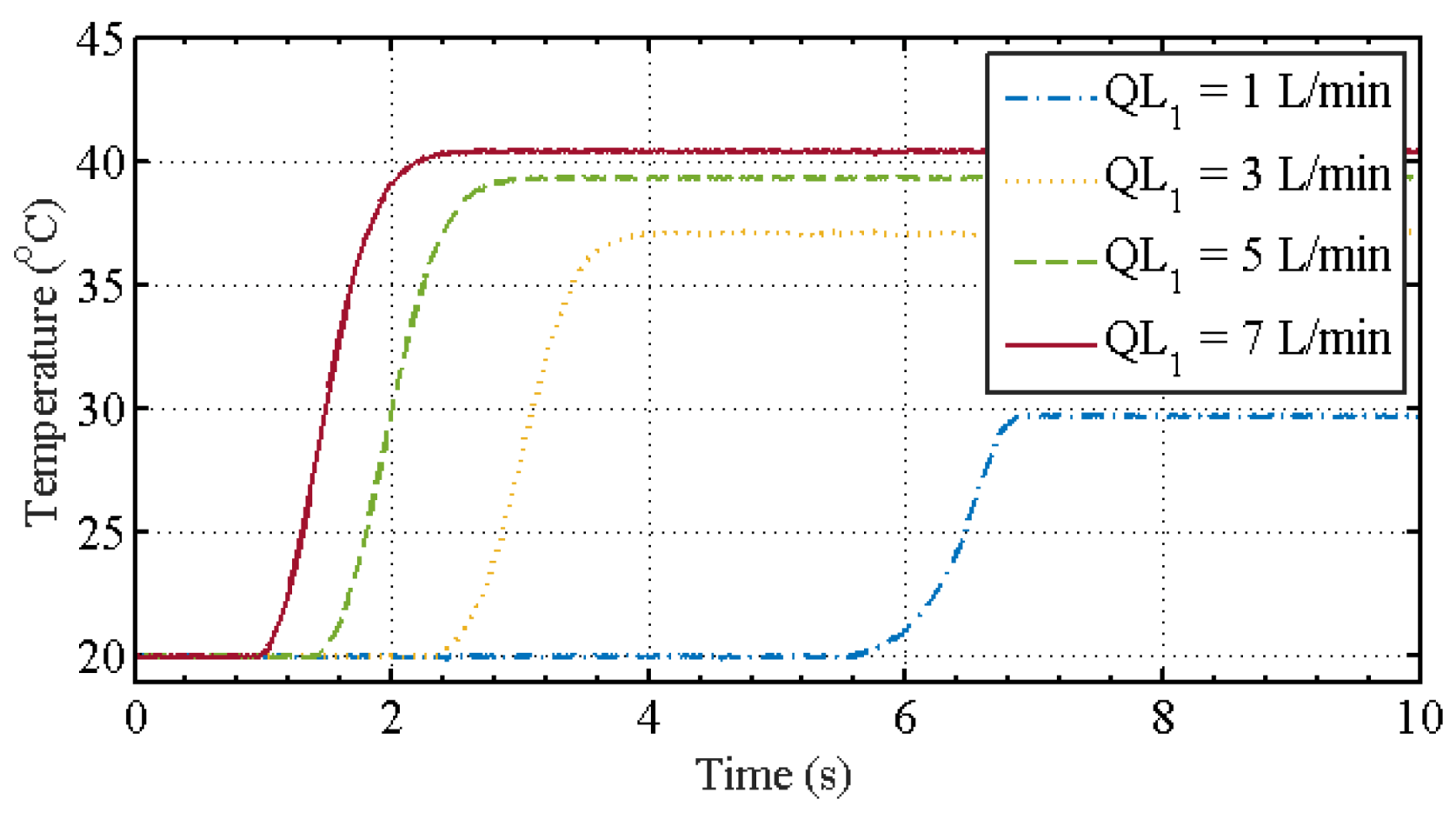
5.3.3. The Relationships between the Output Temperature of Cold Fluid and the Different Volume Flow Rate of Hot Fluid
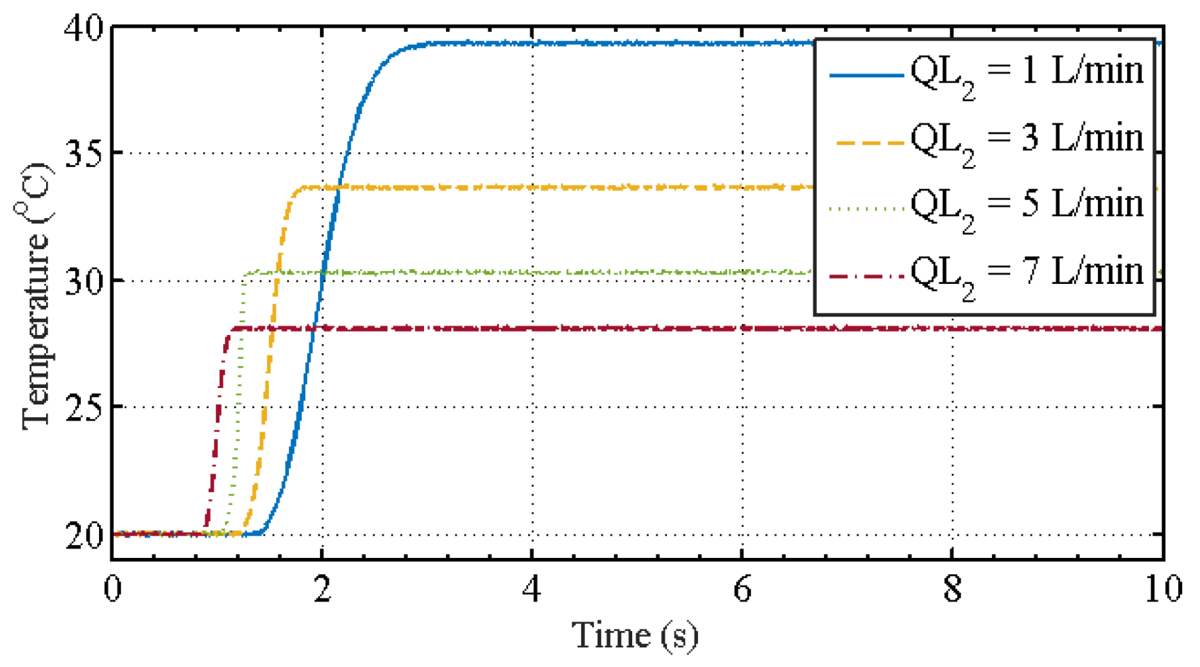
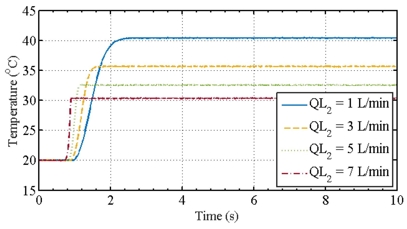
5.3.4. The Relationships between the Output Temperature of Cold Fluid and the Different Volume Flow Rate of Cold Fluid
6. Conclusions
Author Contributions
Funding
Institutional Review Board Statement
Informed Consent Statement
Data Availability Statement
Conflicts of Interest
Appendix A
References
- Tapre, R.W.; Kaware, J.P. Review on heat transfer in spiral heat exchanger. Int. J. Sci. Res. 2015, 5, 1–5. [Google Scholar]
- Sathiyan, S.; Rangarajan, M. An experimental study of spiral-plate heat exchanger for nitrobenzene-water two-phase system. Bulg. Chem. Commun. 2010, 42, 205–209. [Google Scholar]
- Khorshidi, J.; Heidari, S. Design and construction of a spiral heat exchanger. Adv. Chem. Eng. Sci. 2016, 6, 201–298. [Google Scholar] [CrossRef]
- Memon, S.; Gadhe, P.; Kulkarni, S. Design and testing of a spiral plate heat exchanger for textile industry. Int. J. Sci. Eng. Res. 2019, 10, 149–157. [Google Scholar]
- Metta, V.R.; Konijeti, R.; Dasore, A. Thermal design of spiral plate heat exchanger through numerical modelling. Int. J. Mech. Eng. Technol. 2018, 9, 736–745. [Google Scholar]
- Gomadam, P.M.; White, R.E.; Weidner, J.W. Modeling heat conduction in spiral geometries. J. Electrochem. Soc. 2003, 150, A1339–A1345. [Google Scholar] [CrossRef]
- Bidabadi, M.; Sadaghiani, A.K.; Azad, A.V. Spiral heat exchanger optimization using genetic algorithm. Sci. Iran. B 2013, 20, 1445–1454. [Google Scholar]
- Wen, S.; Deng, M. Operator-based robust nonlinear control and fault detection for a Peltier actuated thermal process. Math. Comput. Model. 2012, 57, 16–29. [Google Scholar] [CrossRef]
- Fujii, R.; Deng, M.; Wakitani, S. Nonlinear remote temperature control of a spiral plate heat exchanger. In Proceedings of the 2015 International Conference on Advanced Mechatronic Systems, Beijing, China, 22–24 August 2015; pp. 533–537. [Google Scholar]
- Podlubny, I. Fractional Differential Equations; Academic Press: Cambridge, MA, USA, 1999. [Google Scholar]
- Jafari, H.; Khalique, C.M.; Nazari, M. An algorithm for the numerical solution of nonlinear fractional-order Van der Pol oscillator equation. Math. Comput. Model. 2012, 55, 1782–1786. [Google Scholar] [CrossRef]
- Ibrahim, R.W.; Darus, M. On a new solution of factional differential equation using complex transform in the unit disk. Math. Comput. Appl. 2014, 19, 152–160. [Google Scholar]
- Qian, D.; Li, C.; Agarwal, R.P. Stability analysis of fractional differential system with Riemann–Liouville derivative. Math. Comput. Model. 2010, 52, 862–874. [Google Scholar]
- Baranowski, J.; Zagorowska, M.; Bauer, W.; Dziwinski, T.; Piatek, P. Applications of Direct Lyapunov Method in Caputo Non-Integer Order Systems. Elektron. Elektrotechnika 2015, 21, 10–13. [Google Scholar] [CrossRef][Green Version]
- Li, Y.; Chen, Y.; Podlubny, I. Mittag–Leffler stability of fractional order nonlinear dynamic systems. Automatica 2009, 45, 1965–1969. [Google Scholar] [CrossRef]
- Caponetto, R.; Dongola, G.; Fortuna, L.; Petras, I. Fractional Order Systems: Modeling and Control Applications; World Scientific: Singapore, 2010. [Google Scholar]
- Patnaik, S.; Sidhardh, S.; Semperlotti, F. Nonlinear thermoelastic fractional-order model of nonlocal plates: Application to postbuckling and bending response. Thin-Walled Struct. 2021, 164, 107809. [Google Scholar] [CrossRef]
- Challamel, N.; Zorica, D.; Atanacković, T.M.; Spasić, D.T. On the fractional generalization of Eringen’s nonlocal elasticity for wave propagation. Comptes Rendus Mécanique 2013, 341, 298–303. [Google Scholar] [CrossRef]
- Sidhardh, S.; Patnaik, S.; Semperlotti, F. Thermodynamics of fractional-order nonlocal continua and its application to the thermoelastic response of beams. Eur. J. Mech. A/Solids 2021, 88, 104238. [Google Scholar] [CrossRef]
- Monje, C.A.; Chen, Y.; Vinagre, B.M.; Xue, D.; Feliu, V. Fractional Order Systems and Controls: Fundamentals and Applications; Springer: Berlin/Heidelberg, Germany, 2010. [Google Scholar]
- Oldham, K.B.; Spanier, J. The Fractional Calculus: Theory and Applications of Differentiation and Integration to Arbitrary Order; Dover Publications: Mineola, NY, USA, 2006. [Google Scholar]
- Magin, R.L.; Ovadia, M. Modeling the cardiac tissue electrode interface using fractional calculus. J. Vib. Control 2008, 14, 1431–1442. [Google Scholar] [CrossRef]
- Padovan, J. Computational algorithms for FE formulations involving fractional operator. Comput. Mech. 1987, 2, 271–287. [Google Scholar] [CrossRef]
- Zhong, L. Comparative analysis of GPU and CPU. Technol. Mark. 2009, 9, 13–14. [Google Scholar]
- Liu, S.; Liu, M.; Zhang, G. Model of accelerating MATLAB computation based on CUDA. Appl. Res. Comput. 2010, 6, 2140–2143. [Google Scholar]
- Povstenko, Y. Fractional Thermoelasticity; Springer International Publishing: Berlin/Heidelberg, Germany, 2015. [Google Scholar]
- Challamel, N.; Grazide, C.; Picandet, V.; Perrot, A.; Zhang, Y. A nonlocal Fourier’s law and its application to the heat conduction of one-dimensional and two-dimensional thermal. Comptes Rendus Mécanique 2016, 344, 388–401. [Google Scholar] [CrossRef]
- Sumelka, W. Thermoelasticity in the Framework of the Fractional Continuum Mechanics. J. Therm. Stress. 2014, 37, 678–706. [Google Scholar] [CrossRef]
- Deng, M.; Wen, S.; Inoue, A. Operator-based robust nonlinear control for a Peltier actuated process. Meas. Control. J. Inst. Meas. Control. 2011, 44, 116–120. [Google Scholar] [CrossRef]
- Bi, S.; Deng, M.; Xiao, Y. Robust Stability and Tracking for Operator-Based Nonlinear Uncertain Systems. IEEE Trans. Autom. Sci. Eng. 2015, 12, 1059–1066. [Google Scholar] [CrossRef]
- Deng, M.; Kawashima, T. Adaptive Nonlinear Sensorless Control for an Uncertain Miniature Pneumatic Curling Rubber Actuator Using Passivity and Robust Right Coprime Factorization. IEEE Trans. Control Syst. Technol. 2016, 24, 318–324. [Google Scholar] [CrossRef]
- Dong, G.; Deng, M. Modeling of a spiral heat exchanger using fractional order equation and GPU. In Proceedings of the 2019 International Conference on Advanced Mechatronic Systems (ICAMechS), Kusatsu, Japan, 26–28 August 2019; pp. 108–113. [Google Scholar]
- Magadum, A.; Pawar, A.; Patil, R.; Phadtare, R.; Mestri, T.C. Review of experimental analysis of parallel and counter flow heat exchanger. Int. J. Eng. Res. Technol. 2016, 5, 395–397. [Google Scholar]
- Bergman, T.; Lavine, A.; Incropera, F.; Dewitt, D. Faundamentals of Heat and Mass Transfer, 8th ed.; Wiley: Hoboken, NJ, USA, 2017. [Google Scholar]


| Meaning | Symbol | Value |
|---|---|---|
| Geometric parameter of a spiral function | a | 0.005/ m/rad |
| Initial radius of hot fluid side | b | 0.08 m |
| The width of hot flow channel | 0.005 m | |
| The width of cold flow channel | 0.005 m | |
| The width of solid wall | 0.0018 m | |
| The height of the spiral-plate heat exchanger | Z | 0.011 m |
| Figure No. | Description |
|---|---|
| Figure 4 | The thread block of the proposed parallel model |
| Figure 5 | That of cold fluid for the counter-flow heat exchanger |
| Figure 6 | That of hot fluid side for the counter-flow heat exchanger |
| Figure 7 | That of cold fluid side for the parallel-flow heat exchanger |
| Figure 8 | That of hot fluid side for the parallel-flow heat exchanger |
| Meaning | Symbol | Value |
|---|---|---|
| The densities of the two fluids | , | 1000 Kg/m |
| The specific heat capacity of the two fluids | , | 4.2 KJ/(Kg · °C) |
| The input temperature of cold fluid | 20 °C | |
| The input temperature of hot fluid | 50 °C | |
| Thermal conductivity of SUS304 | 16.7 W/(m °C) | |
| Heat transfer coefficients of the two fluids | , | 366 w/m · K |
| The orders for fractional order derivative | , | 0.9–1.02 |
| The volume flow rate of hot fluid | 1–7 L/min | |
| The volume flow rate of cold fluid | 1–7 L/min | |
| Correction factor | F | 1.8 |
| Simulation time | t | [0, 12] s |
| Figure No. | Descrption |
|---|---|
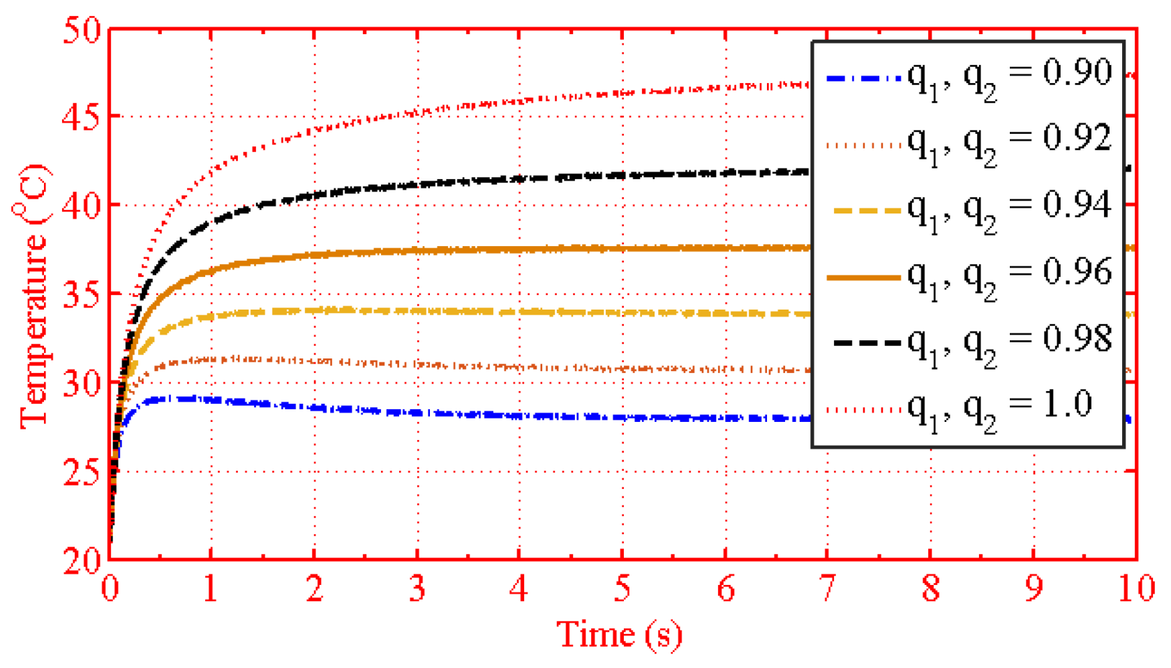
| Figure 10 | , = 0.9, 0.92, 0.94, 0.96, 0.98, 1.0 |
| Figure 11 | , = 1.004, 1.008, 1.01, 1.02 |
| Figure 12 | = 1 L/min, = 1, 3, 5, 7 L/min |
| Figure 13 | = 3 L/min, = 1, 3, 5, 7 L/min |
| Figure 14 | = 5 L/min, = 1, 3, 5, 7 L/min |
| Figure 15 | = 7 L/min, = 1, 3, 5, 7 L/min |
| Figure 16 | = 1, 3, 5, 7 L/min, = 1 L/min |
| Figure 17 | = 1, 3, 5, 7 L/min, = 3 L/min |
| Figure 18 | = 1, 3, 5, 7 L/min, = 5 L/min |
| Figure 19 | = 1, 3, 5, 7 L/min, = 7 L/min |
| Figure No. | Descrption |
|---|---|
| Figure 20 | , = 0.9, 0.92, 0.94, 0.96, 0.98, 1.0 |
| Figure 21 | , = 1.004, 1.008, 1.01, 1.02 |
| Figure 22 | =1 L/min, = 1, 3, 5, 7 L/min |
| Figure 23 | =3 L/min, = 1, 3, 5, 7 L/min |
| Figure 24 | =5 L/min, = 1, 3, 5, 7 L/min |
| Figure 25 | =7 L/min, = 1, 3, 5, 7 L/min |
| Figure 26 | = 1, 3, 5, 7 L/min, = 1 L/min |
| Figure 27 | = 1, 3, 5, 7 L/min, = 3 L/min |
| Figure 28 | = 1, 3, 5, 7 L/min, = 5 L/min |
| Figure 29 | = 1, 3, 5, 7 L/min, = 7 L/min |
Publisher’s Note: MDPI stays neutral with regard to jurisdictional claims in published maps and institutional affiliations. |
© 2021 by the authors. Licensee MDPI, Basel, Switzerland. This article is an open access article distributed under the terms and conditions of the Creative Commons Attribution (CC BY) license (https://creativecommons.org/licenses/by/4.0/).
Share and Cite
Dong, G.; Deng, M. GPU Based Modelling and Analysis for Parallel Fractional Order Derivative Model of the Spiral-Plate Heat Exchanger. Axioms 2021, 10, 344. https://doi.org/10.3390/axioms10040344
Dong G, Deng M. GPU Based Modelling and Analysis for Parallel Fractional Order Derivative Model of the Spiral-Plate Heat Exchanger. Axioms. 2021; 10(4):344. https://doi.org/10.3390/axioms10040344
Chicago/Turabian StyleDong, Guanqiang, and Mingcong Deng. 2021. "GPU Based Modelling and Analysis for Parallel Fractional Order Derivative Model of the Spiral-Plate Heat Exchanger" Axioms 10, no. 4: 344. https://doi.org/10.3390/axioms10040344
APA StyleDong, G., & Deng, M. (2021). GPU Based Modelling and Analysis for Parallel Fractional Order Derivative Model of the Spiral-Plate Heat Exchanger. Axioms, 10(4), 344. https://doi.org/10.3390/axioms10040344