Abstract
This paper establishes a model of economic growth for all the G7 countries from 1973 to 2016, in which the gross domestic product (GDP) is related to land area, arable land, population, school attendance, gross capital formation, exports of goods and services, general government, final consumer spending and broad money. The fractional-order gradient descent and integer-order gradient descent are used to estimate the model parameters to fit the GDP and forecast GDP from 2017 to 2019. The results show that the convergence rate of the fractional-order gradient descent is faster and has a better fitting accuracy and prediction effect.
MSC:
26A33
1. Introduction
In recent years, fractional model has become a research hotspot because of its advantages. Fractional calculus has developed rapidly in academic circles, and its achievements in the fields include [1,2,3,4,5,6,7,8,9,10].
Gradient descent is generally used as a method of solving the unconstrained optimization problems, and is widely used in evaluation and in other aspects. The rise in fractional calculus provides a new idea for advances in the gradient descent method. Although numerous achievements have been made in the two fields of fractional calculus and gradient descent, the research results combining the two are still in their infancy. Recently, ref. [11] applied the fractional order gradient descent to image processing and solved the problem of blurring image edges and texture details using a traditional denoising method, based on integer order. Next, ref. [12] improved the fractional-order gradient descent method and used it to identify the parameters of the discrete deterministic system in advance. Thereafter, ref. [13] applied the fractional-order gradient descent to the training of neural networks’ backpropagation (BP), which proves the monotony and convergence of the method.
Compared with the traditional integer-order gradient descent, the combination of fractional calculus and gradient descent provides more freedom of order; adjusting the order can provide new possibilities for the algorithm. In this paper, economic growth models of seven countries are established, and their cost functions are trained by gradient descent (fractional- and integer-order). To compare the performance of fractional- and integer-order gradient descent, we visualize the rate of convergence of the cost function, evaluate the model with , and indicators and predict the GDP of the seven countries in 2017–2019 according to the trained parameters.
The Group of Seven (G7)
The G6 was set up by France after western countries were hit by the first oil shock. In 1976, Canada’s accession marked the birth of the G7, whose members are the United States, the United Kingdom, France, Germany, Japan, Italy and Canada seven developed countries. The annual summit mechanism of the G7 focuses on major issues of common interest, such as inclusive economic growth, world peace and security, climate change and oceans, which have had a profound impact on global, economic and political governance. In addition to the G7 members, there are a number of developing countries with large economies, such as China, India and Brazil. In the context of economic globalization, the study of G7 economic trends and economic-related factors can provide a useful reference for these countries’ development.
The economic crisis broke out in western countries in 1973, so the data in this paper cover the period from 1973 to 2016, and data for the seven countries are available since then. Some G7 members (France, Germany, Italy and the United States) were members of the European Union (EU) during this period, so this paper also establishes the economic growth model of the EU. Data for this article are from the World Bank.
2. Model Describes
The prediction of variables generally uses time series models [14] (for example, ARIMA and SARIMA), or artificial neural networks [15,16], which have been very popular in recent years. The time series model mainly predicts the future trend in variables, but it is difficult to reflect the change in unexpected factors in the model. Additionally, the neural network model needs to adjust more parameters, the network structure selection is too large, the training efficiency is not high enough, and easy to overfit.
Although the linear model is simple in form and easy to model, its weight can intuitively express the importance of each attribute, so the linear model has a good explanatory ability. It is reasonable to build a linear regression model of economic growth, which can clearly learn which factors have an impact on the economy.
Next, we chose eight explanatory variables to describe the economic growth in this paper. The explained variable is y, where y refers to GDP and is a function. The expression for y is as follows:
where t is year (), is the intercept. is an unobservable term of random error. represents the weight of each variable. The eight explanatory variables are:
- : land area (km)
- : arable land (hm)
- : population
- : school attendance (years)
- : gross capital formation (in 2010 US$)
- : exports of goods and services (in 2010 US$)
- : general government final consumer spending (in 2010 US$)
- : broad money (in 2010 US$)
3. Fractional-Order Derivative
Due to the differing conditions, there are different forms of fractional calculus definition, the most common of which are Grnwald–Letnikov, Riemann–Liouville, and Caputo. In this article, we chose the definition of fractional-order derivative in terms of the Caputo form. Given the function , the Caputo fractional-order derivative of order is defined as follows:
where is the Caputo derivative operator. is the fractional order, and the interval is . is the gamma function. c is the initial value. For simplicity, is used in this paper to represent the Caputo fractional derivative operator instead .
Caputo fractional differential has good properties. For example, we provide the Laplace transform of Caputo operator as follows:
where is a generalized integral with a complex parameter s, . is the rounded up to the nearest integer. It can be seen from the Laplace transform that the definition of the initial value of Caputo differentiation is consistent with that of integer-order differential equations and has a definite physical meaning. Therefore, Caputo fractional differentiation has a wide range of applications.
4. Gradient Descent Method
4.1. The Cost Function
The cost function (also known as the loss function) is essential for a majority of algorithms in machine learning. The model’s optimization is the process of training the cost function, and the partial derivative of the cost function with respect to each parameter is the gradient mentioned in gradient descent. To select the appropriate parameters for the model (1) and minimize the modeling error, we introduce the cost function:
where is a modification of model (1), , which represents the output value of the model. are the sample features. is the true data, and t represents the number of samples ().
4.2. The Integer-Order Gradient Descent
The first step of the integer-order gradient descent is to take the partial derivative of the cost function :
and the update function is as follows:
where is learning rate, .
4.3. The Fractional-Order Gradient Descent
The first step of fractional-order gradient descent is to find the fractional derivative of the cost function . According to Caputo’s definition of fractional derivative, from [17] we know that if is a compound function of t, then the fractional derivation of with respect to t is
It can be known from (5) that the fractional derivative of a composite function can be expressed as the product of integral and fractional derivatives. Therefore, the calculation for is as follows:
and the update function is as follows:
where is the learning rate, . is the fractional order, . c is the initial value of Caputo’s fractional derivative, and .
5. Model Evaluation Indexes
We use the absolute relative error () to measure the prediction error:
To evaluate the fitting quality of gradient descent on the model, the following three indicators can be calculated:
The mean square error ():
The coefficient of determination ():
The mean absolute deviation ():
In these formulas, n is the number of years (). and are the real value and the model output, respectively. is the mean of the GDP.
6. Main Results
In this article, we standardize the data for each country before running the algorithm, and each iteration to update uses m samples. The grid search method was used to select the appropriate learning rate and initial weight interval, and the effects of different fractional orders are compared to select the best order (see Table 1).The learning rate and the initial weight interval are applicable to both fractional-order gradient descent and integer-order gradient descent.

Table 1.
Parameters for different countries.
6.1. Comparison of Convergence Rate of Fractional and Integer Order Gradient Descent
In order to facilitate visual comparison, (4) and (6) are iterated 50 times, respectively, as well as their convergence rates (see Figure 1).
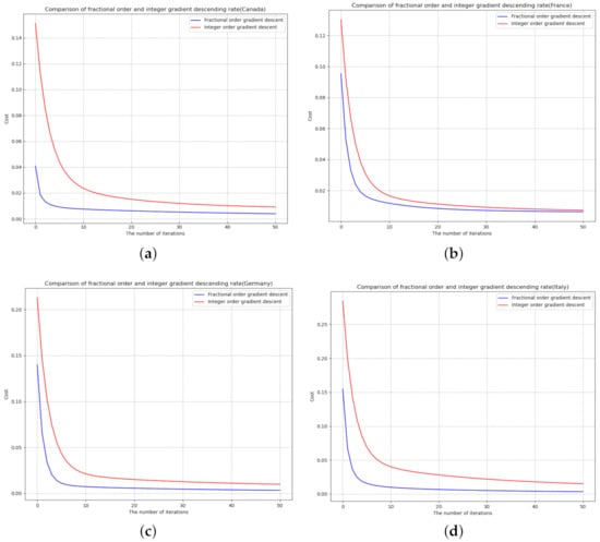
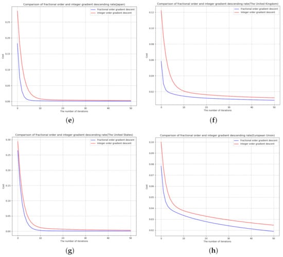
Figure 1.
Comparison of convergence rate and fitting error between fractional- and integer-order gradient descent: (a) Canada (b) France (c) Germany (d) Italy (e) Japan (f) The United Kingdom (g) The United States (h) European Union.
As shown in Figure 1, for each dataset, after the same number of iterations, the convergence rate of fractional-order gradient descent is faster than that of integer-order gradient descent, which indicates that the method combining fractional-order and gradient descent is better than the traditional integer-order gradient descent in the convergence rate of update equation.
6.2. Fitting Result
Then, we fit GDP with integer-order gradient descent and fractional-order gradient descent, respectively. Start by setting a threshold and stop iterating when the gradient is less than this threshold. The fitting effect diagram is shown in Figure 2, and the performance evaluation of the model is shown in Table 2.
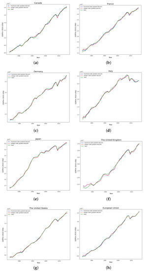
Figure 2.
Fitting of GDP of the G7 countries by fractional-order gradient descent method: (a) Canada (b) France (c) Germany (d) Italy (e) Japan (f) The United Kingdom (g) The United States (h) European Union.
Table 2.
Performance of integer order and fractional order gradient descent.
It can be seen from Table 2 that the , and results of GDP fitted by fractional-order gradient descent are better than that fitted by integer-order gradient descent, which indicates that, under the same iteration number, learning rate and initial weight interval, the fitting performance of the data fitted by fractional-order gradient descent is better than that of integer-order.
6.3. Predicted Results
Finally, in order to test the prediction effect of fractional- and integer-order gradient descent on GDP, we forecast the GDP from 2017 to 2019, and used the index to measure the prediction error (see Table 3).
Table 3.
Integer-order and fractional-order gradient descent for G7 countries’ GDP data from 2017 to 2019.
7. Conclusions
In this paper, the gradient descent method is used to study the linear model problems which is different from [18,19]. The results show that, in addition to the least square estimation, the gradient descent method can also solve the regression analysis problem by iterating the cost function, and obtain good results, a without complicating the model. It also improves the interpretability of explanatory variables. We apply the fractional differential to gradient descent, and compare the performance of fractional-order gradient descent with that of integer-order gradient descent. It was found that the fractional-order has a faster convergence rate, higher fitting accuracy and lower prediction error than the integer-order. This provides an alternative method for fitting and forecasting GDP and has a certain reference value.
Author Contributions
J.W. supervised and led the planning and execution of this research, proposed the research idea of combining fractional calculus with gradient descent, formed the overall research objective, and reviewed, evaluated and revised the manuscript. According to this research goal, X.W. collected data of economic indicators and applied statistics to create a model and used Python software to write codes to analyze data and optimize the model, and finally wrote the first draft. M.F. reviewed, evaluated and revised the manuscript. All authors have read and agreed to the published version of the manuscript.
Funding
This work is partially supported by Training Object of High Level and Innovative Talents of Guizhou Province ((2016)4006), Major Research Project of Innovative Group in Guizhou Education Department ([2018]012), the Slovak Research and Development Agency under the contract No. APVV-18-0308 and by the Slovak Grant Agency VEGA No. 1/0358/20 and No. 2/0127/20.
Institutional Review Board Statement
Not applicable.
Informed Consent Statement
Not applicable.
Data Availability Statement
Acknowledgments
The authors are grateful to the referees for their careful reading of the manuscript and valuable comments. The authors thank the help from the editor too.
Conflicts of Interest
The authors declare no conflict of interest.
References
- Wang, J.; Ahmed, G.; O’Regan, D. Topological structure of the solution set for fractional non-instantaneous impulsive evolution inclusions. J. Fixed Point Theory Appl. 2018, 20, 1–25. [Google Scholar] [CrossRef]
- Li, M.; Wang, J. Representation of solution of a Riemann-Liouville fractional differential equation with pure delay. Appl. Math. Lett. 2018, 85, 118–124. [Google Scholar] [CrossRef]
- Yang, D.; Wang, J.; O’Regan, D. On the orbital Hausdorff dependence of differential equations with non-instantaneous impulses. C. R. Acad. Sci. Paris, Ser. I 2018, 356, 150–171. [Google Scholar] [CrossRef]
- You, Z.; Fečkan, M.; Wang, J. Relative controllability of fractional-order differential equations with delay. J. Comput Appl. Math. 2020, 378, 112939. [Google Scholar] [CrossRef]
- Wang, J.; Fečkan, M.; Zhou, Y. A Survey on impulsive fractional differential equations. Frac. Calc. Appl. Anal. 2016, 19, 806–831. [Google Scholar] [CrossRef]
- Victor, S.; Malti, R.; Garnier, H.; Outstaloup, A. Parameter and differentiation order estimation in fractional models. Automatica 2013, 49, 926–935. [Google Scholar] [CrossRef]
- Tang, Y.; Zhen, Y.; Fang, B. Nonlinear vibration analysis of a fractional dynamic model for the viscoelastic pipe conveying fluid. Appl. Math. Model. 2018, 56, 123–136. [Google Scholar] [CrossRef]
- Li, W.; Ning, J.; Zhao, G.; Du, B. Ship course keeping control based on fractional order sliding mode. J. Shanghai Marit. Univ. 2020, 41, 25–30. [Google Scholar]
- Yasin, F.; Ali, A.; Kiavash, F.; Rohollah, M.; Ami, R. A fractional-order model for chronic lymphocytic leukemia and immune system interactions. Math. Methods Appl. Sci. 2020, 44, 391–406. [Google Scholar]
- Chen, L.; Altaf, M.; Abdon, A.; Sunil, K. A new financial chaotic model in Atangana-Baleanu stochastic fractional differential equations. Alex. Eng. 2021, 60, 5193–5204. [Google Scholar]
- Pu, Y.; Zhang, N.; Zhang, Y.; Zhou, J. A texture image denoising approach based on fractional developmental mathematics. Pattern Anal. Appl. 2016, 19, 427–445. [Google Scholar] [CrossRef]
- Cui, R.; Wei, Y.; Chen, Y. An innovative parameter estimation for fractional-order systems in the presence of outliers. Nonlinear Dyn. 2017, 89, 453–463. [Google Scholar] [CrossRef]
- Wang, J.; Wen, Y.; Gou, Y.; Ye, Z.; Chen, H. Fractional-order gradient descent learning of BP neural networks with Caputo derivative. Neural Netw. 2017, 89, 19–30. [Google Scholar] [CrossRef] [PubMed]
- Guo, J.; Dong, B. International rice price forecast based on SARIMA model. Price Theory Pract. 2019, 1, 79–82. [Google Scholar]
- Xu, Y.; Chen, Y. Comparison between seasonal ARIMA model and LSTM neural network forecast. Stat. Decis. 2021, 2, 46–50. [Google Scholar]
- Wang, X.; Wang, J.; Fečkan, M. BP neural network calculus in economic growth modeling of the Group of Seven. Mathematics 2020, 8, 37. [Google Scholar] [CrossRef] [Green Version]
- Boroomand, A.; Menhaj, M. Fractional-order Hopfield neural networks. In Advances in Neuro-Information Processing, ICONIP 2008; Lecture Notes in Computer Science; Springer: Berlin/Heidelberg, Germany, 2009; Volume 5506, pp. 883–890. [Google Scholar]
- Tejado, I.; Pérez, E.; Valério, D. Fractional calculus in economics growth modeling of the Group of Seven. Fract. Calc. Appl. Anal. 2019, 22, 139–157. [Google Scholar] [CrossRef]
- Ming, H.; Wang, J.; Fečkan, M. The application of fractional calculus in Chinese economic growth models. Mathematics 2019, 7, 665. [Google Scholar] [CrossRef] [Green Version]
Publisher’s Note: MDPI stays neutral with regard to jurisdictional claims in published maps and institutional affiliations. |
© 2021 by the authors. Licensee MDPI, Basel, Switzerland. This article is an open access article distributed under the terms and conditions of the Creative Commons Attribution (CC BY) license (https://creativecommons.org/licenses/by/4.0/).