Article

Multi-Asset Barrier Options Pricing by Collocation BEM (with Matlab® Code)

by
Alessandra Aimi
*,† and
Chiara Guardasoni
Department of Mathematical, Physical and Computer Sciences, Parco Area delle Scienze, 53/A, 43126 Parma, Italy
*
Author to whom correspondence should be addressed.
Members of the INdAM-GNCS Research Group.
Axioms 2021, 10(4), 301; https://doi.org/10.3390/axioms10040301
Submission received: 29 September 2021 / Revised: 5 November 2021 / Accepted: 10 November 2021 / Published: 12 November 2021
(This article belongs to the Special Issue Modern Problems of Mathematical Physics and Their Applications)

Abstract

:
In this paper, we extend the SABO technique (Semi-Analytical method for Barrier Options), based on collocation Boundary Element Method (BEM), to the pricing of Barrier Options with payoff dependent on more than one asset. The efficiency and accuracy already revealed in the case of a single asset is confirmed by the presented numerical results.

1. Introduction to the Differential Model Problem

Partial Differential Equations (PDEs) of Mathematical Physics model a huge variety of real-life problems, from science to engineering. Since the work [1] of F. Black and M. Scholes, equations that model physical phenomena have been reconsidered to interpret financial phenomena. PDEs in space–time variables, modeling the price of the most evolved financial products, need efficient techniques to be numerically solved.
This work investigates the extensions of the so called SABO technique (Semi-Analytical method for Barrier Options), based on collocation Boundary Element Method (BEM) and applied so far for the numerical pricing of barrier options in a one dimensional asset framework [2].
The consideration of two dimensional partial differential problems can be suggested for several reasons: the desire to complicate the model to get closer to reality (such as, for example, introducing the dependence of option value on a stochastic volatility variable [3]) or the evaluation of options that depend not only on the asset value. In this last direction we have already approached Asian options whose payoff depends on the average of asset values [4,5] giving rise to a degenerate PDE based on two independent variables: the asset value and the average.
In this article, the extension is devoted to options whose payoff depends on more than one asset. The consequent differential model, described in the following, is set by a parabolic equation that, with suitable transformations, can be traced back to the heat equation [6].
From the computational point of view, the pricing of multi-asset options is recognized in the literature as a quite difficult issue and difficulties increase with the application of barriers [7]. The problem can be tackled starting from stochastic differential equations by Monte Carlo methods [8,9] or considering the problem in its partial differential formulation [10,11] with some limitations on the number of assets involved.
In principle our strategy can be applied to an undefined number of underlying assets, so theoretically the extension is straightforward, but the choice of approximation technique is crucial to face the curse of dimensionality: the application of collocation method ensures more efficiency than classical domain methods at low dimensions. This will be detailed in Section 4.
We assume the Black–Scholes–Merton scenario for the evaluation of an option V ( S 1 , , S n , t ) based on n assets S 1 , , S n during the time interval [ 0 , T ] , with no dividends: the behavior of the underlying assets is described by a geometric Brownian motion and 1 ρ i j 1 is the correlation between the two assets i and j. The application of n-dimensional Itô Lemma and no-arbitrage arguments leads to the related backward parabolic differential model problem
V t + 1 2 i , j = 1 n ρ i j σ i σ j S i S j 2 V S i S j + r i = 1 n S i V S i r V = 0 , ( S 1 , , S n , t ) [ R + ] n × 0 , T V ( S 1 , , S n , T ) = V T ( S 1 , , S n ) , ( S 1 , , S n ) [ R + ] n
where r is the risk-free interest rate, σ i is the volatility of underlying asset S i and V T is the option contract payoff at the expiry T that may depend on a strike price K and assume several expressions, for example, looking at call options in [12]:
  • max i = 1 n c i S i K , 0 , for Basket options with weights c i ;
  • for different kinds of Rainbow options,
    max ( S 1 , , S n ) n-color better-of option
    min ( S 1 , S 2 ) two-color worse-of option
    max ( S 2 S 1 , 0 ) outperformance option
    max ( min ( S 1 K , , S n K ) , 0 ) min option 
  • max ( S 1 S 2 K , 0 ) , for spread option
The discussion in the following sections can be developed in the general dimension n [13]; however, for the sake of clarity and to simplify numerics, we will detail it considering two underlying assets S 1 , S 2 only. Hence, the convenience and reliability of SABO will be highlighted with proofs and numerical examples for a two assets framework, and, in continuity with the previous article in this journal [4], we have inserted in Appendix A a ready to use Matlab® code.

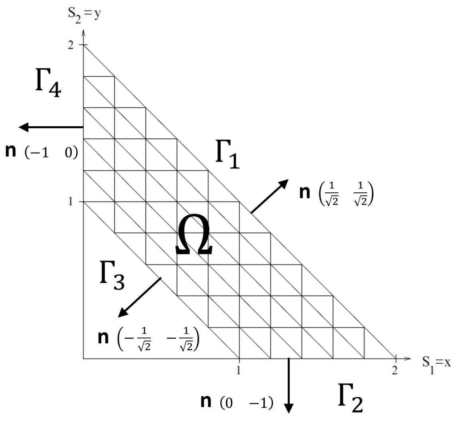
2. Integral Representation Formula of the Solution for Options without Barriers

By the Green’s theorem, we prove the integral representation formula for the solution of the differential model problem (1) describing the value of an option V ( S 1 , S 2 , t ) based on two assets S 1 , S 2 during the time interval [ 0 , T ] .
We recall the notion of joint transition probability density function G ( S 1 , S 2 , t ; S ˜ 1 , S ˜ 2 , t ˜ ) (also known as Green’s or fundamental solution) from the classical theory of PDEs [13]: denoting the space differential operator by
L [ V ] : = σ 1 2 S 1 2 2 2 V S 1 2 + r S 1 V S 1 + σ 2 2 S 2 2 2 2 V S 2 2 + r S 2 V S 2 + ρ σ 1 σ 2 S 1 S 2 2 V S 1 S 2 r V ,
G is solution of (1), i.e.,
G t ( S 1 , S 2 , t ) + L [ G ] ( S 1 , S 2 , t ) = 0
w.r.t. the first tern of variables and of the adjoint model problem (4) and (5) w.r.t. the second tern of variables:
G t ˜ ( S ˜ 1 , S ˜ 2 , t ˜ ) + L [ G ] ( S ˜ 1 , S ˜ 2 , t ˜ ) = 0 ( S ˜ 1 , S ˜ 2 , t ˜ ) R + × R + × t , +
G ( S 1 , S 2 , t ; S ˜ 1 , S ˜ 2 , t ˜ ) = δ ( S 1 , S ˜ 1 ) δ ( S 2 , S ˜ 2 ) ( S ˜ 1 , S ˜ 2 ) R + × R + ;
moreover it is such that
( L [ V ] , G ) = ( V , L [ G ] )
having set ( · , · ) the standard L 2 scalar product. The adjoint operator L is defined as
L [ G ] : = σ 1 2 S ˜ 1 2 2 2 G S ˜ 1 2 + G S ˜ 1 ( r S ˜ 1 + 2 σ 1 2 S ˜ 1 + ρ σ 1 σ 2 S ˜ 1 ) + σ 2 2 S ˜ 2 2 2 2 G S ˜ 2 2 + G S ˜ 2 ( r S ˜ 2 + 2 σ 2 2 S ˜ 2 + ρ σ 1 σ 2 S ˜ 2 ) + ρ σ 1 σ 2 S ˜ 1 S ˜ 2 2 G S ˜ 1 S ˜ 2 + G ( ρ σ 1 σ 2 3 r + σ 1 2 + σ 2 2 ) .
From [14] the fundamental solution is known to be
G ( S 1 , S 2 , t ; S ˜ 1 , S ˜ 2 , t ˜ ) = e r ( t ˜ t ) 2 π ( t ˜ t ) exp α Σ 1 α 2 σ 1 σ 2 S ˜ 1 S ˜ 2 det Σ
with
α i = log S i S ˜ i + r σ i 2 2 ( t ˜ t ) σ i t ˜ t , i = 1 , 2
the elements of the array α and
Σ = 1 ρ 12 ρ 12 1 .
the correlation matrix.
Proposition 1.
The fundamental solution (8) of (3)–(5) verifies, t ˜ , t [ 0 , T ] , the following identities
I 1 : = R + × R + G ( S 1 , S 2 , t ; S ˜ 1 , S ˜ 2 , t ˜ ) d S ˜ 1 d S ˜ 2 = e r ( t ˜ t )
I 2 : = R + × R + G ( S 1 , S 2 , t ; S ˜ 1 , S ˜ 2 , t ˜ ) d S 1 d S 2 = e ( t ˜ t ) ( 3 r σ 1 σ 2 ρ 12 σ 1 2 σ 2 2 )
Proof. 
From (8),
G ( S 1 , S 2 , t ; S ˜ 1 , S ˜ 2 , t ˜ ) = e r ( t ˜ t ) 2 π ( t ˜ t ) exp α 1 2 + α 2 2 2 α 1 α 2 ρ 12 2 ( 1 ρ 12 2 ) σ 1 σ 2 S ˜ 1 S ˜ 2 1 ρ 12 2
hence
I 1 = e r ( t ˜ t ) 2 π ( t ˜ t ) σ 1 σ 2 1 ρ 12 2 R + exp α 1 2 2 ( 1 ρ 12 2 ) S ˜ 1 d S ˜ 1 R + exp α 2 2 2 α 1 α 2 ρ 12 2 ( 1 ρ 12 2 ) S ˜ 2 d S ˜ 2
by the changes of variables ξ i : = log ( S ˜ i ) and exploiting the property 0 + e ξ 2 d ξ = π / 2 , we obtain
= e r ( t ˜ t ) 2 π ( t ˜ t ) σ 1 σ 2 1 ρ 12 2 R + e α 1 2 2 2 π σ 2 2 ( t ˜ t ) ( 1 ρ 12 2 ) d ξ 1 = e r ( t ˜ t ) 2 π ( t ˜ t ) σ 1 R + e α 1 2 2 d ξ 1 = e r ( t ˜ t ) .
Analogously
I 2 = e r ( t ˜ t ) 2 π ( t ˜ t ) σ 1 σ 2 S ˜ 1 S ˜ 2 1 ρ 12 2 R + e α 1 2 2 ( 1 ρ 12 2 ) d S 1 R + e α 2 2 2 α 1 α 2 ρ 12 2 ( 1 ρ 12 2 ) d S 2 = e ( t ˜ t ) ( 2 r + σ 2 2 ρ 12 2 σ 2 2 2 ) 2 π ( t ˜ t ) σ 1 S ˜ 1 R + e α 1 2 2 + α 1 ρ 12 ( t ˜ t ) σ 2 d S 1 = e ( t ˜ t ) ( 3 r + σ 2 2 + σ 1 2 + σ 1 σ 2 ρ 12 )
   □
Remark 1.
Note that I 1 and I 2 turn out to coincide with the coefficients of the changes of variables G ˜ = e r ( t ˜ t ) G and G ˜ = e ( 3 r σ 1 σ 2 ρ 12 σ 1 2 σ 2 2 ) ( t ˜ t ) G allowing to obtain (3) and (4), respectively, without the last term.
With the knowledge of the fundamental solution, we will derive, by mathematical analysis tools, the following integral representation formula:
Proposition 2.
The Feynman–Kac formula
V ( S 1 , S 2 , t ) = R + × R + V ( S ˜ 1 , S ˜ 2 , T ) G ( S 1 , S 2 , t ; S ˜ 1 , S ˜ 2 , T ) d S ˜ 1 d S ˜ 2
giving the option value as expected value of the payoff function, holds.
Proof. 
Multiply (1) by G and integrate in time-space domain
0 = t T R + × R + V t ˜ ( S ˜ 1 , S ˜ 2 , t ˜ ) G ( S 1 , S 2 , t ; S ˜ 1 , S ˜ 2 , t ˜ ) d t ˜ d S ˜ 1 d S ˜ 2 + t T R + × R + L [ V ] ( S ˜ 1 , S ˜ 2 , t ˜ ) G ( S 1 , S 2 , t ; S ˜ 1 , S ˜ 2 , t ˜ ) d t ˜ d S ˜ 1 d S ˜ 2
then, integrating by parts in time and in space and applying (6), one obtains
= R + × R + V ( S ˜ 1 , S ˜ 2 , T ) G ( S 1 , S 2 , t ; S ˜ 1 , S ˜ 2 , T ) d S ˜ 1 d S ˜ 2 R + × R + V ( S ˜ 1 , S ˜ 2 , t ) G ( S 1 , S 2 , t ; S ˜ 1 , S ˜ 2 , t ) d S ˜ 1 d S ˜ 2 t T R + × R + V ( S ˜ 1 , S ˜ 2 , t ˜ ) G t ˜ ( S 1 , S 2 , t ; S ˜ 1 , S ˜ 2 , t ˜ ) d t ˜ d S ˜ 1 d S ˜ 2 + t T R + × R + V ( S ˜ 1 , S ˜ 2 , t ˜ ) L [ G ] ( S 1 , S 2 , t ; S ˜ 1 , S ˜ 2 , t ˜ ) d t ˜ d S ˜ 1 d S ˜ 2
= R + × R + V ( S ˜ 1 , S ˜ 2 , T ) G ( S 1 , S 2 , t ; S ˜ 1 , S ˜ 2 , T ) d S ˜ 1 d S ˜ 2 R + × R + V ( S ˜ 1 , S ˜ 2 , t ) δ ( S 1 , S ˜ 1 ) δ ( S 2 , S ˜ 2 ) d S ˜ 1 d S ˜ 2 t T R + × R + V ( S ˜ 1 , S ˜ 2 , t ˜ ) G t ˜ L [ G ] ( S 1 , S 2 , t ; S ˜ 1 , S ˜ 2 , t ˜ ) d t ˜ d S ˜ 1 d S ˜ 2
and then, thanks to property (6), these steps lead to the Feynman-Kac formula.    □

3. Integral Representation Formula of the Solution for Barrier Options

If we consider barrier options, sometimes analytical solutions are known (some examples are collected in [15]) but sometimes not. For example, in [12], the author considers the case of a European-style two-assets-basket double-barrier call option with payoff
V ( S 1 , S 2 , T ) = max ( S 1 + S 2 K , 0 )
and two knock-out barrier conditions
V ( S 1 , S 2 , T ) = 0 S 1 + S 2 B 1
V ( S 1 , S 2 , T ) = 0 S 1 + S 2 B 2
with down-and-out barrier B 1 and up-and-out barrier B 2 . Then, the resulting domain Ω is partitioned as shown in Figure 1 in order to approximate the option value by a Finite Element Method.
However, if we are interested in the computation of the option value only at a desired point ( S 1 , S 2 ) of the domain, it may certainly be convenient to apply the strategy already tested for various kind of options (based on one asset only) under several dynamics [2,3,4,5,16,17] and that we called SABO.
The method is based on a new analytical representation formula whose proof relies on Green’s Theorem and retraces the proof of Feynman–Kac formula.
Proposition 3.
The solution of problem (1), (13) and (14), ( S 1 , S 2 , t ) Ω R 2 × [ 0 , T ) , can be expressed by the following integral representation formula:
V ( S 1 , S 2 , t ) = Ω V ( S ˜ 1 , S ˜ 2 , T ) G ( S 1 , S 2 , t ; S ˜ 1 , S ˜ 2 , T ) d S ˜ 1 d S ˜ 2 + t T Ω φ ( S ˜ 1 , S ˜ 2 , t ˜ ) d t ˜ d S ˜ 1 d S ˜ 2
with the functional φ defined in (17) below.
Proof. 
Multiply (1) by G and integrate in time and in the domain Ω
0 = t T Ω V t ˜ ( S ˜ 1 , S ˜ 2 , t ˜ ) G ( S 1 , S 2 , t ; S ˜ 1 , S ˜ 2 , t ˜ ) d t ˜ d S ˜ 1 d S ˜ 2 + t T Ω L [ V ] ( S ˜ 1 , S ˜ 2 , t ˜ ) G ( S 1 , S 2 , t ; S ˜ 1 , S ˜ 2 , t ˜ ) d t ˜ d S ˜ 1 d S ˜ 2
then, integrating by parts in time and applying Green’s Theorem and (6), one obtains
= Ω V ( S ˜ 1 , S ˜ 2 , T ) G ( S 1 , S 2 , t ; S ˜ 1 , S ˜ 2 , T ) d S ˜ 1 d S ˜ 2 Ω V ( S ˜ 1 , S ˜ 2 , t ) G ( S 1 , S 2 , t ; S ˜ 1 , S ˜ 2 , t ) d S ˜ 1 d S ˜ 2 t T Ω V ( S ˜ 1 , S ˜ 2 , t ˜ ) G t ˜ ( S 1 , S 2 , t ; S ˜ 1 , S ˜ 2 , t ˜ ) d t ˜ d S ˜ 1 d S ˜ 2 + t T Ω V ( S ˜ 1 , S ˜ 2 , t ˜ ) L [ G ] ( S 1 , S 2 , t ; S ˜ 1 , S ˜ 2 , t ˜ ) d t ˜ d S ˜ 1 d S ˜ 2 + t T Ω p ( S 1 , S 2 , t ; S ˜ 1 , S ˜ 2 , t ˜ ) · n d t ˜ d S ˜ 1 d S ˜ 2
having defined Ω as the boundary of the domain, n as its unit normal vector outwardly directed and p = ( p 1 , p 2 ) as
p 1 = 1 2 σ 1 2 S ˜ 1 2 G V S ˜ 1 V G S ˜ 1 + 1 2 ρ σ 1 σ 2 S ˜ 1 S ˜ 2 G V S ˜ 2 V G S ˜ 2 V G σ 1 2 S ˜ 1 + 1 2 ρ σ 1 σ 2 S ˜ 1 r S ˜ 1 p 2 = 1 2 σ 2 2 S ˜ 2 2 G V S ˜ 2 V G S ˜ 2 + 1 2 ρ σ 1 σ 2 S ˜ 1 S ˜ 2 G V S ˜ 1 V G S ˜ 1 V G σ 2 2 S ˜ 2 + 1 2 ρ σ 1 σ 2 S ˜ 2 r S ˜ 2 .
Thus we can conclude that
0 = Ω V ( S ˜ 1 , S ˜ 2 , T ) G ( S 1 , S 2 , t ; S ˜ 1 , S ˜ 2 , T ) d S ˜ 1 d S ˜ 2 Ω V ( S ˜ 1 , S ˜ 2 , t ) δ ( S 1 , S ˜ 1 ) δ ( S 2 , S ˜ 2 ) d S ˜ 1 d S ˜ 2 t T Ω V ( S ˜ 1 , S ˜ 2 , t ˜ ) G t ˜ L [ G ] ( S 1 , S 2 , t ; S ˜ 1 , S ˜ 2 , t ˜ ) d t ˜ d S ˜ 1 d S ˜ 2 + t T Ω φ ( S 1 , S 2 , t ; S ˜ 1 , S ˜ 2 , t ˜ ) d t ˜ d S ˜ 1 d S ˜ 2
with
φ ( S 1 , S 2 , t ; S ˜ 1 , S ˜ 2 , t ˜ ) = p ( S 1 , S 2 , t ; S ˜ 1 , S ˜ 2 , t ˜ ) · n
   □
Remark 2.
The representation formula, and SABO in general, can be naturally adapted to barrier options configurations different from the proposed example. Note also that it is not really important to know exactly the expression of the functional φ because, as it depends on the unknown solution V, it is unknown in its turn and therefore it will be numerically determined.
Remark 3.
The representation formula can be analytically derived in time or in space to obtain Greeks functions that can be straightforwardly evaluated by SABO without the need of evaluating option values (look at [2]).
In the example (12)–(14), due to the configuration of the boundary Ω = Γ 1 Γ 2 Γ 3 Γ 4 (see Figure 1), the integral of φ reduces to
t T Ω φ ( S 1 , S 2 , t ; S ˜ 1 , S ˜ 2 , t ˜ ) d t ˜ d S ˜ 1 d S ˜ 2 = t T Γ 1 Γ 3 φ ( S 1 , S 2 , t ; S ˜ 1 , S ˜ 2 , t ˜ ) d t ˜ d S ˜ 1 d S ˜ 2
because on Γ 2 : = ( S 1 , 0 ) : B 1 S 1 B 2 the first component of the normal vector is null and every term of p 2 has the factor S 2 , trivial on Γ 2 ; on Γ 4 : = ( 0 , S 2 ) : B 1 S 2 B 2 the second component of the normal vector is null and every term of p 1 has the factor S 1 , trivial on Γ 4 .
Moreover, considering double knock-out barriers on Γ 1 : = ( S 1 , S 2 ) : S 1 + S 2 = B 2 and on Γ 3 : = ( S 1 , S 2 ) : S 1 + S 2 = B 1 , the option value V is equal to 0, justifying the representation formula: ( S 1 , S 2 , t ) Ω × [ 0 , T )
V ( S 1 , S 2 , t ) = Ω V ( S ˜ 1 , S ˜ 2 , T ) G ( S 1 , S 2 , t ; S ˜ 1 , S ˜ 2 , T ) d S ˜ 1 d S ˜ 2 + t T Γ 1 Γ 3 G ( S 1 , S 2 , t ; S ˜ 1 , S ˜ 2 , t ˜ ) ϕ ( S ˜ 1 , S ˜ 2 , t ˜ ) d t ˜ d S ˜ 1 d S ˜ 2
with ϕ depending only on ( S ˜ 1 , S ˜ 2 , t ˜ ) Γ 1 Γ 3 × [ 0 , T ) , i.e.,
ϕ ( S ˜ 1 , S ˜ 2 , t ˜ ) = 1 2 σ 1 2 S ˜ 1 2 V S ˜ 1 + 1 2 ρ σ 1 σ 2 S ˜ 1 S ˜ 2 V S ˜ 2 n 1 + 1 2 σ 2 2 S ˜ 2 2 V S ˜ 2 + 1 2 ρ σ 1 σ 2 S ˜ 1 S ˜ 2 V S ˜ 1 n 2 .

4. Boundary Integral Equation

The representation Formula (18) of V holds in the whole domain and can be used once the unknown density ϕ is recovered. To this aim, the idea is to consider the application of the representation formula at the barriers, where ( S 1 , S 2 , t ) Γ 1 Γ 3 × [ 0 , T ) the option value is trivial, i.e., V ( S 1 , S 2 , t ) = 0 and therefore
t T Γ 1 Γ 3 G ( S 1 , S 2 , t ; S ˜ 1 , S ˜ 2 , t ˜ ) ϕ ( S ˜ 1 , S ˜ 2 , t ˜ ) d t ˜ d S ˜ 1 d S ˜ 2 = Ω V ( S ˜ 1 , S ˜ 2 , T ) G ( S 1 , S 2 , t ; S ˜ 1 , S ˜ 2 , T ) d S ˜ 1 d S ˜ 2 .
This Boundary Integral Equation (BIE) in the unknown ϕ is a Volterra integral equation of first kind and can be numerically solved as described in the following section.
Remark 4.
This strategy can be extended to higher dimensions, denoting by Γ the hyperplane defined by the barrier conditions. The representation formula still holds: ( S 1 , , S n , t ) Ω × [ 0 , T )
V ( S 1 , , S n , t ) = Ω V ( S ˜ 1 , , S ˜ n , T ) G ( S 1 , , S n , t ; S ˜ 1 , , S ˜ n , T ) d S ˜ 1 d S ˜ n + t T Γ G ( S 1 , , S n , t ; S ˜ 1 , , S ˜ n , t ˜ ) ϕ ( S ˜ 1 , , S ˜ n , t ˜ ) d t ˜ d S ˜ 1 d S ˜ n
together with the BIE with knock-out condition: ( S 1 , S 2 , t ) Γ × [ 0 , T )
t T Γ G ( S 1 , , S n , t ; S ˜ 1 , , S ˜ n , t ˜ ) ϕ ( S ˜ 1 , , S ˜ n , t ˜ ) d t ˜ d S ˜ 1 , , d S ˜ n = Ω V ( S ˜ 1 , , S ˜ n , T ) G ( S 1 , , S n , t ; S ˜ 1 , , S ˜ n , T ) d S ˜ 1 d S ˜ 2
and with the general expression of fundamental solution G written in [14].
Remark 5.
If the asset domain is either a 2 or 3 or 4 dimensional domain, to solve (21) means to reduce the dimensionality of the problem by one. In this case, the collocation method can be implemented, as proposed in Section 5 (introducing suitable mesh triangulations), since finite element discretization can be easily applied up to three dimensions with presumably greater accuracy w.r.t. Monte Carlo simulations. However, of course, the collocation method suffers the curse of dimensionality. Therefore, first of all, SABO in this framework, is suggested as an alternative to deterministic methods (finite difference methods and finite element methods) for its higher efficiency.
With the increasing of the dimension n > 4 , (21) is still valid and very general, not requiring special conditions as for example in [18], so the strategy of solving (21) can be anyway taken into account. An idea could be to involve Monte Carlo method, not as a method for path simulation [9], but considered as a quadrature method [19] directly applied to the integral terms in (21). Then unknown ϕ might be represented by linear combination of radial basis functions around some nodes spread out in the n 1 -dimensional hyperplane Γ. This will be the subject of future investigation.

5. Numerical Approximation by Collocation BEM

We introduce
ϕ ˜ ( S 1 , S 2 , t ) : = n = 1 N Δ t m = 1 M Δ S α n m ϕ ¯ m ( S 1 , S 2 ) ϕ ^ n ( t )
for the numerical approximation of ϕ by:
  • piecewise constant functions in time
    ϕ ^ n ( t ) : = H [ t t n 1 ] H [ t t n ] n = 1 , , N Δ t
    defined by the Heaviside functions H [ · ] on a uniform decomposition of the time interval [ 0 , T ] :
    Δ t = T N Δ t , N Δ t N + t n = n N Δ t , n = 0 , , N Δ t ,
  • piecewise constant functions in space ϕ ¯ m ( S ) = ϕ ¯ m ( S 1 , S 2 ) , m = 1 , , M ¯ Δ S , M ¯ Δ S + 1 , , M Δ S defined on a decomposition T 1 = { e 1 , , e M ¯ Δ S } on Γ 1 and T 2 = { e M ¯ Δ S + 1 , , e M Δ S } on Γ 2 constituted by M Δ S segments such that length ( e i ) Δ S with e i e j = if i j
The related unknown array
α = α ( 1 ) α ( 1 ) α ( 2 ) α ( N Δ t ) α ( ) = α 1 , , α M Δ S , = 1 , , N Δ t
can be computed by solving a linear system
M α = β ,
of N Δ t × M Δ S equations obtained by collocating the BIE (19) at the midpoints of time decomposition interval
t ¯ n = t n 1 + t n 2 , n = 1 , , N Δ t
and at the midpoints of space decomposition segments
S ¯ m = ( S ¯ 1 ( m ) , S ¯ 2 ( m ) ) , m = 1 , , M Δ S .
Note that the matrix M has a block upper triangular Toeplitz structure
M ( 1 ) M ( 2 ) M ( 3 ) M ( N Δ t ) 0 M ( 1 ) M ( 2 ) M ( N Δ t 1 ) 0 0 M ( 1 ) M ( N Δ t 2 ) 0 0 0 M ( 1 )
and this is due to the form of the fundamental solution (8): the starting PDE Equation (1) has coefficients independent of time implying that the fundamental solution depends on time only through the difference t ˜ t and, by consequence, each block depends only on t n t ¯ n . From the computational point of view, this means notable computational and memory savings because only the last column of blocks needs to be computed and the linear system (23) can be solved by block-backward substitution
z ( ) = β ( ) j = 2 N Δ t + 1 M ( j ) α ( + j 1 ) M ( 1 ) α ( ) = z ( ) . = N Δ t , , 1
where only the non singular block M ( 1 ) needs to be inverted.
We can get the expression of a general entry of the matrix block M ( ) , = 1 , , N Δ t , introducing, in the lhs of (19), a space-time piecewise constant approximation (22) and collocation points (24) and (25): m ¯ , m = 1 , M Δ S , n ¯ = 1 , N Δ t , n = n ¯ , N Δ t
M m ¯ m ( ) = M m ¯ m n ¯ n = M m ¯ m ( n n ¯ + 1 ) = t ¯ n ¯ T e m G ( S ¯ 1 ( m ¯ ) , S ¯ 2 ( m ¯ ) , t ¯ n ¯ ; S ˜ 1 , S ˜ 2 , t ˜ ) ϕ ¯ m ( S ˜ 1 , S ˜ 2 ) ϕ ^ n ( t ˜ ) d t ˜ d S ˜ 1 d S ˜ 2 = max ( t n 1 , t ¯ n ¯ ) t n e m G ( S ¯ 1 ( m ¯ ) , S ¯ 2 ( m ¯ ) , t ¯ n ; S ˜ 1 , S ˜ 2 , t ˜ ) d t ˜ d S ˜ 1 d S ˜ 2
and, collocating the rhs of (19) in the same way, we can write
β m ¯ = β m ¯ n ¯ = Ω V ( S ˜ 1 , S ˜ 2 , T ) G ( S ¯ 1 ( m ¯ ) , S ¯ 2 ( m ¯ ) , t ¯ n ¯ ; S ˜ 1 , S ˜ 2 , T ) d S ˜ .
Once the array α of coefficients in (22) are computed by solving the linear system (23), the unknown functional ϕ in (18) can be replaced by its approximation ϕ ˜ , in order to get the approximation of the option price, at the desired time instant and assets values, without the need of introducing grids or triangulation over the domain Ω as in Figure 1.
Note that the evaluation of system entries can be simply performed by Matlab®integral2” function as it presents only little troubles: the degeneration of the fundamental solution in time towards the Dirac delta distribution when t t ˜ (look at (5)) and possible non-smoothness of the payoff function like, for example, in the case of Basket options.

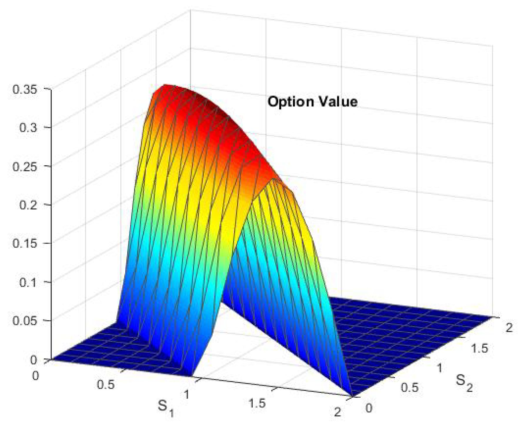
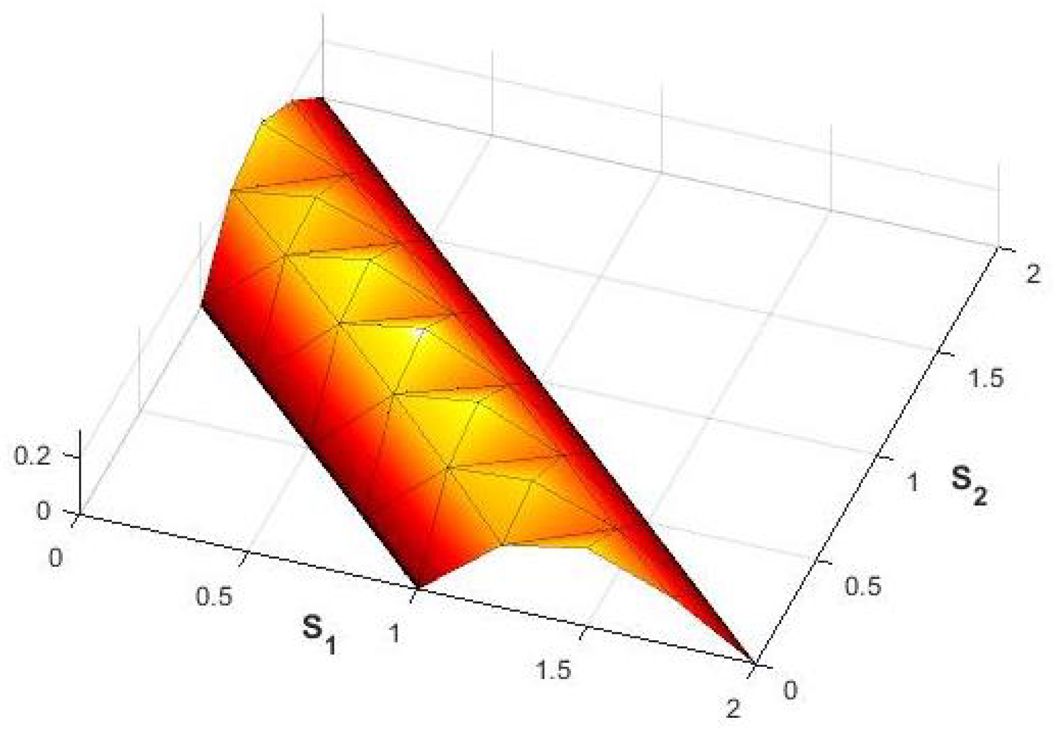
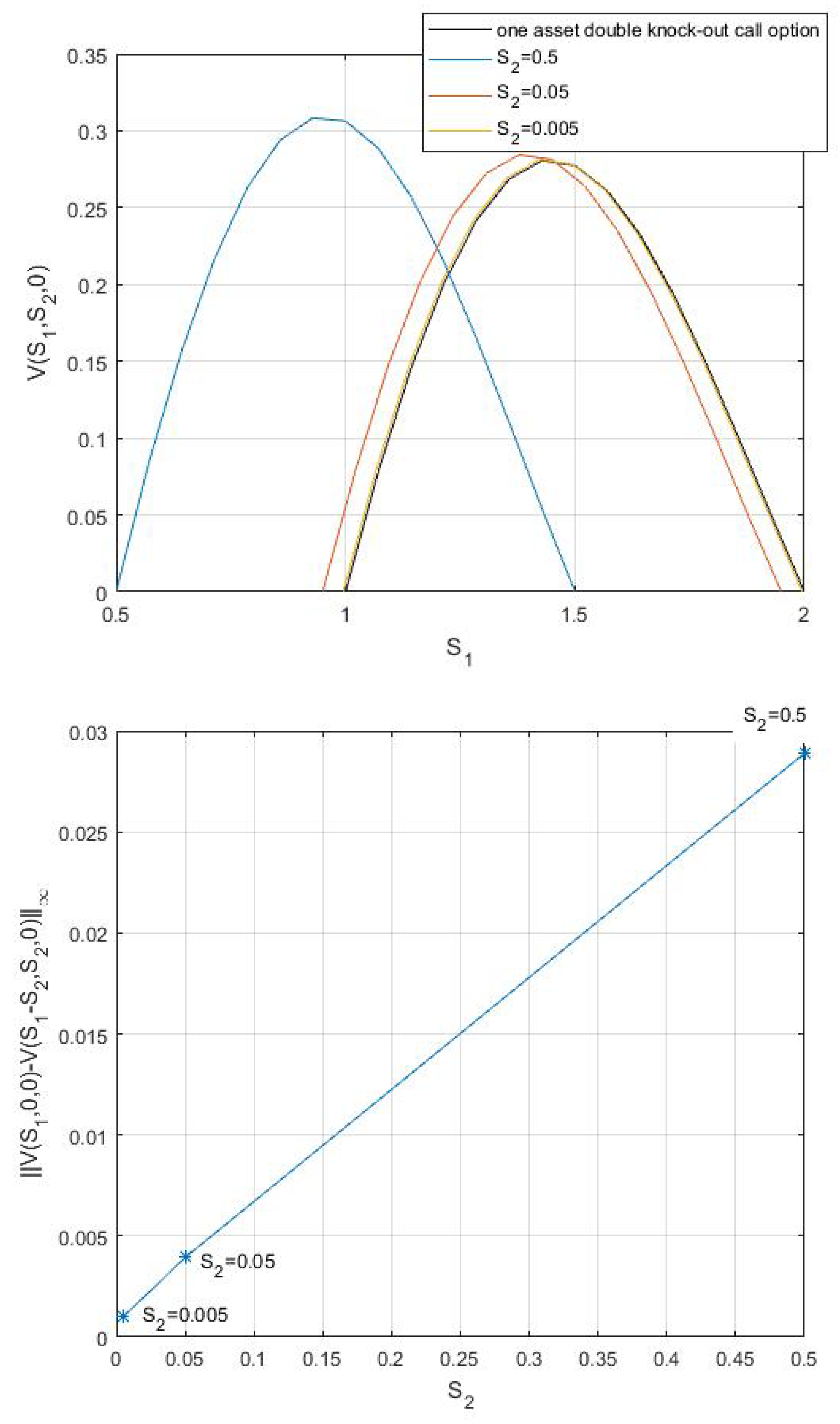
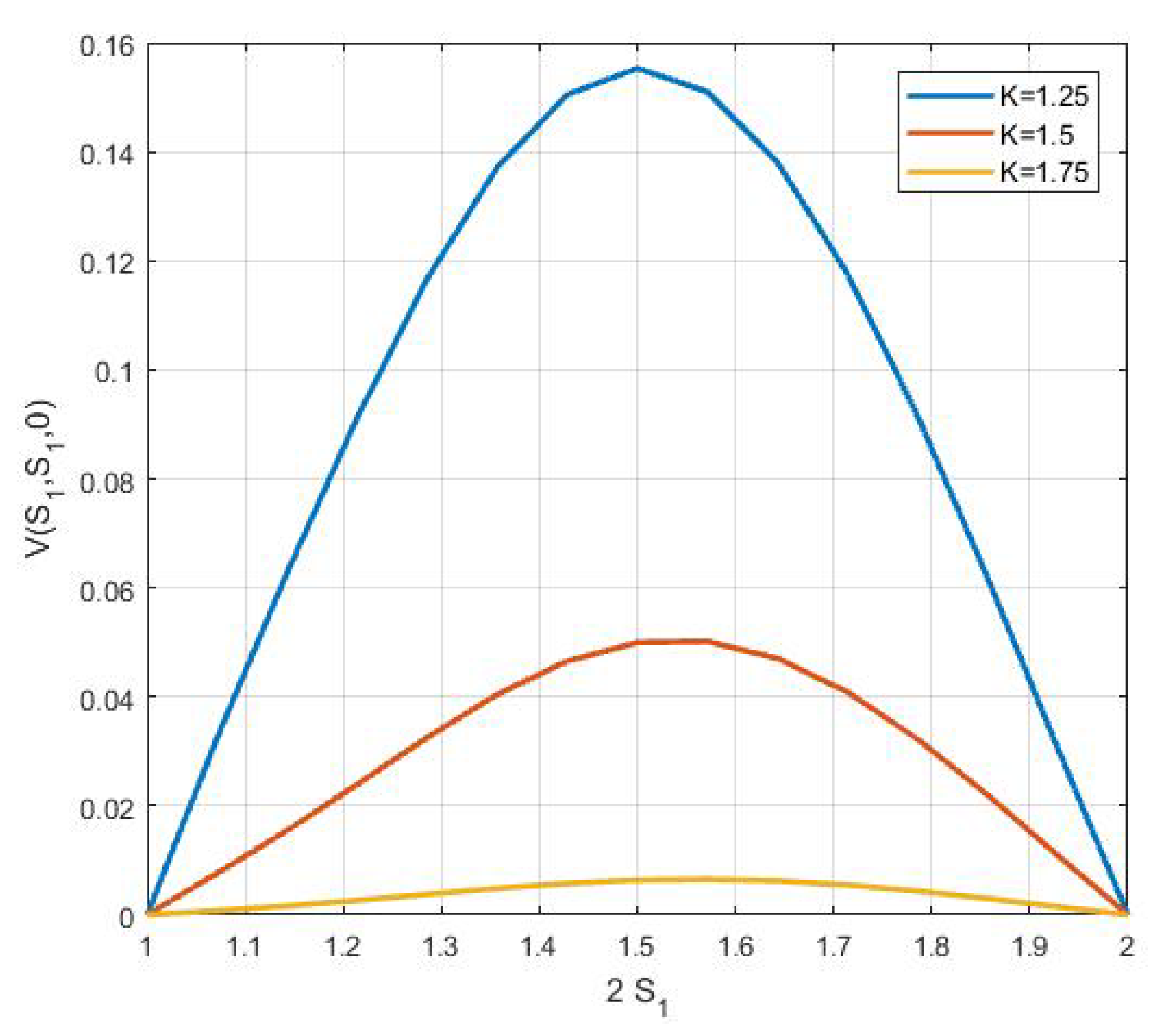
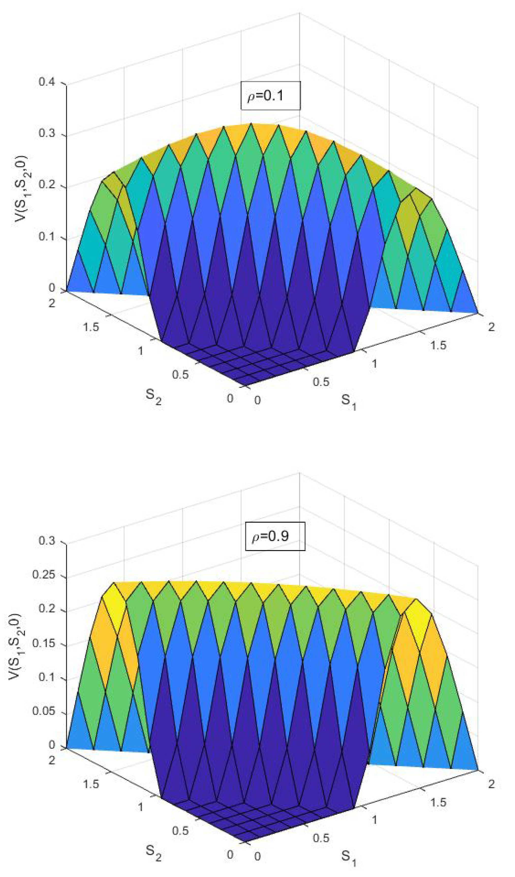
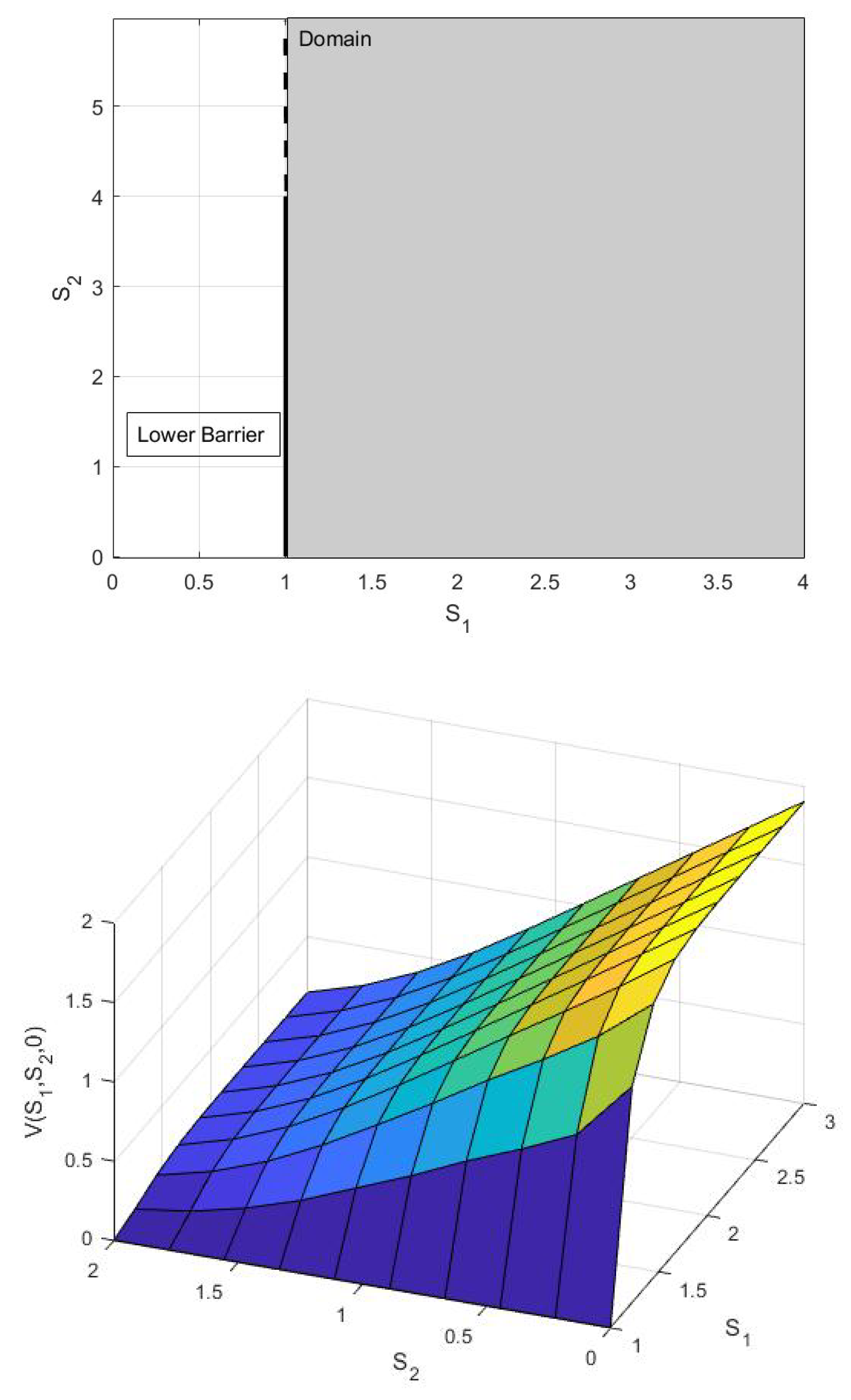
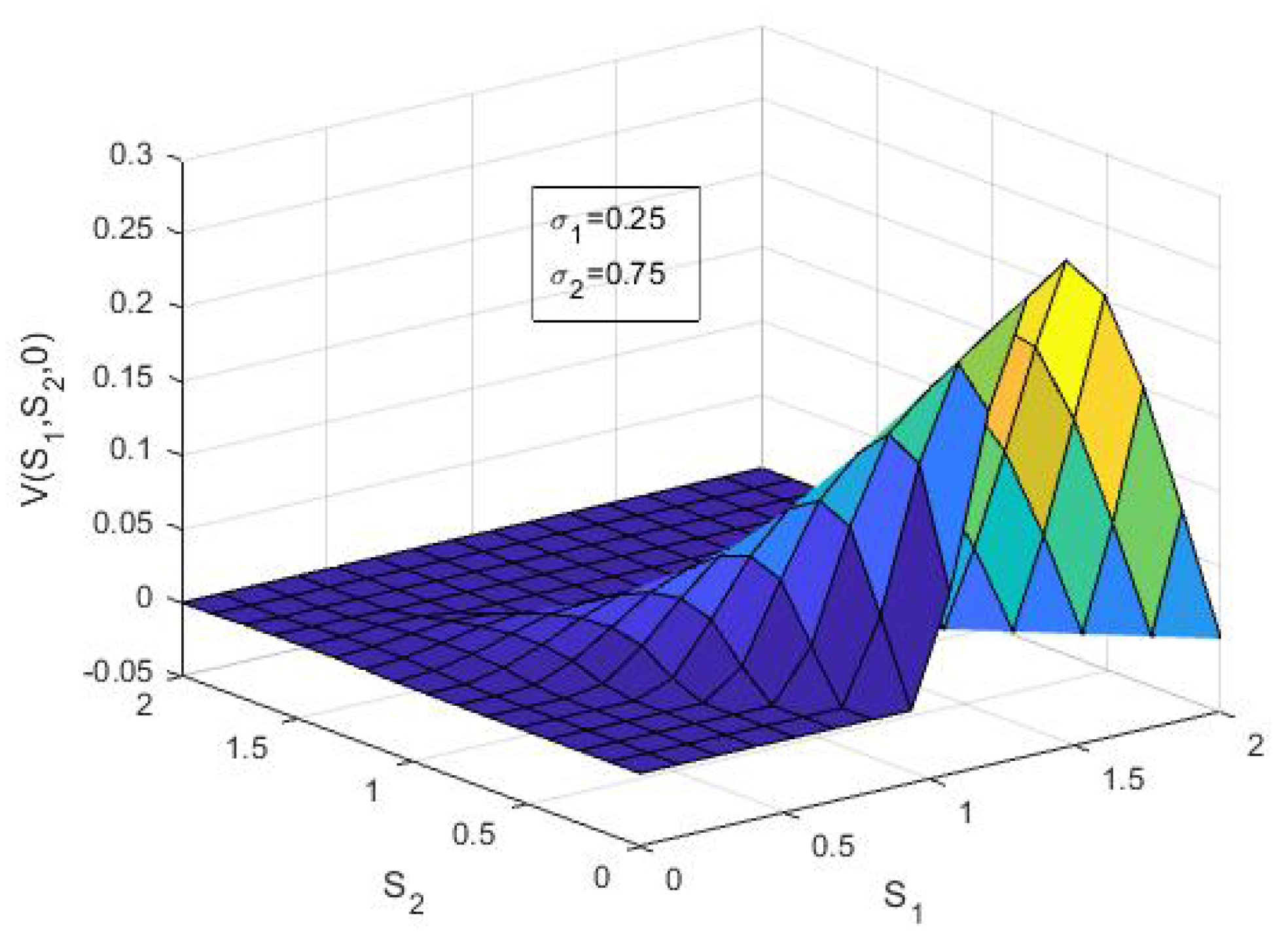
6. Numerical Results and Discussion

Consider the problem (1), (12), (13) and (14) of evaluating a double knock-out basket call option based on two assets
V ( S 1 , S 2 , T ) = max ( S 1 + S 2 K , 0 )
with data suggested in [12] and listed in Table 1. The domain is as depicted in Figure 1. Numerical results have been obtained by the code inserted in the Appendix A.
The approximated solution, represented in Figure 2, is evaluated over a rectangular grid of points, vertices of 16 2 simplices that subdivide the square [ 0 , 2 ] 2 . It is obtained by SABO with Δ S = 0.125 2 and Δ t = 0.1 . The behavior of the solution is in good agreement with that found in [12] (“Courtesy of A. Kvetnaia”), there approximated by Finite Element Method (FEM) after having transformed Equation (1) in a divergence-free form, not necessary or useful to apply SABO.
The greater accuracy, implying greater velocity, of SABO w.r.t. Finite Differences and Monte Carlo Methods has been already highlighted in our papers about barrier options, see for example [3,20]. Here, in Table 2, we compare the CPU time of computation (Laptop computer: CPU Intel i5, 4 Gb RAM.) of SABO w.r.t. FEM as applied in [12], i.e., linear finite elements in space coupled with Crank–Nicolson scheme in time: the chosen reference value is V ( 0.5 , 1 , 0 ) = 0.306264 , obtained by stressing the discretization parameters in our SABO code ( M Δ S = N Δ t = 30 , tolerance on integrals computation equal to 10 12 ) and both methods converge towards it. The starting space mesh for FEM, that will be denoted by R 0 from now on, is made by 48 uniform triangles as depicted in Figure 3, then any successive refinement, R i i = 1 , 2 , 3 , is obtained by dividing each triangle in four uniform triangles (by connecting the midpoints of the edges). Despite not having implemented a parallel code for the computation of independent blocks in (26), SABO allows to achieve the same accuracy of FEM with a computation time of at least one lower order of magnitude.
In order to quantitatively check the reliability of numerical results, we show in Figure 4 that the approximated solution evaluated inside the domain but moving towards boundary Γ 4 (or equivalently Γ 2 ) converges to the exact solution of a double knock-out call option with the same financial parameters but based on one asset, whose explicit expression C ( S 1 , t ) can be found in [21] and is here reported for reader’s convenience:
C ( S , t ) = S n = B 2 n B 1 n 2 r σ 2 + 1 N [ d 1 ] N [ d 2 ] B 1 n + 1 B 2 n S 2 r σ 2 + 1 N [ d 3 ] N [ d 4 ] K e r ( T t ) n = B 2 n B 1 n 2 r σ 2 1 N [ d 1 σ T t ] N [ d 2 σ T t ] B 1 n + 1 B 2 n S 2 r σ 2 1 N [ d 3 σ T t ] N [ d 4 σ T t ]
d 1 = ln S B 2 2 n K B 1 2 n + r + σ 2 2 ( T t ) σ T t d 2 = ln S B 2 2 n 1 B 1 2 n + r + σ 2 2 ( T t ) σ T t d 3 = ln B 1 2 n + 2 K S B 2 2 n + r + σ 2 2 ( T t ) σ T t d 4 = ln B 1 2 n + 2 S B 2 2 n + 1 + r + σ 2 2 ( T t ) σ T t
with N the standard normal cumulative distribution function.
These “boundary conditions” on Γ 2 and Γ 4 are necessary to apply Finite Element Method; on the contrary, they are not set during SABO implementation, but they are naturally matched by the approximated solution.
In order to show the stability of results we have changed also some financial parameters starting from Table 1: in Figure 5, the value of the strike price (on the top) and the volatility of one asset (on the bottom) and, in Figure 6, the correlation (poorly correlated assets with ρ = 0.1 on the top, highly correlated assets with ρ = 0.9 on the bottom).
Consider a put down and out option based on two assets whose value is the solution of (1) provided with the payoff function
V ( S 1 , S 2 , T ) = max ( K S 2 , 0 ) if S 1 [ B , + ]
meaning that there is a lower out barrier on the first asset only. The boundary and the domain are shown in Figure 7 top.
In Figure 7 bottom, there is the representation of the approximated solution at time t = 0 , obtained with M Δ S = N Δ t = 10 . In Table 3, we can observe the stabilization of digits in the numerical approximation of V ( S 1 , S 2 , 0 ) at ( S 1 , S 2 ) = ( 2 , 1 ) doubling the number of discretization nodes M Δ S and N Δ t in (22).

7. Conclusions

In this paper, we have extended the SABO method, based on collocation BEM, for pricing barrier options depending on two assets. The good performance of this technique, largely employed in the past for options on a single asset, has been shown by means of numerical results. The implemented Matlab® code is enclosed in the Appendix A, in such a way that it can be directly used by any interested reader.

Author Contributions

All authors contributed equally to this work. All authors have read and agreed to the published version of the manuscript.

Funding

This work has been partially supported by INdAM-GNCS Research Projects.

Conflicts of Interest

The authors declare no conflict of interest.

Appendix A. Matlab® Code

All the above provided numerical results were obtained by codes developed with Matlab® Release 2007b running on a laptop computer (CPU Intel i5, 4 Gb RAM). The one implementing SABO algorithm applied to the first numerical example in this paper is below available.
  • %Basket options
  • %Code for the example with data taken from the book of R. Seydel
  • close all
  • clear
  • clc
  • %%%%%%%%%%%%%%%%%%%%%%%%%%%%%%%
  • global r sigma1 sigma2 rho
  • %financial parameters
  • B2=2; %50; %upper barrier
  • B1=1; %0.1; %lower barrier
  • T=1; %expiry
  • r=0.05; %interest rate
  • sigma1=0.25; %volatility of S1
  • sigma2=0.25; %volatility of S2
  • rho=0.7; %correlation
  • K=1; %1.5; %strike price
  • if K>=B2
  •     disp(’strike > upper barrier −> option value = 0’)
  •     return
  • end
  • %%%%%%%%%%%%%%%%%%%%%%%%%%%%%%%
  • %discretization in space
  • tol=10^−12;
  • epsi=10^−10;
  • L1=B2∗sqrt(2); %length of Gamma1
  • L3=B1∗sqrt(2); %length of Gamma3
  • MS1=10; %n. of segments on Gamma1
  • dS1=B2/MS1;
  • MS3=ceil(B1/dS1); %n. of segments on Gamma1
  • dS3=B1/MS3;
  • L=[L1/MS1:L1 L3/MS3:L3]; %length of each segment
  • B=[B2∗ones(1,MS1) B1∗ones(1,MS3)]; %belonged barrier
  • x0=[B2:−dS1:dS1 0:dS3:B1−dS3]; %first abscissa of each segment
  • x0(MS1+1)=epsi;
  • x1=[B2−dS1:−dS1:0 dS3:dS3:B1]; %second abscissa of each segment
  • x1(MS1)=epsi;
  • y0=[0:dS1:B2−dS1 B1:−dS3:dS3]; %first ordinate of each segment
  • y0(1)=epsi;
  • y1=[dS1:dS1:B2 B1−dS3:−dS3:0]; %second ordinate of each segment
  • y1(end)=epsi;
  • xbar=[B2−dS1/2:−dS1:0 0+dS3/2:dS3:B1]; %abscissae midpoints
  • ybar=[0+dS1/2:dS1:B2 B1−dS3/2:−dS3:0]; %ordinates midpoints
  • %discretization in time
  • Nt=10; %8;
  • dt=T/Nt;
  • t=0:dt:T;
  • tbar=(t(1:end−1)+t(2:end))/2; %midpoints
  • %%%%%%%%%%%%%%%%%%%%%%%%%%%%%%%%%
  • %Matrix entries
  • disp(’Computation of the matrix entries’)
  • M=zeros(MS1+MS3,MS1+MS3,Nt);
  • %Matrix diagonal block
  • for m=1:MS1+MS3
  •     for mbar=1:MS1+MS3
  •         M(mbar,m,1)=integral2(@(tau,l)…
  •             Solfond(xbar(mbar),ybar(mbar),tbar(1),l,B(m)−l,tau),…
  •             tbar(1)+epsi,t(2),x0(m),x1(m));%,’AbsTol’,tol,’RelTol’,tol);
  •     end
  • end
  •  
  • %Other matrix blocks of the first row
  • for ell=2:Nt
  •     for m=1:MS1+MS3
  •         for mbar=1:MS1+MS3
  •             M(mbar,m,ell)=integral2(@(tau,l)…
  •                 Solfond(xbar(mbar),ybar(mbar),tbar(1),l,B(m)−l,tau),…
  •                 t(ell),t(ell+1),x0(m),x1(m));
  •         end
  •     end
  • end
  •  
  • %%%%%%%%%%%%%%%%%%%%%%%%%%%%%%%%%
  • %RHS
  • disp(’Computation of the rhs entries’)
  • MAX=max(B1,K);
  • Smin=@(S1) MAX−S1;
  • Smax=@(S1) B2−S1;
  • for ell=1:Nt
  •     for mbar=1:MS1+MS3
  •             Beta(mbar,ell)=−integral2(@(S1,S2) (S1+S2−K).∗…
  •                 Solfond(xbar(mbar),ybar(mbar),tbar(ell),S1,S2,T),…
  •                 0+epsi,MAX−epsi,Smin,Smax);
  •             Beta(mbar,ell)=Beta(mbar,ell)−…
  •                 integral2(@(S1,S2) (S1+S2−K).∗…
  •                 Solfond(xbar(mbar),ybar(mbar),tbar(ell),S1,S2,T),…
  •                 MAX,B2−epsi,0+epsi,Smax);
  •      end
  • end
  •  
  • %%%%%%%%%%%%%%%%%%%%%%%%%%%%%%%%%
  • %Linear System resolution
  • disp(’Linear System resolution’)
  • Alpha(:,Nt)=M(:,:,1)\Beta(:,Nt);
  • for ell=Nt−1:−1:1
  •     for j=2:Nt−ell+1
  •         Zeta(:,j−1)=M(:,:,j)∗Alpha(:,ell+j−1);
  •     end
  •     Alpha(:,ell)=M(:,:,1)\(Beta(:,ell)−sum(Zeta,2));
  • end
  •  
  • %%%%%%%%%%%%%%%%%%%%%%%%%%%%%%%%%
  • %Post processing at time t=0
  • disp(’Post−processing: option value’)
  • NXS1=25;
  • NXS2=25;
  • XS1=linspace(0,B2,NXS1);
  • XS2=linspace(0,B2,NXS2);
  • [X,Y]=meshgrid(XS1,XS2);
  • Value=zeros(NXS2,NXS1);
  • %Values of single asset double knock−out call on Gamma4
  • for j=1:NXS2
  •      Value(j,1)=doubleOUT_call(XS2(j),K,B1,B2,T,r,sigma2^2);
  • end
  • %Values of single asset double knock−out call on Gamma2
  • for i=1:NXS1
  •      Value(1,i)=doubleOUT_call(XS1(i),K,B1,B2,T,r,sigma1^2);
  • end
  • for i=2:NXS1
  •     for j=2:NXS2
  •         Value(j,i)=0;
  •         if(XS1(i)+XS2(j)>B1&&XS1(i)+XS2(j)<B2)
  •             Value(j,i)=integral2(@(S1,S2) (S1+S2−K).∗…
  •                 Solfond(XS1(i),XS2(j),0,S1,S2,T),…
  •                 0+epsi,MAX−epsi,Smin,Smax);
  •             Value(j,i)=Value(j,i)+…
  •                 integral2(@(S1,S2) (S1+S2−K).∗…
  •                 Solfond(XS1(i),XS2(j),0,S1,S2,T),…
  •                 MAX,B2,0+epsi,Smax);
  •             for ell=1:1:Nt
  •                 for m=1:MS1+MS3
  •                     SUM(m,ell)=Alpha(m,ell)∗integral2(@(tau,l)…
  •                         Solfond(XS1(i),XS2(j),0,l,B(m)−l,tau),…
  •                         t(ell),t(ell+1),x0(m),x1(m));
  •                 end
  •             end
  •             Value(j,i)=Value(j,i)+sum(sum(SUM,1),2);
  •         end
  •     end
  • end
  • surf(X,Y,Value)
  • xlabel(’S1’)
  • ylabel(’S2’)
  •  
  • %%%%%%%%%%%%%%%%%%%%%%%%%%%%%%%%%%%%%%%%%%%%%%%%%%%%%%%%%%%%%
  • function G=Solfond(SS1,SS2,tt,S1,S2,t)
  • % fundamental solution
  • global r sigma1 sigma2 rho
  • alpha1=(log(SS1./S1)+(r−sigma1^2/2)∗(t−tt))./(sigma1∗sqrt(t−tt));
  • alpha2=(log(SS2./S2)+(r−sigma2^2/2)∗(t−tt))./(sigma2∗sqrt(t−tt));
  • G=exp(−r∗(t−tt))./(2∗pi∗(t−tt))/sqrt(1−rho^2)/(sigma1∗sigma2)./…
  •     (S1.∗S2).∗exp(−0.5∗(alpha1.^2+alpha2.^2−2∗alpha1.∗alpha2∗rho)/…
  •     (1−rho^2));
  • end
  •  
  • %%%%%%%%%%%%%%%%%%%%%%%%%%%%%%%%%%%%%%%%%%%%%%%%%%%%%%%%%%%%%
  • function c=doubleOUT_call(S,K,L,U,t,r,sigma2)
  • % doubleOUT_call evaluates the call option with double out barrier
  • % according to the formula in Section 3 in “The complete guide to
  • % option pricing formulas” by E. G. Haug
  • %
  • % Inputs:
  • %   S: underlying asset value
  • %   K: strike price
  • %   L: lower barrier
  • %   U: upper barrier
  • %   t: time to maturity (0 not allowed!!!!!)
  • %   r: riskless interest rate
  • %   sigma2: variance of the assrt price
  • % Output:
  • %   c: value of the option at S at time t
  • %
  • if S<=L || S>=U
  •     c=0;
  • else
  •     N=5; % The sum whould be infinite, this is the approximation bound
  •  
  •     % Compute some parameters that do not change in the sum. it is therefore
  •     % convenient to compute them once for all
  •     sigma = sqrt(sigma2);
  •     m = (2∗r)/sigma2 + 1;
  •     A = (r+0.5∗sigma2)∗t;
  •     B = sigma∗sqrt(t);
  •  
  •     sum1=0;
  •     sum2=0;
  •     for ndx=−N:N
  •         % Define paramenters that change with ndx
  •         d1 = (log(S∗U^(2∗ndx)/(K∗L^(2∗ndx))) + A)./B;
  •         d2 = (log(S∗U^(2∗ndx−1)/(L^(2∗ndx))) + A)./B;
  •         d3 = (log((L^(2∗ndx+2))./(K∗S∗U^(2∗ndx))) + A)./B;
  •         d4 = (log((L^(2∗ndx+2))./(S∗U^(2∗ndx+1))) + A)./B;
  •  
  •         % Update the sums value
  •         sum1 = sum1 + (U/L)^(ndx∗m) ∗ (normcdf(d1)−normcdf(d2)) − …
  •             ((L^(ndx+1))./(S∗U^ndx)).^m .∗ (normcdf(d3)−normcdf(d4));
  •         sum2 = sum2 + (U/L)^(ndx∗(m−2)) .∗(normcdf(d1−B)−normcdf(d2−B))−…
  •             ((L^(ndx+1))./(U^ndx∗S)).^(m−2).∗(normcdf(d3−B)−normcdf(d4−B));
  •     end
  •  
  •     c = S .∗ sum1 − K∗exp(−r∗t) .∗ sum2;
  • end
  •  
  • end
  •  

References

  1. Black, F.; Scholes, M. The Pricing of Options and Corporate Liabilities. J. Political Econ. 1973, 81, 637–654. [Google Scholar] [CrossRef] [Green Version]
  2. Guardasoni, C. Semi-Analytical method for the pricing of barrier options in case of time-dependent parameters (with Matlab® codes). Commun. Appl. Ind. Math. 2018, 9, 42–67. [Google Scholar] [CrossRef] [Green Version]
  3. Guardasoni, C.; Sanfelici, S. Fast numerical pricing of barrier options under stochastic volatility and jumps. SIAM J. Appl. Math. 2016, 76, 27–57. [Google Scholar] [CrossRef]
  4. Aimi, A.; Diazzi, L.; Guardasoni, C. Efficient BEM-based algorithm for pricing floating strike Asian barrier options (with MATLAB® code). Axioms 2018, 7, 40. [Google Scholar] [CrossRef] [Green Version]
  5. Aimi, A.; Guardasoni, C. Collocation Boundary Element Method for the pricing of Geometric Asian Options. Eng. Anal. Bound. Elem. 2018, 92, 90–100. [Google Scholar] [CrossRef]
  6. Guillaume, T. On the multidimensional Black Scholes partial differential equation. Ann. Oper. Res. 2019, 281, 229–251. [Google Scholar] [CrossRef]
  7. Glasserman, P.; Staum, J. Conditioning on one-step survival for barrier options simulations. Oper. Res. 2001, 49, 923–937. [Google Scholar] [CrossRef] [Green Version]
  8. Cuomo, S.; Di Lorenzo, E.; Di Somma, V.; Toraldo, G. A sequential Monte Carlo approach for the pricing of barrier option under a stochastic volatility model. Electron. J. Appl. Stat. Anal. 2020, 13, 128–145. [Google Scholar]
  9. Giles, M.B. Multilevel Monte Carlo Path Simulation. Oper. Res. 2008, 56, 607–617. [Google Scholar] [CrossRef] [Green Version]
  10. Lars Kirkby, J.; Nguyen, D.; Nguyen, D. A general continuous time Markov chain approximation for multi-asset option pricing with systems of correlated diffusion. Appl. Math. Comput. 2020, 386, 125472. [Google Scholar]
  11. Leentvaar, C.; Oosterlee, C. Multi-asset option pricing using a parallel Fourier-based technique. J. Comput. Financ. 2008, 12, 1–26. [Google Scholar] [CrossRef] [Green Version]
  12. Seydel, R.U. Tools for Computational Finance; Springer: Berlin, Germany, 2009. [Google Scholar]
  13. Friedman, A. Partial Differential Equations of Parabolic Type; Prentice-Hall, Inc.: Englewood Cliffs, NJ, USA, 1964. [Google Scholar]
  14. Wilmott, P. Derivatives: The Theory and Practice of Financial Engineering; John Wiley: Hoboken, NJ, USA, 1998. [Google Scholar]
  15. Haug, E. The Complete Guide to Option Pricing Formulas; McGraw-Hill: New York, NY, USA, 2007. [Google Scholar]
  16. Ballestra, L.; Pacelli, G. A boundary element method to price time-dependent double barrier options. Appl. Math. Comput. 2011, 218, 4192–4210. [Google Scholar] [CrossRef]
  17. Carr, P.; Itkin, A.; Muravey, D. Semi-closed form prices of barrier options in the time-dependent CEV and CIR models. J. Deriv. 2020, 28, 26–50. [Google Scholar] [CrossRef]
  18. Escobar, M.; Ferrando, S. Barrier options in three dimensions. Int. J. Financ. Mark. Deriv. 2014, 3, 260–292. [Google Scholar] [CrossRef]
  19. Todorov, V.; Dimov, I. Monte Carlo methods for multidimensional integration for European option pricing. AIP Conf. Proc. 2016, 1773, 100009. [Google Scholar] [CrossRef]
  20. Aimi, A.; Diazzi, L.; Guardasoni, C. Numerical pricing of geometric asian options with barriers. Math. Methods Appl. Sci. 2018, 41, 7510–7529. [Google Scholar] [CrossRef]
  21. Kunimoto, N.; Ikeda, M. Pricing options with curved boundaries. Math. Financ. 1992, 2, 275–298. [Google Scholar] [CrossRef]
Figure 1. Triangulation of domain Ω in [12].
Axioms 10 00301 g001
Figure 2. SABO approximation of a double knock-out basket call option value V ( S 1 , S 2 , 0 ) with data suggested in Table 1.
Axioms 10 00301 g002
Figure 3. FEM approximation of a double knock-out basket call option value V ( S 1 , S 2 , 0 ) with data suggested in Table 1, mesh R 0 and Δ t = 0.02 .
Axioms 10 00301 g003
Figure 4. Convergence of the solution V ( S 1 , S 2 , 0 ) towards V ( S 1 , 0 , 0 ) = C ( S 1 , 0 ) , exact option value on Γ 4 : on the top, projection onto the planes perpendicular to the domain at fixed values of S 2 ; on the bottom, distance to C ( S 1 , 0 ) in norm.
Axioms 10 00301 g004
Figure 5. Variation of the option value profile V ( S 1 , S 2 , 0 ) along the line S 1 = S 2 in relation to the strike K (top); graph of V ( S 1 , S 2 , 0 ) for σ 1 = 0.25 and σ 2 = 0.75 (bottom).
Axioms 10 00301 g005aAxioms 10 00301 g005b
Figure 6. The different aspects of solution for different values of correlation.
Axioms 10 00301 g006
Figure 7. Domain related to second example and solution over a portion of the domain.
Axioms 10 00301 g007
Table 1. Double knock-out basket call option data.
KTr σ 1 σ 2 ρ B 1 B 2
110.050.250.250.712
Table 2. Comparison between FEM and SABO: option value obtained at S 1 = 0.5 , S 2 = 1 , t = 0 (upper tables) and CPU time of computation in seconds (lower tables). Reference value: 0.306264.
SABOFEM
N Δ t 24816 N Δ t 2550100
M Δ S
20.3041010.3056350.3055270.305501 R 0 0.2936270.2936630.293662
40.3052420.3067350.3066310.306586 R 1 0.3041090.3041290.304134
80.3049030.3064240.3063200.306274 R 2 0.3058750.3058910.305894
160.3049160.3064290.3063290.306282 R 3 0.3061710.3061850.306188
R 4 0.3062290.3062430.306246
CPU time SABOCPU time FEM
N Δ t 24816 N Δ t 2550100
M Δ S
22.1 × 10 1 5.8 × 10 1 8.6 × 10 1 1.1 × 10 0 R 0 7.2 × 10 1 1.4 × 10 0 3.4 × 10 0
45.1 × 10 1 7.8 × 10 1 1.2 × 10 0 2.1 × 10 0 R 1 4.3 × 10 0 8.3 × 10 0 1.5 × 10 1
89.2 × 10 1 1.5 × 10 0 2.5 × 10 0 4.5 × 10 0 R 2 8.1 × 10 0 1.3 × 10 1 2.2 × 10 1
162.1 × 10 0 4.1 × 10 0 6.8 × 10 0 1.3 × 10 0 R 3 3.0 × 10 1 3.6 × 10 1 4.8 × 10 1
R 4 6.4 × 10 2 6.7 × 10 2 7.1 × 10 2
Table 3. Stabilization of value V ( S 1 , S 2 , 0 ) at ( S 1 , S 2 ) = ( 2 , 1 ) with the refinement of discretization parameters Δ S and Δ t .
M Δ S 51020
N Δ t
50.896920.897310.89731
100.896790.897190.89719
200.896750.897150.89716
400.896730.897140.89714
Publisher’s Note: MDPI stays neutral with regard to jurisdictional claims in published maps and institutional affiliations.

