Abstract
Nonlinear fractional differential equations are widely used to model real-life phenomena. For this reason, there is a need for efficient numerical methods to solve such problems. In this respect, collocation methods are particularly attractive for their ability to deal with the nonlocal behavior of the fractional derivative. Among the variety of collocation methods, methods based on spline approximations are preferable since the approximations can be represented by local bases, thereby reducing the computational load. In this paper, we use a collocation method based on spline quasi-interpolant operators to solve nonlinear time-fractional initial value problems. The numerical tests we performed show that the method has good approximation properties.
1. Introduction
Fractional differential equations are a well-established tool to model the nonlocal behavior of real systems. In the last few decades, fractional differential models have been widely used in many fields, such as continuum mechanics, biology, control theory [1,2,3,4]. At the same time, the quest for efficient numerical methods to solve fractional differential equations has become more and more intriguing (see [4,5] and references therein). Whereas in the beginning, the main effort was usually in adapting numerical methods used to solve ordinary differential equations to the fractional case, the challenge now is to construct numerical methods tailored for dealing with fractional derivatives. In this respect, collocation methods have received considerable attention for their ability to deal with the nonlocal behavior of the fractional derivative and are used to solve a variety of problems. For instance, a spectral collocation method based on a new family of fractional bases called Jacobi polyfractomials was used in [6] to solve steady-state and time-dependent fractional differential problems. The method was extended in [7] where initial value problems were considered. A collocation method based on Chebyshev polynomials was introduced in [8] and used to solve nonlinear multiterm initial value problems. These latter equations were also addressed in [9] in the context of collocation methods based on Laguerre polynomials. All these methods use polynomial bases, that is, bases having support in all the discretization interval. In order to maintain a low computational load, we look for an approximating solution that can be represented by a local basis. This goal can be achieved by collocation methods based on spline functions. These methods have a long history dating back to the 1970s (see [10,11,12]). In [13], spline collocation methods were used to solve fractional differential equations for the first time. Since then, they have been successfully used to solve a variety of problems (see, for instance, [14,15,16,17,18,19,20] and references therein). In these papers, the solution of the differential problem was approximated by an interpolating spline function, which requires us to impose restrictive conditions both on the spline space and on the interpolation points in order to guarantee convergence. These drawbacks can be overcome using quasi-interpolating splines since quasi-interpolation only requires us to interpolate polynomials up to a given degree, leaving more freedom in the choice of the spline space and of the collocation nodes [21,22]. In the literature, collocation methods based on spline quasi-interpolant operators were used to solve both integral and differential equations (see, for instance, [23,24,25]). More recently, a collocation method based on spline quasi-interpolant operators was proposed in [26] and then used to solve linear fractional differential equations in [27]. The method was proved to be accurate and efficient. Our aim is to generalize this method to the solution of nonlinear initial value problems having fractional derivative in time. In [26,27], we used truncated spline bases to represent the spline approximation. It is well known that truncated bases suffer from numerical instability at the initial point, which could produce instability in the approximate solution. To overcome this problem, in this paper we use optimal spline bases, i.e., bases that are sufficiently smooth and satisfy the interpolation condition at the initial point. We show that the proposed method has good approximation properties when used to solve nonlinear differential problems.
The paper is organized as follows. In Section 2, we describe the differential problem we are interested in and recall some basic results on spline functions and spline quasi-interpolant operators. The numerical method is described in Section 3, while in Section 4 we show some numerical results. A discussion on the performance of the method is offered in Section 5.
2. Materials and Methods
We list here some symbols that will be used in the following sections. denotes the set of natural numbers, denotes the set of integers and denotes the set of real numbers while denotes the set of positive reals. The nonnegative real line will be denoted by .
2.1. Initial Value Fractional Differential Problems
We are interested in solving the nonlinear initial value problem
where denotes the fractional derivative operator of order and , , are the initial conditions. Here, we consider the Caputo fractional derivative:
where and is the Euler gamma function.
The Caputo derivative is more suitable to model real-world phenomena because it retains many properties of the ordinary derivative. In particular, the Caputo derivative of a constant function is zero, which is not true for other types of fractional derivatives. Moreover, the initial conditions of differential problem (1) involve only ordinary derivatives.
Wellposedness of the solution to the fractional differential problem (1) was analyzed in [28] §6. In particular, if is continuous and fulfills a Lipschitz condition with respect to y, then there exists a unique solution that depends in a continuous way from the given data.
2.2. Optimal Spline Bases
We approximate the solution to Equation (1) by a spline linear operator, i.e., by a spline function constructed in order to satisfy special properties. We recall that a spline is a piecewise polynomial with prescribed smoothness. Spline functions can be represented as a linear combination of suitable spline bases. Here, we will use the optimal B-spline basis for its good approximation properties.
Let be the space of splines of degree n. The starting point to construct an optimal basis for is the cardinal B-spline , which is a piecewise polynomial of degree n having knots on the integers. For our purposes, it is convenient to express by the truncated power function :
where denotes the divided difference operator on the integers. is compactly supported on , positive in and belongs to . For further details on spline functions and cardinal B-splines see [29,30].
The integer translates form a basis for on the real line. In the semi-infinite interval the optimal spline basis is formed by the integer translates , , i.e., the cardinal B-splines having support all contained in , plus n left edge functions , which are cardinal B-splines with a knot of multiplicity at the initial point:
For details on the construction of optimal spline bases see [30,31].
The function system can be adapted to any sequence of equidistant knots by dilation. Let h denote the distance between the knots. The optimal basis on the knots is:
For easy reading, in the following we will use the notation
so that .
We recall that optimality refers to the shape preserving properties of the basis [32]. In particular, the basis enjoys the variation diminishing property [33], i.e., for any sequence of data with it holds
where denotes the number of sign changes of its argument. Moreover, the functions , , satisfy the initial conditions , . As a consequence, spline approximations preserve the shape of the data, as sign, monotonicity and convexity, and satisfy the left-edge interpolation condition, i.e., .
Moreover, we recall that optimal spline bases are numerically stable, i.e.,
where
is the condition number of the basis . This means that numerical errors are not amplified when evaluating spline approximations.
Finally, the optimal basis reproduces polynomials up to degree n:
where are real numbers that can be evaluated explicitly (see [30,34]). In particular, for , for all , so that the function system forms a partition of unity:
For , we obtain
where are the Greville points defined as
2.3. Discrete Spline Quasi-Interpolant Operators
To approximate the solution to the differential Problem (1) we need a suitable approximating operator. To this end, we choose quasi-interpolant operators that are more flexible than interpolating operators and can be designed to satisfy special properties of the function to be approximated. In particular, in this paper we consider the discrete spline quasi-interpolant operator introduced in [34] (see also [30,35]). Using the optimal basis we can construct a sequence of refinable quasi-interpolant operators with good approximation properties.
Let be the divided difference operator of order on k distinct points . The discrete quasi-interpolant operator is:
where the coefficients are the solution to the linear system
In particular, and so that for we obtain
which is the quasi-interpolant operator reproducing constant functions, while for we obtain
which reproduces linear functions. We notice that if we choose , the quasi-interpolant operator (12) reduces to the Schoenberg operator [34]
3. The Numerical Method
We approximate the solution to the fractional differential Problem (1) by the discrete quasi-interpolant operator (9):
where
are the unknown coefficients whose expression depends on r (see (11) and (12)). We notice that, since has compact support, for any value the sum on k has a finite number of terms. Thus, considering a finite discretization interval , there is a finite number of unknown coefficients that can be evaluated by collocation as described below.
Let be a set of collocation points belonging to I. We require the approximating function , , to solve the differential problem on the collocation points:
Substituting (14) in the previous equations, we obtain the nonlinear system:
where is the number of functions belonging to such that .
The nonlinear system (16) has equations and unknowns with . The existence of a unique solution to (16) depends on the existence of a unique solution to (1). In particular, if f is sufficiently smooth in some neighborhood of the exact solution to (1), the approximate solution exists and is unique in for sufficiently small h (see [12,15,36]). When , Equations (16) form an overdetermined nonlinear system that can be solved by the nonlinear least squares method.
We recall that from (7), it follows that the approximation is exact on polynomials up to degree n.
4. Numerical Results
In this section, we show the results we obtained when solving some fractional nonlinear differential equations by the collocation method (16). In the numerical tests we used cubic and quartic optimal bases. The explicit expression of the basis functions and of their fractional derivative can be found in [31]. In Figure 1, we show the cubic optimal basis and the quartic optimal basis in the interval when . Their fractional derivative for different values of is shown in Figure 2 and Figure 3.
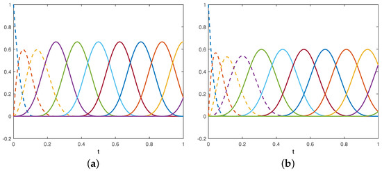
Figure 1.
Panel (a): The cubic optimal basis for . Panel (b): The quartic optimal basis for . The left edge functions are plotted as dashed lines.
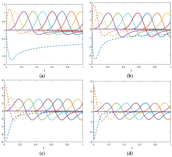
Figure 2.
The fractional derivative of the cubic optimal basis. The left edge functions are plotted as dashed lines. Panel (a): . Panel (b): . Panel (c): . Panel (d): .
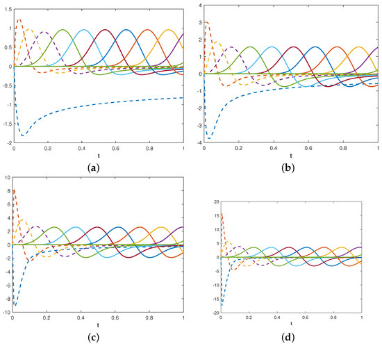
Figure 3.
The fractional derivative of the quartic optimal basis. The left edge functions are plotted as dashed lines. Panel (a): . Panel (b): . Panel (c): . Panel (d): .
For the sake of simplicity, in the tests, we set and choose equidistant nodes as collocation nodes, with . We obtain an overdetermined nonlinear system that we solved with the nonlinear least squares method. The accuracy of the numerical solution is evaluated by computing the infinity norm of the error evaluated on a refined grid:
4.1. Example 1
The aim of this example is to check the accuracy of the proposed method. To this end, we solve the nonlinear differential problem
whose exact solution is .
In the first test, we set so that the exact solution is a polynomial of degree 2. Due to the polynomial reproduction property (7), the approximation error vanishes when . In this test, we choose so that the final overdetermined nonlinear system has unknowns and equations. In Table 1 and Table 2, we list the infinity norm of the error for decreasing values of h when using the quasi-interpolant operator (13) with and . Since both approximations e reproduce quadratic polynomials, the error is very small; in particular, when , the error is in the order of the machine precision. We notice that the error increases slightly when h increases. This is due to the numerical instabilities arising when the dimensions of the nonlinear system increase. To give an idea of the stability of the nonlinear system, in Table 1 and Table 2, we also list the condition number of the Jacobian matrix.

Table 1.
The infinity norm of the error and the condition number of the Jacobian of the nonlinear system for .
Table 2.
The infinity norm of the error and the condition number of the Jacobian of the nonlinear system for .
In the second test, we check the theoretical convergence order. To this end, we solve the differential problem (17) when .
Since is an approximating operator in the spline space, the convergence of the collocation method applied to the differential problem (17) is guarantee with convergence order at least if y is sufficiently smooth [29]. As a consequence,
In Figure 4, we show the semi-log plot of the infinity norm of the error for decreasing values of when using as approximating function the quasi-interpolant operator (13) with (red line) and (blue line). The plots show that, as expected, the error decreases when h decreases. Moreover, the slope of the red and blue lines in the semi-log plots are the same as the theoretical slope . We observe that the accuracy of the approximation obtained with the optimal basis of degree is higher than the accuracy obtained for . This is due to the higher smoothness of the approximating function.
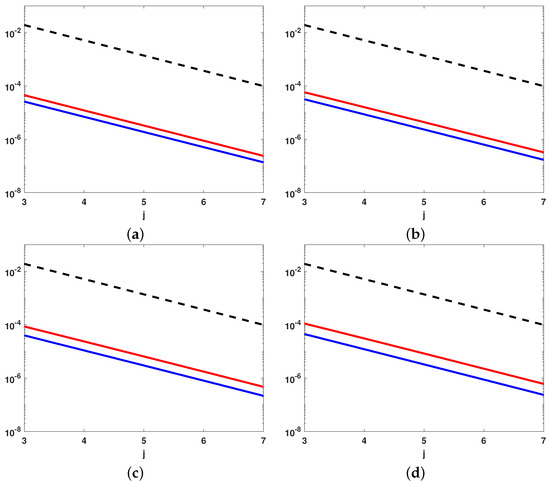
Figure 4.
The semi-log plots of the infinity norm of the error for (red line) and (blue line) when , and . The black dashed line is an arbitrary line with slope . Panel (a): . Panel (b): . Panel (c): . Panel (d): .
4.2. Example 2
In this section, we use the proposed method to solve two nonlinear differential problems arising in real-world phenomena. First of all, we consider the fractional order logistic equation
which is a nonlinear equation used to model population growth in biology and social studies. The existence and uniqueness of the solution to the logistic Equation (18) were proved in [37]. Its analytical solution is:
where is the Mittag–Leffler function:
(cf. [38]). In Figure 5, we show the numerical solutions and and the errors and for different values of when , and .
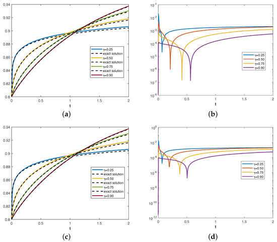
Figure 5.
Panel (a): The numerical solution (colored lines) and the exact solution (dashed black lines) for different values of . Panel (b): The error for different values of . Panel (c): The numerical solution (colored lines) and the exact solution (dashed black lines) for different values of . Panel (d): The error for different values of .
In the second example, we solve a nonlinear multiterm fractional differential equation, i.e., a differential equation characterized by the presence of both ordinary and fractional derivatives. This kind of equations is used to model viscoelastic materials. In particular, we consider the differential equation
whose exact solution is . In Figure 6, we show the numerical solutions and and the errors and for different values of when .

Figure 6.
Panel (a): The numerical solution (colored lines) and the exact solution (dashed black lines) for different values of . Panel (b): The error for different values of . Panel (c): The numerical solution (colored lines) and the exact solution (dashed black lines) for different values of . Panel (d): The error for different values of .
The plots in Figure 5 and Figure 6 show that the approximate solution has a good accuracy even in case of low values of . The accuracy increases as the order of the fractional derivative increases because the smoothness of the known term of the differential equation increases. Finally, we notice that, due to the interpolation property of the optimal basis, the error in the initial point is very small.
5. Conclusions
We presented a collocation method based on spline quasi-interpolant operators suitable to solve nonlinear differential problems having fractional derivative in time. The numerical results in Section 4 show that the method is convergent and accurate. We notice that the polynomial reproduction property (7) is a key ingredient to obtain high accuracy. Moreover, the approximations obtained by the quasi-interpolant operator (13) have shape-preserving properties. This means that the approximating function preserves the shape of the function to be approximated. This can be useful in applications where we need to preserve the sign or the monotonicity of the approximation.
Some issues are worth analyzing in detail. First, in this paper, we used equidistant collocation nodes. It is well known that different distributions of nodes could improve the accuracy of spline collocation methods [11,14]. The behavior of the present method when using other kinds of nodes, such as Gaussian points or graded meshes, should be analyzed. Secondly, the stability and convergence of the method and the behavior of the conditioning of the nonlinear system should be studied in detail. Some preliminary results in the case when can be found in [36]. A thorough analysis of the general case is under study. Finally, we observe that the method can be easily extended to other kinds of fractional differential equations, such as boundary value problems (see [39]). This will be the subject of a forthcoming paper.
Author Contributions
E.P. and F.P. contributed equally to the manuscript. All authors have read and agreed to the published version of the manuscript.
Funding
This research was partially funded by Gruppo Nazionale per il Calcolo Scientifico (Istituto Nazionale di Alta Matematica ‘Francesco Severi’), grant INdAM–GNCS Project 2020 “Costruzione di metodi numerico/statistici basati su tecniche multiscala per il trattamento di segnali e immagini ad alta dimensionalità”.
Data Availability Statement
Data is contained within the article.
Conflicts of Interest
The authors declare no conflict of interest.
References
- Kilbas, A.A.; Srivastava, H.M.; Trujillo, J.J. Theory and Applications of Fractional Differential Equations; Elsevier Science (North-Holland): Amsterdam, The Netherlands, 2006. [Google Scholar]
- Hilfer, R. Applications of Fractional Calculus in Physics; World Scientific: Singapore, 2000. [Google Scholar]
- Mainardi, F. Fractional Calculus and Waves in Linear Viscoelasticity: An Introduction to Mathematical Models; World Scientific: Singapore, 2010. [Google Scholar]
- Baleanu, D.; Diethelm, K.; Scalas, E.; Trujillo, J.J. Fractional Calculus: Models and Numerical Methods; World Scientific: Singapore, 2016. [Google Scholar]
- Li, C.; Zeng, F. Numerical Methods for Fractional Calculus; CRC Press: Boca Raton, FL, USA, 2015; Volume 24. [Google Scholar]
- Zayernouri, M.; Karniadakis, G.E. Fractional spectral collocation method. SIAM J. Sci. Comput. 2014, 36, A40–A62. [Google Scholar] [CrossRef]
- Zhang, Z.; Zeng, F.; Karniadakis, G.E. Optimal error estimates of spectral Petrov–Galerkin and collocation methods for initial value problems of fractional differential equations. SIAM J. Numer. Anal. 2015, 53, 2074–2096. [Google Scholar] [CrossRef]
- Doha, E.H.; Bhrawy, A.H.; Ezz-Eldien, S.S. A Chebyshev spectral method based on operational matrix for initial and boundary value problems of fractional order. Comput. Math. Appl. 2011, 62, 2364–2373. [Google Scholar] [CrossRef]
- Khader, M.; El Danaf, T.; Hendy, A. Efficient spectral collocation method for solving multi-term fractional differential equations based on the generalized Laguerre polynomials. Fract. Calc. Appl. 2012, 3, 1–14. [Google Scholar]
- Russell, R.; Shampine, L.F. A collocation method for boundary value problems. Numer. Math. 1972, 19, 1–28. [Google Scholar] [CrossRef]
- de Boor, C.; Swartz, B. Collocation at Gaussian points. SIAM J. Numer. Anal. 1973, 10, 582–606. [Google Scholar] [CrossRef]
- Ascher, U. Discrete least squares approximations for ordinary differential equations. SIAM J. Numer. Anal. 1978, 15, 478–496. [Google Scholar] [CrossRef]
- Blank, L. Numerical Treatment of Differential Equations of Fractional Order; Numerical Analysis Report; Department of Mathematics, University of Manchester: Manchester, UK, 1996. [Google Scholar]
- Pedas, A.; Tamme, E. On the convergence of spline collocation methods for solving fractional differential equations. J. Comput. Appl. Math. 2011, 235, 3502–3514. [Google Scholar] [CrossRef]
- Pedas, A.; Tamme, E. Numerical solution of nonlinear fractional differential equations by spline collocation methods. J. Comput. Appl. Math. 2014, 255, 216–230. [Google Scholar] [CrossRef]
- Kolk, M.; Pedas, A.; Tamme, E. Smoothing transformation and spline collocation for linear fractional boundary value problems. Appl. Math. Comput. 2016, 283, 234–250. [Google Scholar] [CrossRef]
- Pezza, L.; Pitolli, F. A fractional spline collocation-Galerkin method for the time-fractional diffusion equation. Commun. Appl. Ind. Math. 2018, 9, 104–120. [Google Scholar] [CrossRef]
- Pitolli, F. A collocation method for the numerical solution of nonlinear fractional dynamical systems. Algorithms 2019, 12, 156. [Google Scholar] [CrossRef]
- Pitolli, F.; Pezza, L. A fractional spline collocation method for the fractional-order logistic equation. In Approximation Theory XV: San Antonio 2016; Fasshauer, G.E., Schumaker, L.L., Eds.; Springer Proceedings in Mathematics & Statistics 201; Springer: Berlin/Heidelberg, Germany, 2017; pp. 307–318. [Google Scholar]
- Mazza, M.; Donatelli, M.; Manni, C.; Speleers, H. On the matrices in B-spline collocation methods for Riesz fractional equations and their spectral properties. arXiv 2021, arXiv:2106.14834. [Google Scholar]
- Rabinowitz, P. Application of approximating splines for the solution of Cauchy singular integral equations. Appl. Numer. Math. 1994, 15, 285–297. [Google Scholar] [CrossRef]
- de Boor, C.; Fix, G. Spline approximations by quasi-interpolants. J. Approx. Theory 1973, 8, 19–45. [Google Scholar] [CrossRef]
- Caliò, F.; Marchetti, E.; Rabinowitz, P. On the numerical solution of the generalized Prandtl equation using variation-diminishing splines. J. Comput. Appl. Math. 1995, 60, 297–307. [Google Scholar] [CrossRef]
- Gori, L.; Santi, E.; Cimoroni, M. Projector-splines in the numerical solution of inetgro-differential equations. Comput. Math. Appl. 1998, 35, 107–116. [Google Scholar] [CrossRef]
- Foucher, F.; Sablonnière, P. Quadratic spline quasi-interpolants and collocation methods. Math. Comput. Simul. 2009, 79, 3455–3465. [Google Scholar] [CrossRef][Green Version]
- Pellegrino, E.; Pezza, L.; Pitolli, F. Quasi-interpolant operators and the solution of fractional differential problems. In Approximation Theory XVI. Nashville 2019; Fasshauer, G.E., Neamtu, M., Schumaker, L.L., Eds.; Springer: Berlin/Heidelberg, Germany, 2020. [Google Scholar]
- Pellegrino, E.; Pezza, L.; Pitolli, F. A collocation method based on discrete spline quasi-interpolatory operators for the solution of time fractional differential equations. Fractal Fract. 2021, 5, 5. [Google Scholar] [CrossRef]
- Diethelm, K. The Analysis of Fractional Differential Equations: An Application-Oriented Exposition Using Differential Operators of Caputo Type; Springer Science & Business Media: Berlin/Heidelberg, Germany, 2010. [Google Scholar]
- de Boor, C. A Practical Guide to Splines; Springer: Berlin/Heidelberg, Germany, 1978. [Google Scholar]
- Schumaker, L. Spline Functions: Basic Theory; Cambridge University Press: Cambridge, UK, 2007. [Google Scholar]
- Pitolli, F. Optimal B-spline bases for the numerical solution of fractional differential problems. Axioms 2018, 7, 46. [Google Scholar] [CrossRef]
- Carnicer, J.M.; Peña, J.M. Totally positive bases for shape preserving curve design and optimality of B-splines. Comput. Aided Geom. Design 1994, 11, 633–654. [Google Scholar] [CrossRef]
- Goodman, T. Shape preserving representations. In Mathematical Methods in Computer Aided Geometric Design; Lyche, T., Schumaker, L.L., Eds.; Academic Press: Cambridge, MA, USA, 1989; pp. 333–351. [Google Scholar]
- Lyche, T.; Schumaker, L.L. Local spline approximation methods. J. Approx. Theory 1975, 15, 294–325. [Google Scholar] [CrossRef]
- Sablonnière, P. Recent progress on univariate and multivariate polynomial and spline quasi-interpolants. In Trends and Applications in Constructive Approximation; De Bruin, M., Mache, D., Szabados, J., Eds.; ISNM; Birkhäuser Verlag: Basel, Switzerland, 2005; Volume 177, pp. 229–245. [Google Scholar]
- Pellegrino, E.; Pezza, L.; Pitolli, F. A collocation method in spline spaces for the solution of linear fractional dynamical systems. Math. Comput. Simul. 2020, 176, 266–278. [Google Scholar] [CrossRef]
- El-Sayed, A.; El-Mesiry, A.; El-Saka, H. On the fractional-order logistic equation. Appl. Math. Lett. 2007, 20, 817–823. [Google Scholar] [CrossRef]
- West, B.J. Exact solution to fractional logistic equation. Phys. A Stat. Mech. Its Appl. 2015, 429, 103–108. [Google Scholar] [CrossRef]
- Pitolli, F. On the numerical solution of fractional boundary value problems by a spline quasi-interpolant operator. Axioms 2020, 9, 61. [Google Scholar] [CrossRef]
Publisher’s Note: MDPI stays neutral with regard to jurisdictional claims in published maps and institutional affiliations. |
© 2021 by the authors. Licensee MDPI, Basel, Switzerland. This article is an open access article distributed under the terms and conditions of the Creative Commons Attribution (CC BY) license (https://creativecommons.org/licenses/by/4.0/).