Accelerated Modified Tseng’s Extragradient Method for Solving Variational Inequality Problems in Hilbert Spaces

Abstract

The aim of this paper is to propose a new iterative algorithm to approximate the solution for a variational inequality problem in real Hilbert spaces. A strong convergence result for the above problem is established under certain mild conditions. Our proposed method requires the computation of only one projection onto the feasible set in each iteration. Some numerical examples are presented to support that our proposed method performs better than some known comparable methods for solving variational inequality problems.

1. Introduction

Suppose C is a nonempty closed convex subset of a real Hilbert space H with the inner product $\langle .,.\rangle$ which induces the norm $\parallel .\parallel$, and A is a self mapping on H. The variational inequality problem (VIP) for an operator A on $C\subset H$ is to find a point $x^{\ast }\in C$ such that the following is the case.

$$\langle A{x}^{\ast },x-x^{\ast }\rangle \ge 0\mathit{for}\mathrm{each}x\in C.$$

(1)

In this paper, we denote the solution set of (VIP) (1) by $\Gamma .$

The theory of variational inequalities problems (VIP) was introduced by Stampacchia [1]. It has been proved that the (VIP) problem arise from various mathematical models connected with real life problems. Over the years, VIP has attracted the attention of well-known mathematicians due to its applications in several fields of interest such as sciences and engineering. Interest in (VIP) stems from the fact that it is applicable in solving several real life problems that are of physical interest, such as the problem of the steady filtration of a liquid through a porous membrane in several dimensions, the problem of lubrication, the motion of a fluid past a certain profile and the small deflections of an elastic beam (See, e.g., [2]).

The optimization problem comprises maximizing or minimizing some function f relative to some set $S.$ The function f provides room for the comparison of different options relative to determining which is the best. We write the optimization problem as follows:

$$optimiz{e}_{x\in S}f\left(x\right)$$

where $optimize$ stands for min or max, and $f:{\mathbb{R}}^n\to \mathbb{R}$ denotes the objective function. We note that the optimal solution of a maximization problem of the following:

$$\underset{x\in S}{max}f\left(x\right)$$

coincide with the optimal solutions of the minimization problem:

$$\underset{x\in S}{min}-f\left(x\right)$$

and we have ${max}_{x\in S}f\left(x\right)=-{min}_{x\in S}(-f\left(x\right)).$

The two popular methods of solving (VIP) (1) are the projection method and the regularized method. Several authors have developed efficient iterative algorithms for solving the (VIP) (1). The projection-type methods are well developed in the literature (see, for example, [3,4,5,6,7]). The well-known projected gradient algorithm method, which is useful in solving the minimization problem $f\left(x\right)$ subject to $x\in C$ is given as follows:

$$x_{n+1}=P_C(x_n-{\alpha }_n▽f\left(x_n\right)),n\ge 0,$$

(2)

where the real sequence $\left\{{\alpha }_n\right\}$ of parameters satisfies some conditions, $P_C$ is the well-known metric projection of vectors in H onto C and $▽f$ denotes the gradient of $f.$ Interested readers may refer to [8] for convergence analysis of the above method for the case when $f:H\to \mathbb{R}$ is convex and differentiable. The method (2) was extended to the (VIP) (1) problem by replacing the gradient of f with the operator A and by generating a sequence $\left\{x_n\right\}$ as follows.

$$x_{n+1}=P_C(x_n-{\alpha }_{n}A{x}_n),n\ge 0.$$

(3)

Note that the major disadvantage of this method is the restriction that the operator A is strongly monotone or inverse strongly monotone ([9]) for the convergence of this method. In 1976, Korpelevich [10] removed this strong condition by introducing the extragradient method for solving saddle point problems. This well-known method was extended to solving variational inequality problems (VIP) in both Hilbert and Euclidean spaces (see [10,11]). For the onvergence of this method, the only restriction on the operator A is monotonocity and L-Lipschitz continuity. The extragradient method is given as follows:

$$\left\{\begin{array}{ccc}{y}_n=P_C(x_n-\lambda A{x}_n)\hfill & \hfill & \\ x_{n+1}=P_C(x_n-\lambda A{y}_n),\hfill & \hfill \end{array}\right.$$

(4)

where $\lambda \in (0,\frac{1}{L}).$ If the solution set $\Gamma$ of the (VIP) is nonempty, then the sequence $\left\{x_n\right\}$ generated by the iterative method (4) converges weakly to an element in $\Gamma .$

Clearly, by using the above method, one needs to compute two projections onto the set C in every iteration. It is well known that the projection onto a closed convex set $C\subset H$ has a close relationship with the minimum distance problem, which may require a restrictive amount of computation time. To solve this problem, Censor et al. [4] introduced the subgradient extragradient method by modifying iterative algorithm (4). They replaced the two projections in the extragradient method (4) onto the set C with one projection onto the set $C\subset H$ and one projection onto a half-space, which is easier to calculate.

The Censor et al. [4] subgradient extragradient method is given as follows:

$$\left\{\begin{array}{ccc}{y}_n=P_C(x_n-\lambda A{x}_n)\hfill & \hfill & \\ T_n=\{x\in H:\langle x_n-\lambda A{x}_n-y_n,x-y_n\rangle \le 0\}\hfill & \hfill & \\ x_{n+1}=P_{T_n}(x_n-\lambda A{y}_n),\hfill & \hfill \end{array}\right.$$

(5)

where $\lambda \in (0,\frac{1}{L}).$ Several authors have studied the subgradient extragradient method and proved some useful and applicable results (see, for example, [7,12] and the references therein).

In 2000, Tseng [13] developed a method involving only one projection for solving the variational inequality problem (VIP) (1). The Tseng’s extragradient method is as follows:

$$\left\{\begin{array}{ccc}{y}_n=P_C(x_n-\lambda A{x}_n)\hfill & \hfill & \\ x_{n+1}=y_n-\lambda (A{y}_n-A{x}_n),\hfill & \hfill \end{array}\right.$$

(6)

where $\lambda \in (0,\frac{1}{L}).$ Recently, many well-known mathematicians developed some modified Tseng’s extragradient methods for solving variational inequality problems (VIP) (see, e.g., [14,15,16] and the references therein).

The inertial-type iterative methods are based on a discrete version of a second order dissipative dynamical system (see [7,17,18]). These methods can be seen as a process meant to accelerate the rate of convergence of a given method (see, e.g., [19,20,21]). In 2001, Alvarez and Attouch [19] applied the inertial method to derive a proximal algorithm for solving the problem of finding zero of a maximal monotone operator. Their method is given as follows.

Given $x_{n-1},x_n\in H$ and two parameters ${\theta }_n\in [0,1),$ ${\lambda }_n>0,$ $x_{n+1}\in H$ is obtained such that the following is the case:

$$0\in {\lambda }_{n}A\left(x_{n+1}\right)+x_{n+1}-x_n-{\theta }_n(x_n-x_{n-1}).$$

(7)

The above method can be written equivalently as follows:

$$x_{n+1}=J_{{\lambda }_n}^A(x_n+{\theta }_n(x_n-x_{n-1}),$$

(8)

where $J_{{\lambda }_n}^A$ is the resolvent of the operator A with the given parameter ${\lambda }_n$, and the inertial is induced by the term ${\theta }_n(x_n-x_{n-1}).$

Several algorithms with faster convergence rate via the use of inertial methods have appeared in literature recently (see, e.g., [22,23]). These algorithms include inertial forward-backward splitting methods ([24]), the inertial Douglas–Rachford splitting method ([25]), inertial ADMM ([26]), inertial proximal-extragradient method ([27]), inertial contraction method ([28]) and inertial forward-backward-forward method ([29]), among others.

Motivated by the results above, we propose a new algorithm for solving variational inequality problems in real Hilbert spaces. Our proposed method combines the modified Tseng’s extragradient method [13], the viscosity method [30] and the Picard–Mann method [31]. Our method requires the computation of only one projection onto the feasible set (solution set) in each iteration. We establish a strong convergence theorem of the proposed algorithm under certain mild conditions. Furthermore, with the help of several numerical illustrations, we show that the proposed method performs better than some known methods for solving variational inequality problems.

This paper is organized as follows: In Section 2, some preliminary definitions and known results that are needed in this study are given. In Section 3, a modified Tseng’s extragradient algorithm is proposed, and a strong convergence theorem for the method is presented. In Section 4, some numerical illustrations are given to show that method presented herein performs better than some existing methods. Section 5 contains the concluding remarks of this paper.

2. Preliminaries

Let H be a real Hilbert space, we recall the following definitions.

Definition 1.

A mapping$A:H\to H$is said to be:

(i)

L-Lipschitz continuous with$L>0$if the following is the case.

$$\parallel Ax-Ay\parallel \le L\parallel x-y\parallel \mathit{for}\mathit{all}x,y\in H.$$

(9)

If$L\in [0,1)$then A is called a contraction mapping. If$L=1,$then A is called nonexpansive mapping.

(ii)

It is monotone if the following is the case.

$$\langle Ax-Ay,x-y\rangle \ge 0,\mathit{for}\mathit{all}x,y\in H.$$

(10)

(iii)

A is called strictly monotone if for any$x\ne y$, the following is the case:

$$\langle x-y,A\left(x\right)-A\left(y\right)\rangle >0$$

and the equality is possible only if$x=y.$

(iv)

A is called strongly monotone if for any$x,y\in H$, the following is the case:

$$\langle x-y,A\left(x\right)-A\left(y\right)\rangle \ge \alpha (\parallel x-y\parallel )\parallel x-y\parallel$$

where the nonnegative function$\alpha \left(t\right)$defined at$t\ge 0$satisfies the condition$\alpha \left(0\right)=0$and$\alpha \left(t\right)\to \infty$when$t\to \infty .$

(v)

A is called pseudomonotone if the following is the case.

$$\langle A\left(y\right),x-y\rangle \ge 0\Rightarrow \langle A\left(x\right),x-y\rangle \ge 0,\forall x,y\in H.$$

For every $x\in H,$ there exists a unique point $P_{C}x$ in $C\subset H$ such that the following is the case:

$$\parallel x-P_{C}x\parallel \le \parallel x-y\parallel$$

(11)

for each $y\in C$ (see, e.g., [32]). A mapping $P_C$ is known as the metric projection of H onto $C\subset H.$ It is known that the mapping $P_C$ is nonexpansive.

Next, we recall the following lemmas which will be useful in this paper.

Lemma 1

([32]). Given that C is a closed convex subset of a real Hilbert space H and $x\in H$, we have the following:

(i)

$\parallel P_{C}x-P_C{y\parallel }^2\le \langle P_{C}x-P_{C}y,x-y\rangle$ for all $y\in H$;

(ii)

$\parallel P_C{x-y\parallel }^2\le {\parallel x-y\parallel }^2-{\parallel x-P_{C}x\parallel }^2$ for all $y\in H$;

(iii)

$$z=P_{C}x\mathit{if}\mathit{and}\mathit{only}\mathit{if}\langle x-z,z-y\rangle \ge 0$$

for all $y\in C.$

For more properties of the metric projection $P_C,$ the interested reader may refer to Section 3 of [32].

Let $A:H\to H$. The fixed point problem $\left(FP\right)$ is formulated as follows.

$$\mathrm{find}x\in H\mathrm{such}\mathrm{that}x=A\left(x\right).$$

(12)

The set of fixed point of the operator A is denoted by $F\left(A\right)$, and we assume that $F\left(A\right)\ne \varnothing .$ Our interest in this paper is to find a point $x\in H$ such that the following is the case.

$$x\in \Gamma \cap F\left(A\right).$$

(13)

The weak convergence of the sequence $\left\{x_n\right\}$ to x is denoted by $x_n\rightharpoonup x$ as $n\to \infty ,$ and we denote the strong convergence of $\left\{x_n\right\}$ to x by $x_n\to x$ as $n\to \infty .$

For each $x,y\in H$ and $\alpha \in \mathbb{R},$ we recall the following inequalities in Hilbert spaces.

$${\parallel \alpha x+(1-\alpha )y\parallel }^2={\alpha \parallel x\parallel }^2+{(1-\alpha )\parallel y\parallel }^2-\alpha (1-\alpha ){\parallel x-y\parallel }^2.$$

(14)

$${\parallel x+y\parallel }^2\le {\parallel x\parallel }^2+2\langle y,x+y\rangle .$$

(15)

$${\parallel x+y\parallel }^2={\parallel x\parallel }^2+2\langle x,y\rangle +{\parallel y\parallel }^2.$$

(16)

The following lemmas will be needed in this paper.

Lemma 2

([33,34]). Let $\left\{a_n\right\}$ be a sequence of nonnegative real numbers, $\left\{{\alpha }_n\right\}$ denotes a sequence of real numbers in $(0,1)$ with ${\sum }_{n=1}^{\infty }{\alpha }_n=\infty$ and $\left\{b_n\right\}$ denotes a sequence of real numbers. We will assume that the following is the case.

$$a_{n+1}\le (1-{\alpha }_n)a_n+{\alpha }_n{b}_n,\forall n\ge 1.$$

If ${lim\; sup}_{k\to \infty }{b}_{n_k}\le 0$ for every subsequence $\left\{a_{n_k}\right\}$ of $\left\{a_n\right\}$ satisfying ${lim\; inf}_{k\to \infty }(a_{n_{k+1}}-a_{n_k})\ge 0,$ then ${lim}_{n\to \infty }{a}_n=0.$

3. Main Results

We assume that the following condition is satisfied.

Condition 1.

The feasible set C is a non-empty, closed and convex subset of the real Hilbert space $H.$ The mapping $A:H\to H$ is monotone and L-Lipschitz continuous on $H,$ with the solution set of (VIP) (1); $\Gamma \ne \varnothing$ and $f:H\to H$ is a contraction mapping with the contraction parameter $k\in [0,1).$

We now propose the following algorithm.

• Step 0: Given $\left\{{\alpha }_n\right\}\subset [0,\alpha )$ for some $\alpha >0,$$\lambda \in (0,\frac{1}{L}),$$\left\{{\theta }_n\right\}\subset (a,b)\subset (0,1-{\beta }_n)$ and $\left\{{\beta }_n\right\}\subset (0,1)$ satisfying the following conditions:

  $$\underset{n\to \infty }{lim}{\beta }_n=0,\sum _{n=1}^{\infty }{\beta }_n=\infty .$$

  (17)

  choose the initial $x_0,x_1\in C$ and set $n:=1.$
• Step 1: Set the following:

  $$w_n=x_n+{\alpha }_n(x_n-x_{n-1}),$$

  (18)

  and compute the following.

  $$y_n=P_C(w_n-\lambda A{w}_n).$$

  (19)
  If $y_n=w_n,$ then stop the computation. $y_n$ is a solution to the problem (VIP). Otherwise, proceed to Step 2.
• Step 2: Set the following:

  $$h_n=(1-{\theta }_n-{\beta }_n)f\left(x_n\right)+{\theta }_n{z}_n$$

  (20)

  and compute the following:

  $$x_{n+1}=f\left(h_n\right),$$

  (21)

  where

  $$z_n=y_n-\lambda (A{y}_n-A{w}_n).$$

  (22)

  Set $n:=n+1$ and proceed to Step 1.

Next, we prove the following results.

Theorem 1.

Suppose Condition 1 holds and the following is the case.

$$\underset{n\to \infty }{lim}\frac{{\alpha }_n}{{\beta }_n}\parallel x_n-x_{n-1}\parallel =0.$$

(23)

The sequence $\left\{x_n\right\}$ generated by the algorithm converges strongly to an element $p\in \Gamma ,$ such that $p=P_{\Gamma }\circ f\left(p\right).$

Proof. 

Claim I: We claim that the sequence $\left\{x_n\right\}$ is bounded for each $p=P_{VI(C,A)\circ f\left(p\right)}.$ We begin by proving the following.

$$\parallel z_n{-p\parallel }^2\le \parallel w_n{-p\parallel }^2-(1-{\lambda }^2{L}^2){\parallel y_n-w_n\parallel }^2.$$

(24)

Using (22) together with (10), (11), (19) and Lemma 1 (ii), we have the following.

$$\begin{array}{ccc}\parallel z_n{-p\parallel }^2\hfill & =\hfill & \parallel y_n-\lambda (A{y}_n-A{w}_n){-p\parallel }^2\hfill \\ & =\hfill & \parallel y_n{-p\parallel }^2+{\lambda }^2{\parallel A{y}_n-A{w}_n\parallel }^2-2\lambda \langle y_n-p,A{y}_n-A{w}_n\rangle \hfill \\ & =\hfill & \parallel P_C(w_n-\lambda A{w}_n){-p\parallel }^2+{\lambda }^2{\parallel A{y}_n-A{w}_n\parallel }^2-2\lambda \langle y_n-p,A{y}_n-A{w}_n\rangle \hfill \\ & \le \hfill & \parallel w_n-\lambda A{w}_n{-p\parallel }^2-\parallel w_n-\lambda A{w}_n-P_C(w_n-\lambda A{w}_n){\parallel }^2+{\lambda }^2{\parallel A{y}_n-A{w}_n\parallel }^2-\hfill \\ & \hfill & 2\lambda \langle y_n-p,A{y}_n-A{w}_n\rangle \hfill \\ & =\hfill & \parallel w_n-\lambda A{w}_n{-p\parallel }^2-\parallel w_n-\lambda A{w}_n-y_n{\parallel }^2+{\lambda }^2{\parallel A{y}_n-A{w}_n\parallel }^2-\hfill \\ & \hfill & 2\lambda \langle y_n-p,A{y}_n-A{w}_n\rangle \hfill \\ & \le \hfill & \parallel w_n{-p\parallel }^2-2\lambda \langle A{w}_n,w_n-p-\lambda A{w}_n\rangle -{\parallel w_n-y_n\parallel }^2+2\lambda \langle A{w}_n,w_n-y_n-\lambda A{w}_n\rangle \hfill \\ & \hfill & +{\lambda }^2{\parallel A{y}_n-A{w}_n\parallel }^2-2\lambda \langle y_n-p,A{y}_n-A{w}_n\rangle \hfill \\ & =\hfill & \parallel w_n{-p\parallel }^2-2\lambda \langle A{y}_n,y_n-p\rangle -\parallel w_n-y_n{\parallel }^2+{\lambda }^2{\parallel A{y}_n-A{w}_n\parallel }^2\hfill \\ & =\hfill & \parallel w_n{-p\parallel }^2-2\lambda \langle A{y}_n-Ap,y_n-p\rangle -2\lambda \langle Ap,y_n-p\rangle -{\parallel w_n-y_n\parallel }^2+\hfill \\ & \hfill & {\lambda }^2{\parallel A{y}_n-A{w}_n\parallel }^2.\hfill \end{array}$$

(25)

Using the fact that the mapping A is monotone and L-Lipschitz continuous, we have the following from inequality (25).

$$\begin{array}{ccc}\parallel z_n{-p\parallel }^2\hfill & \le \hfill & \parallel w_n{-p\parallel }^2-\parallel w_n-y_n{\parallel }^2+{\lambda }^2{\parallel A{y}_n-A{w}_n\parallel }^2\hfill \\ & \le \hfill & \parallel w_n{-p\parallel }^2-\parallel w_n-y_n{\parallel }^2+{\lambda }^2{L}^2{\parallel y_n-w_n\parallel }^2\hfill \\ & =\hfill & \parallel w_n{-p\parallel }^2-(1-{\lambda }^2{L}^2){\parallel y_n-w_n\parallel }^2.\hfill \end{array}$$

(26)

This implies the following.

$$\parallel z_n-p\parallel \le \parallel w_n-p\parallel .$$

(27)

By (18), we have the following estimate.

$$\begin{array}{ccc}\parallel w_n-p\parallel \hfill & =\hfill & \parallel x_n+{\alpha }_n(x_n-x_{n-1})-p\parallel \hfill \\ & \le \hfill & \parallel x_n-p\parallel +{\alpha }_n\parallel x_n-x_{n-1}\parallel \hfill \\ & =\hfill & \parallel x_n-p\parallel +{\beta }_n.\frac{{\alpha }_n}{{\beta }_n}\parallel x_n-x_{n-1}\parallel .\hfill \end{array}$$

(28)

Using the condition that $\frac{{\alpha }_n}{{\beta }_n}\parallel x_n-x_{n-1}\parallel \to 0$ in (23), it follows that there exists a constant ${\ell }_1>0$ such that the following is the case.

$$\frac{{\alpha }_n}{{\beta }_n}\parallel x_n-x_{n-1}\parallel \le {\ell }_1,\forall n\ge 1.$$

(29)

Using (28) and (29) in (27), we have the following.

$$\parallel z_n-p\parallel \le \parallel w_n-p\parallel \le \parallel x_n-p\parallel +{\beta }_n{\ell }_1.$$

(30)

Using (21) and the condition that f is a contraction mapping, we have the following.

$$\begin{array}{ccc}\parallel x_{n+1}-p\parallel \hfill & =\hfill & \parallel f\left(h_n\right)-p\parallel \hfill \\ & =\hfill & \parallel f\left(h_n\right)-f\left(p\right)+f\left(p\right)-p\parallel \hfill \\ & \le \hfill & \parallel f\left(h_n\right)-f\left(p\right)\parallel +\parallel f\left(p\right)-p\parallel \hfill \\ & \le \hfill & k\parallel h_n-p\parallel +\parallel f\left(p\right)-p\parallel .\hfill \end{array}$$

(31)

Next, by using (20) together with (30), we have the following:

$$\begin{array}{ccc}\parallel h_n-p\parallel \hfill & =\hfill & \parallel (1-{\theta }_n-{\beta }_n)f\left(x_n\right)+{\theta }_n{z}_n-p\parallel \hfill \\ & =\hfill & \parallel (1-{\theta }_n-{\beta }_n)(f\left(x_n\right)-p)+{\theta }_n(z_n-p)-{\beta }_{n}p\parallel \hfill \\ & \le \hfill & \parallel (1-{\theta }_n-{\beta }_n)(f\left(x_n\right)-p)+{\theta }_n(z_n-p)\parallel +{\beta }_n\parallel p\parallel \hfill \\ & \le \hfill & (1-{\theta }_n-{\beta }_n)\parallel f\left(x_n\right)-p\parallel +{\theta }_n\parallel z_n-p\parallel +{\beta }_n\parallel p\parallel \hfill \\ & \le \hfill & (1-{\theta }_n-{\beta }_n)\parallel f\left(x_n\right)-f\left(p\right)\parallel +(1-{\theta }_n-{\beta }_n)\parallel f\left(p\right)-p\parallel +{\theta }_n\parallel z_n-p\parallel +{\beta }_n\parallel p\parallel \hfill \\ & \le \hfill & k(1-{\theta }_n-{\beta }_n)\parallel x_n-p\parallel +(1-{\theta }_n-{\beta }_n)\parallel f\left(p\right)-p\parallel +{\theta }_n\parallel z_n-p\parallel +{\beta }_n\parallel p\parallel \hfill \\ & \le \hfill & (1-{\theta }_n-{\beta }_n)\parallel x_n-p\parallel +(1-{\theta }_n-{\beta }_n)\parallel f\left(p\right)-p\parallel +{\theta }_n[\parallel x_n-p\parallel +{\beta }_n{\ell }_1]+{\beta }_n\parallel p\parallel \hfill \\ & =\hfill & (1-{\beta }_n)\parallel x_n-p\parallel +(1-{\theta }_n-{\beta }_n)\parallel f\left(p\right)-p\parallel +{\beta }_n({\theta }_n{\ell }_1+\parallel p\parallel )\hfill \\ & \le \hfill & (1-{\beta }_n)\parallel x_n-p\parallel +(1-{\theta }_n-{\beta }_n)\parallel f\left(p\right)-p\parallel +{\beta }_n{\ell }_2,\hfill \end{array}$$

(32)

for some ${\ell }_2>0.$

Using (32) in (31), we have the following:

$$\begin{array}{ccc}\parallel x_{n+1}-p\parallel \hfill & \le \hfill & k(1-{\beta }_n)\parallel x_n-p\parallel +k(1-{\theta }_n-{\beta }_n)\parallel f\left(p\right)-p\parallel +{\beta }_{n}k{\ell }_2+\parallel f\left(p\right)-p\parallel \hfill \\ & \le \hfill & (1-{\beta }_n)\parallel x_n-p\parallel +(1-{\theta }_n-{\beta }_n)\parallel f\left(p\right)-p\parallel +{\beta }_{n}k{\ell }_2+\parallel f\left(p\right)-p\parallel \hfill \\ & =\hfill & (1-{\beta }_n)\parallel x_n-p\parallel +(2-{\theta }_n-{\beta }_n)\parallel f\left(p\right)-p\parallel +{\beta }_{n}k{\ell }_2\hfill \\ & \le \hfill & (1-{\beta }_n)\parallel x_n-p\parallel +(1-k)\frac{{\ell }_3+2\parallel f\left(p\right)-p\parallel }{1-k}\hfill \\ & \le \hfill & max\left\{\parallel x_n-p\parallel ,\frac{{\ell }_3+2\parallel f\left(p\right)-p\parallel }{1-k}\right\}\hfill \\ & ⋮\hfill & \\ & \le \hfill & max\left\{\parallel x_0-p\parallel ,\frac{{\ell }_3+2\parallel f\left(p\right)-p\parallel }{1-k}\right\},\hfill \end{array}$$

(33)

for some ${\ell }_3>0.$ This implies that the sequence $\left\{x_n\right\}$ is bounded. Therefore, it follows that $\left\{z_n\right\},$$\left\{h_n\right\},$$\left\{f\left(h_n\right)\right\}$ and $\left\{w_n\right\}$ are bounded.

Claim II: We have the following case:

$$(1-{\beta }_n)(1-{\lambda }^2{L}^2)\parallel y_n-w_n{\parallel }^2\le 3(1-{\beta }_n)\parallel x_n{-p\parallel }^2-{\parallel x_{n+1}-p\parallel }^2+{\beta }_n{\ell }_{10},$$

for some ${\ell }_{10}>0.$ By using (21) together with (11), we obtain the following:

$$\begin{array}{ccc}\parallel x_{n+1}{-p\parallel }^2\hfill & =\hfill & \parallel f\left(h_n\right){-p\parallel }^2\hfill \\ & =\hfill & \parallel f\left(h_n\right)-f\left(p\right)+f\left(p\right){-p\parallel }^2\hfill \\ & =\hfill & \parallel f\left(h_n\right)-f\left(p\right){\parallel }^2+{\parallel f\left(p\right)-p\parallel }^2+2\langle f\left(h_n\right)-f\left(p\right),f\left(p\right)-p\rangle \hfill \\ & \le \hfill & k^2\parallel h_n{-p\parallel }^2{+\parallel f\left(p\right)-p\parallel }^2+2\parallel f\left(h_n\right)-f\left(p\right)\parallel \parallel f\left(p\right)-p\parallel \hfill \\ & \le \hfill & k\parallel h_n{-p\parallel }^2{+\parallel f\left(p\right)-p\parallel }^2+2k\parallel h_n-p\parallel \parallel f\left(p\right)-p\parallel \hfill \\ & \le \hfill & k\parallel h_n{-p\parallel }^2+k{\ell }_4,\hfill \end{array}$$

(34)

for some ${\ell }_4>0.$ By using (20) together with (10) and (11), we obtain the following:

$$\begin{array}{ccc}\parallel h_n{-p\parallel }^2\hfill & =\hfill & \parallel (1-{\theta }_n-{\beta }_n)f\left(x_n\right)+{\theta }_n{z}_n{-p\parallel }^2\hfill \\ & =\hfill & \parallel (1-{\theta }_n-{\beta }_n)(f\left(x_n\right)-p)+{\theta }_n(z_n-p){\parallel }^2-\hfill \\ & \hfill & 2{\beta }_n\langle (1-{\theta }_n-{\beta }_n)(f\left(x_n\right)-p)+{\theta }_n(z_n-p),p\rangle +{\beta }_n^2{\parallel p\parallel }^2\hfill \\ & \le \hfill & \parallel (1-{\theta }_n-{\beta }_n)(f\left(x_n\right)-p)+{\theta }_n(z_n-p){\parallel }^2+{\beta }_n{\ell }_5\hfill \\ & \le \hfill & {(1-{\theta }_n-{\beta }_n)}^2\parallel f\left(x_n\right){-p\parallel }^2+2(1-{\theta }_n-{\beta }_n){\theta }_n\parallel f\left(x_n\right)-p\parallel \parallel z_n-p\parallel +{\theta }_n^2{\parallel z_n-p\parallel }^2\hfill \\ & \hfill & +{\beta }_n{\ell }_5\hfill \\ & \le \hfill & {(1-{\theta }_n-{\beta }_n)}^2\parallel f\left(x_n\right){-p\parallel }^2+(1-{\theta }_n-{\beta }_n){\theta }_n{\parallel f\left(x_n\right)-p\parallel }^2+\hfill \\ & \hfill & (1-{\theta }_n-{\beta }_n){\theta }_n\parallel z_n{-p\parallel }^2+{\theta }_n^2{\parallel z_n-p\parallel }^2+{\beta }_n{\ell }_5\hfill \\ & \le \hfill & (1-{\theta }_n-{\beta }_n)(1-{\beta }_n)\parallel f\left(x_n\right){-p\parallel }^2+(1-{\beta }_n){\theta }_n{\parallel z_n-p\parallel }^2+{\beta }_n{\ell }_5,\hfill \end{array}$$

(35)

for some ${\ell }_5>0.$ Next, we have the following estimate:

$$\begin{array}{ccc}\parallel f\left(x_n\right){-p\parallel }^2\hfill & =\hfill & \parallel f\left(x_n\right)-f\left(p\right)+f\left(p\right){-p\parallel }^2\hfill \\ & =\hfill & \parallel f\left(x_n\right)-f\left(p\right){\parallel }^2+{\parallel f\left(p\right)-p\parallel }^2+2\langle f\left(x_n\right)-f\left(p\right),f\left(p\right)-p\rangle \hfill \\ & \le \hfill & \parallel f\left(x_n\right)-f\left(p\right){\parallel }^2+\parallel f\left(p\right){-p\parallel }^2+2\parallel f\left(x_n\right)-f\left(p\right)\parallel \parallel f\left(p\right)-p\parallel \hfill \\ & \le \hfill & k^2\parallel x_n{-p\parallel }^2{+\parallel f\left(p\right)-p\parallel }^2+\parallel f\left(x_n\right)-f\left(p\right){\parallel }^2+{\parallel f\left(p\right)-p\parallel }^2\hfill \\ & \le \hfill & k^2\parallel x_n{-p\parallel }^2{+\parallel f\left(p\right)-p\parallel }^2+k^2\parallel x_n{-p\parallel }^2+{\parallel f\left(p\right)-p\parallel }^2\hfill \\ & \le \hfill & 2k\parallel x_n{-p\parallel }^2+2{\parallel f\left(p\right)-p\parallel }^2\hfill \\ & \le \hfill & 2k\parallel x_n{-p\parallel }^2+{\ell }_6,\hfill \end{array}$$

(36)

for some ${\ell }_6>0.$ Hence, by combining (36) and (35), we have the following:

$$\parallel h_n{-p\parallel }^2\le 2k(1-{\theta }_n-{\beta }_n)(1-{\beta }_n)\parallel x_n{-p\parallel }^2+(1-{\beta }_n){\theta }_n{\parallel z_n-p\parallel }^2+{\beta }_n{\ell }_7,$$

(37)

for some ${\ell }_7>0.$ By using (26) and (37) in (34), we obtain the following:

$$\begin{array}{ccc}\parallel x_{n+1}{-p\parallel }^2\hfill & \le \hfill & 2k^2(1-{\theta }_n-{\beta }_n)(1-{\beta }_n)\parallel x_n{-p\parallel }^2+(1-{\beta }_n){\theta }_n{\parallel z_n-p\parallel }^2+{\beta }_n{\ell }_7+k{\ell }_4\hfill \\ & \le \hfill & 2k(1-{\theta }_n-{\beta }_n)(1-{\beta }_n)\parallel x_n{-p\parallel }^2+(1-{\beta }_n){\theta }_n{\parallel z_n-p\parallel }^2+{\beta }_n{\ell }_8\hfill \\ & \le \hfill & 2k(1-{\theta }_n-{\beta }_n)(1-{\beta }_n){\parallel x_n-p\parallel }^2+\hfill \\ & \hfill & (1-{\beta }_n){\theta }_n[\parallel w_n{-p\parallel }^2-(1-{\lambda }^2{L}^2)\parallel y_n-w_n{\parallel }^2]+{\beta }_n{\ell }_8\hfill \\ & \le \hfill & 2(1-{\beta }_n)\parallel x_n{-p\parallel }^2+(1-{\beta }_n)\parallel w_n{-p\parallel }^2-(1-{\beta }_n)(1-{\lambda }^2{L}^2){\parallel y_n-w_n\parallel }^2\hfill \\ & \hfill & +{\beta }_n{\ell }_8,\hfill \end{array}$$

(38)

for some ${\ell }_8>0.$ From (30), we obtain the following:

$$\begin{array}{ccc}\parallel w_n{-p\parallel }^2\hfill & \le \hfill & (\parallel x_n-p{\parallel +{\beta }_n{\ell }_1)}^2\hfill \\ & =\hfill & \parallel x_n{-p\parallel }^2+{\beta }_n(2{\ell }_1\parallel x_n-p\parallel +{\beta }_n{\ell }_1^2)\hfill \\ & \le \hfill & \parallel x_n{-p\parallel }^2+{\beta }_n{\ell }_9,\hfill \end{array}$$

(39)

for some ${\ell }_9>0.$ By using (39) in (38), we obtain the following:

$$\begin{array}{ccc}\parallel x_{n+1}{-p\parallel }^2\hfill & \le \hfill & 2(1-{\beta }_n)\parallel x_n{-p\parallel }^2+(1-{\beta }_n){\parallel x_n-p\parallel }^2+(1-{\beta }_n){\beta }_n{\ell }_9+{\beta }_n{\ell }_8-\hfill \\ & \hfill & (1-{\beta }_n)(1-{\lambda }^2{L}^2){\parallel y_n-w_n\parallel }^2\hfill \\ & \le \hfill & 3(1-{\beta }_n)\parallel x_n{-p\parallel }^2+{\beta }_n{\ell }_{10}-(1-{\beta }_n)(1-{\lambda }^2{L}^2){\parallel y_n-w_n\parallel }^2,\hfill \end{array}$$

(40)

for some ${\ell }_{10}>0.$ This implies that the following is the case:

$$(1-{\beta }_n)(1-{\lambda }^2{L}^2)\parallel y_n-w_n{\parallel }^2\le 3(1-{\beta }_n)\parallel x_n{-p\parallel }^2-{\parallel x_{n+1}-p\parallel }^2+{\beta }_n{\ell }_{10},$$

(41)

for some ${\ell }_{10}>0.$

Claim III: We have the following:

$$\begin{array}{ccc}\parallel x_{n+1}{-p\parallel }^2\hfill & \le \hfill & k(1-{\beta }_n)\parallel x_n{-p\parallel }^2+(1-k){\beta }_n[\frac{3D(1-{\beta }_n)}{(1-k)}.\frac{{\alpha }_n}{{\beta }_n}\parallel x_n-x_{n-1}\parallel ]+\hfill \\ & \hfill & 2(1-k)[\frac{1}{(1-k)}\langle f\left(p\right)-p,x_{n+1}-p\rangle +\frac{2(1-{\theta }_n)}{(1-k)}(\parallel x_n{-p\parallel }^2{+\parallel f\left(p\right)-p\parallel }^2\left)\right],\hfill \end{array}$$

for some $D>0.$

From (10), we obtain the following.

$$\begin{array}{ccc}\parallel x_{n+1}{-p\parallel }^2\hfill & =\hfill & \parallel f\left(h_n\right){-p\parallel }^2\hfill \\ & =\hfill & \parallel f\left(h_n\right)-f\left(p\right)+f\left(p\right){-p\parallel }^2\hfill \\ & \le \hfill & \parallel f\left(h_n\right)-f\left(p\right){\parallel }^2+2\langle f\left(p\right)-p,x_{n+1}-p\rangle \hfill \\ & \le \hfill & k^2{\parallel h_n-p\parallel }^2+2\langle f\left(p\right)-p,x_{n+1}-p\rangle \hfill \\ & \le \hfill & k\parallel h_n{-p\parallel }^2+2\langle f\left(p\right)-p,x_{n+1}-p\rangle .\hfill \end{array}$$

(42)

Next, we have the following estimate.

$$\begin{array}{ccc}\parallel h_n{-p\parallel }^2\hfill & =\hfill & \parallel (1-{\theta }_n-{\beta }_n)f\left(x_n\right)+{\theta }_n{z}_n{-p\parallel }^2\hfill \\ & =\hfill & {(1-{\theta }_n)}^2\parallel f\left(x_n\right)-f\left(p\right)+f\left(p\right){-p\parallel }^2+{\parallel {\theta }_n(z_n-p)-{\beta }_n(f\left(x_n\right)-p)\parallel }^2+\hfill \\ & \hfill & 2(1-{\theta }_n)\langle f\left(x_n\right)-p,{\theta }_n(z_n-p)-{\beta }_n(f\left(x_n\right)-p)\rangle \hfill \\ & \le \hfill & (1-{\theta }_n)\parallel f\left(x_n\right)-f\left(p\right){\parallel }^2+(1-{\theta }_n){\parallel f\left(p\right)-p\parallel }^2+\hfill \\ & \hfill & 2(1-{\theta }_n)\langle f\left(x_n\right)-f\left(p\right),f\left(p\right)-p\rangle +{\theta }_n^2\parallel z_n{-p\parallel }^2+{\beta }_n^2{\parallel f\left(x_n\right)-p\parallel }^2-\hfill \\ & \hfill & 2{\beta }_n{\theta }_n\langle z_n-p,f\left(x_n\right)-p\rangle +2{\theta }_n(1-{\theta }_n)\langle f\left(x_n\right)-p,z_n-p\rangle -\hfill \\ & \hfill & 2{\beta }_n(1-{\theta }_n)\langle f\left(x_n\right)-p,f\left(x_n\right)-p\rangle \hfill \\ & \le \hfill & k^2(1-{\theta }_n)\parallel x_n{-p\parallel }^2+(1-{\theta }_n)\parallel f\left(p\right){-p\parallel }^2+2(1-{\theta }_n)\parallel f\left(x_n\right)-f\left(p\right)\parallel \parallel f\left(p\right)-p\parallel \hfill \\ & \hfill & +{\theta }_n\parallel z_n{-p\parallel }^2+{\beta }_n{\parallel f\left(x_n\right)-p\parallel }^2-2{\beta }_n{\theta }_n\langle z_n-p,f\left(x_n\right)-p\rangle +\hfill \\ & \hfill & 2{\theta }_n(1-{\theta }_n)\langle z_n-p,f\left(x_n\right)-p\rangle \hfill \\ & \le \hfill & k(1-{\theta }_n)\parallel x_n{-p\parallel }^2+(1-{\theta }_n)\parallel f\left(p\right){-p\parallel }^2+(1-{\theta }_n){\parallel f\left(x_n\right)-f\left(p\right)\parallel }^2+\hfill \\ & \hfill & (1-{\theta }_n)\parallel f\left(p\right){-p\parallel }^2+{\theta }_n\parallel z_n{-p\parallel }^2+{\beta }_n{\parallel f\left(x_n\right)-f\left(p\right)+f\left(p\right)-p\parallel }^2+\hfill \\ & \hfill & 2{\theta }_n(1-{\theta }_n-{\beta }_n)\langle z_n-p,f\left(x_n\right)-p\rangle \hfill \\ & \le \hfill & k(1-{\theta }_n)\parallel x_n{-p\parallel }^2+(1-{\theta }_n)\parallel f\left(p\right){-p\parallel }^2+k^2(1-{\theta }_n){\parallel x_n-p\parallel }^2+\hfill \\ & \hfill & (1-{\theta }_n)\parallel f\left(p\right){-p\parallel }^2+{\theta }_n\parallel z_n{-p\parallel }^2+{\beta }_n\parallel f\left(x_n\right)-f\left(p\right){\parallel }^2+{\beta }_n{\parallel f\left(p\right)-p\parallel }^2+\hfill \\ & \hfill & 2{\beta }_n\langle f\left(x_n\right)-f\left(p\right),f\left(p\right)-p\rangle +2{\theta }_n(1-{\theta }_n-{\beta }_n)\langle z_n-p,f\left(x_n\right)-p\rangle \hfill \\ & \le \hfill & k(1-{\theta }_n)\parallel x_n{-p\parallel }^2+(1-{\theta }_n)\parallel f\left(p\right){-p\parallel }^2+k(1-{\theta }_n){\parallel x_n-p\parallel }^2+\hfill \\ & \hfill & (1-{\theta }_n)\parallel f\left(p\right){-p\parallel }^2+{\theta }_n\parallel z_n{-p\parallel }^2+{\beta }_n{k}^2\parallel x_n{-p\parallel }^2+{\beta }_n{\parallel f\left(p\right)-p\parallel }^2+\hfill \\ & \hfill & 2{\beta }_n\parallel f\left(x_n\right)-f\left(p\right)\parallel \parallel f\left(p\right)-p\parallel +2{\theta }_n(1-{\theta }_n-{\beta }_n)\parallel z_n-p\parallel \parallel f\left(x_n\right)-p\parallel \hfill \\ & \le \hfill & k(1-{\theta }_n)\parallel x_n{-p\parallel }^2+(1-{\theta }_n)\parallel f\left(p\right){-p\parallel }^2+k(1-{\theta }_n){\parallel x_n-p\parallel }^2+\hfill \\ & \hfill & (1-{\theta }_n)\parallel f\left(p\right){-p\parallel }^2+{\theta }_n\parallel z_n{-p\parallel }^2+{\beta }_{n}k\parallel x_n{-p\parallel }^2+{\beta }_n{\parallel f\left(p\right)-p\parallel }^2+\hfill \\ & \hfill & {\beta }_n\parallel f\left(x_n\right)-f\left(p\right){\parallel }^2+{\beta }_n\parallel f\left(p\right){-p\parallel }^2+{\theta }_n(1-{\theta }_n-{\beta }_n){\parallel z_n-p\parallel }^2+\hfill \\ & \hfill & {\theta }_n(1-{\theta }_n-{\beta }_n){\parallel f\left(x_n\right)-p\parallel }^2\hfill \\ & \le \hfill & k(1-{\theta }_n)\parallel x_n{-p\parallel }^2+(1-{\theta }_n)\parallel f\left(p\right){-p\parallel }^2+k(1-{\theta }_n){\parallel x_n-p\parallel }^2+\hfill \\ & \hfill & (1-{\theta }_n)\parallel f\left(p\right){-p\parallel }^2+{\theta }_n\parallel z_n{-p\parallel }^2+{\beta }_{n}k\parallel x_n{-p\parallel }^2+{\beta }_n{\parallel f\left(p\right)-p\parallel }^2+\hfill \\ & \hfill & {\beta }_{n}k\parallel x_n{-p\parallel }^2+{\beta }_n{\parallel f\left(p\right)-p\parallel }^2+{\theta }_n(1-{\theta }_n-{\beta }_n){\parallel z_n-p\parallel }^2+\hfill \\ & \hfill & {\theta }_n(1-{\theta }_n-{\beta }_n){\parallel f\left(x_n\right)-f\left(p\right)+f\left(p\right)-p\parallel }^2\hfill \\ & =\hfill & k(1-{\theta }_n)\parallel x_n{-p\parallel }^2+(1-{\theta }_n)\parallel f\left(p\right){-p\parallel }^2+k(1-{\theta }_n){\parallel x_n-p\parallel }^2+\hfill \\ & \hfill & (1-{\theta }_n)\parallel f\left(p\right){-p\parallel }^2+{\theta }_n\parallel z_n{-p\parallel }^2+{\beta }_{n}k\parallel x_n{-p\parallel }^2+{\beta }_n{\parallel f\left(p\right)-p\parallel }^2+\hfill \\ & \hfill & {\beta }_{n}k\parallel x_n{-p\parallel }^2+{\beta }_n{\parallel f\left(p\right)-p\parallel }^2+{\theta }_n(1-{\theta }_n-{\beta }_n){\parallel z_n-p\parallel }^2+\hfill \\ & \hfill & {\theta }_n(1-{\theta }_n-{\beta }_n)\parallel f\left(x_n\right)-f\left(p\right){\parallel }^2+{\theta }_n(1-{\theta }_n-{\beta }_n){\parallel f\left(p\right)-p\parallel }^2+\hfill \\ & \hfill & 2{\theta }_n(1-{\theta }_n-{\beta }_n)\langle f\left(x_n\right)-f\left(p\right),f\left(p\right)-p\rangle \hfill \\ & \le \hfill & k(1-{\theta }_n)\parallel x_n{-p\parallel }^2+(1-{\theta }_n)\parallel f\left(p\right){-p\parallel }^2+k(1-{\theta }_n){\parallel x_n-p\parallel }^2+\hfill \\ & \hfill & (1-{\theta }_n)\parallel f\left(p\right){-p\parallel }^2+{\theta }_n\parallel z_n{-p\parallel }^2+{\beta }_{n}k\parallel x_n{-p\parallel }^2+{\beta }_n{\parallel f\left(p\right)-p\parallel }^2+\hfill \\ & \hfill & {\beta }_{n}k\parallel x_n{-p\parallel }^2+{\beta }_n{\parallel f\left(p\right)-p\parallel }^2+(1-{\theta }_n-{\beta }_n){\parallel z_n-p\parallel }^2+\hfill \\ & \hfill & k{\theta }_n(1-{\theta }_n-{\beta }_n)\parallel x_n{-p\parallel }^2+{\theta }_n(1-{\theta }_n-{\beta }_n){\parallel f\left(p\right)-p\parallel }^2+\hfill \\ & \hfill & 2{\theta }_n(1-{\theta }_n-{\beta }_n)\parallel f\left(x_n\right)-f\left(p\right)\parallel \parallel f\left(p\right)-p\parallel \hfill \\ & \le \hfill & k(1-{\theta }_n)\parallel x_n{-p\parallel }^2+(1-{\theta }_n)\parallel f\left(p\right){-p\parallel }^2+k(1-{\theta }_n){\parallel x_n-p\parallel }^2+\hfill \\ & \hfill & (1-{\theta }_n)\parallel f\left(p\right){-p\parallel }^2+(1-{\beta }_n)\parallel z_n{-p\parallel }^2+{\beta }_{n}k\parallel x_n{-p\parallel }^2+{\beta }_n{\parallel f\left(p\right)-p\parallel }^2+\hfill \\ & \hfill & {\beta }_{n}k\parallel x_n{-p\parallel }^2+{\beta }_n{\parallel f\left(p\right)-p\parallel }^2+\hfill \\ & \hfill & k{\theta }_n(1-{\theta }_n-{\beta }_n)\parallel x_n{-p\parallel }^2+{\theta }_n(1-{\theta }_n-{\beta }_n){\parallel f\left(p\right)-p\parallel }^2+\hfill \\ & \hfill & {\theta }_n(1-{\theta }_n-{\beta }_n)\parallel f\left(x_n\right)-f\left(p\right){\parallel }^2+{\theta }_n(1-{\theta }_n-{\beta }_n){\parallel f\left(p\right)-p\parallel }^2\hfill \\ & \le \hfill & k(1-{\theta }_n)\parallel x_n{-p\parallel }^2+(1-{\theta }_n)\parallel f\left(p\right){-p\parallel }^2+k(1-{\theta }_n){\parallel x_n-p\parallel }^2+\hfill \\ & \hfill & (1-{\theta }_n)\parallel f\left(p\right){-p\parallel }^2+(1-{\beta }_n)\parallel z_n{-p\parallel }^2+{\beta }_{n}k\parallel x_n{-p\parallel }^2+{\beta }_n{\parallel f\left(p\right)-p\parallel }^2+\hfill \\ & \hfill & {\beta }_{n}k\parallel x_n{-p\parallel }^2+{\beta }_n{\parallel f\left(p\right)-p\parallel }^2+\hfill \\ & \hfill & k{\theta }_n(1-{\theta }_n-{\beta }_n)\parallel x_n{-p\parallel }^2+{\theta }_n(1-{\theta }_n-{\beta }_n){\parallel f\left(p\right)-p\parallel }^2+\hfill \\ & \hfill & k{\theta }_n(1-{\theta }_n-{\beta }_n)\parallel x_n{-p\parallel }^2+{\theta }_n(1-{\theta }_n-{\beta }_n){\parallel f\left(p\right)-p\parallel }^2\hfill \\ & \le \hfill & k(1-{\theta }_n)\parallel x_n{-p\parallel }^2+(1-{\theta }_n)\parallel f\left(p\right){-p\parallel }^2+k(1-{\theta }_n){\parallel x_n-p\parallel }^2+\hfill \\ & \hfill & (1-{\theta }_n)\parallel f\left(p\right){-p\parallel }^2+(1-{\beta }_n)\parallel z_n{-p\parallel }^2+{\beta }_n\parallel x_n{-p\parallel }^2+{\beta }_n{\parallel f\left(p\right)-p\parallel }^2+\hfill \\ & \hfill & {\beta }_n\parallel x_n{-p\parallel }^2+{\beta }_n{\parallel f\left(p\right)-p\parallel }^2+\hfill \\ & \hfill & (1-{\theta }_n-{\beta }_n)\parallel x_n{-p\parallel }^2+(1-{\theta }_n-{\beta }_n)\parallel f\left(p\right){-p\parallel }^2+(1-{\theta }_n-{\beta }_n){\parallel x_n-p\parallel }^2+(1-{\theta }_n-{\beta }_n)\times \hfill \\ & \hfill & {\parallel f\left(p\right)-p\parallel }^2\hfill \\ & \le \hfill & 4(1-{\theta }_n)\parallel x_n{-p\parallel }^2+4(1-{\theta }_n)\parallel f\left(p\right){-p\parallel }^2+(1-{\beta }_n){\parallel z_n-p\parallel }^2.\hfill \end{array}$$

(43)

By using (18), we obtain the following.

$$\begin{array}{ccc}\parallel w_n{-p\parallel }^2\hfill & =\hfill & \parallel x_n+{\alpha }_n(x_n-x_{n-1}){-p\parallel }^2\hfill \\ & =\hfill & \parallel x_n{-p\parallel }^2+2{\alpha }_n\langle x_n-p,x_n-x_{n-1}\rangle +{\alpha }_n^2{\parallel x_n-x_{n-1}\parallel }^2\hfill \\ & \le \hfill & \parallel x_n{-p\parallel }^2+2{\alpha }_n\parallel x_n-p\parallel \parallel x_n-x_{n-1}\parallel +{\alpha }_n^2{\parallel x_n-x_{n-1}\parallel }^2.\hfill \end{array}$$

(44)

Hence, by (27), it follows that the following is the case.

$$\parallel z_n{-p\parallel }^2\le {\parallel w_n-p\parallel }^2.$$

(45)

By using (44) and (45) in (43), we obtain the following.

$$\begin{array}{ccc}\parallel h_n{-p\parallel }^2\hfill & \le \hfill & 4(1-{\theta }_n)\parallel x_n{-p\parallel }^2+4(1-{\theta }_n)\parallel f\left(p\right){-p\parallel }^2+(1-{\beta }_n){\parallel x_n-p\parallel }^2+\hfill \\ & \hfill & 2{\alpha }_n(1-{\beta }_n)\parallel x_n-p\parallel \parallel x_n-x_{n-1}\parallel +{\alpha }_n^2(1-{\beta }_n){\parallel x_n-x_{n-1}\parallel }^2.\hfill \end{array}$$

(46)

Next, by using (46) in (42), we obtain the following:

$$\begin{array}{ccc}\parallel x_{n+1}{-p\parallel }^2\hfill & \le \hfill & 4k(1-{\theta }_n)\parallel x_n{-p\parallel }^2+4k(1-{\theta }_n)\parallel f\left(p\right){-p\parallel }^2+k(1-{\beta }_n){\parallel x_n-p\parallel }^2+\hfill \\ & \hfill & 2k{\alpha }_n(1-{\beta }_n)\parallel x_n-p\parallel \parallel x_n-x_{n-1}\parallel +k{\alpha }_n^2(1-{\beta }_n){\parallel x_n-x_{n-1}\parallel }^2+\hfill \\ & \hfill & 2\langle f\left(p\right)-p,x_{n+1}-p\rangle \hfill \\ & \le \hfill & k(1-{\beta }_n)\parallel x_n{-p\parallel }^2+k{\alpha }_n(1-{\beta }_n)\parallel x_n-x_{n-1}\parallel [2\parallel x_n-p\parallel +{\alpha }_n\parallel x_n-x_{n-1}\parallel ]\hfill \\ & \hfill & +2\langle f\left(p\right)-p,x_{n+1}-p\rangle +4k(1-{\theta }_n)[\parallel x_n{-p\parallel }^2+\parallel f\left(p\right)-p{\parallel }^2]\hfill \\ & \le \hfill & k(1-{\beta }_n)\parallel x_n{-p\parallel }^2+3D{\alpha }_n(1-{\beta }_n)\parallel x_n-x_{n-1}\parallel +2\langle f\left(p\right)-p,x_{n+1}-p\rangle +\hfill \\ & \hfill & 4(1-{\theta }_n)[\parallel x_n{-p\parallel }^2+\parallel f\left(p\right)-p{\parallel }^2]\hfill \\ & \le \hfill & k(1-{\beta }_n)\parallel x_n{-p\parallel }^2+(1-k){\beta }_n[\frac{3D(1-{\beta }_n)}{(1-k)}.\frac{{\alpha }_n}{{\beta }_n}\parallel x_n-x_{n-1}\parallel ]+\hfill \\ & \hfill & 2(1-k)[\frac{1}{(1-k)}\langle f\left(p\right)-p,x_{n+1}-p\rangle +\frac{2(1-{\theta }_n)}{(1-k)}(\parallel x_n{-p\parallel }^2{+\parallel f\left(p\right)-p\parallel }^2\left)\right],\hfill \end{array}$$

(47)

where $D:={sup}_{n\in \mathbb{N}}\{\parallel x_n-p\parallel ,{\alpha }_n\parallel x_n-x_{n-1}\parallel \}>0.$

Claim IV:

The sequence is $\{\parallel x_n-p{\parallel }^2\}⟶0$ as $n\to \infty .$ By Lemma 2, it suffices to prove that ${lim\; sup}_{n\to \infty }\langle f\left(p\right)-p,x_{n_{k+1}}-p\rangle \le 0$ for each subsequence $\{\parallel x_{n_k}-p\parallel \}$ of $\{\parallel x_n-p\parallel \}$ such that the following is satisfied.

$$\underset{k\to \infty }{lim\; inf}(\parallel x_{n_{k+1}}-p\parallel -\parallel x_{n_k}-p\parallel )\ge 0.$$

Assume that $\{\parallel x_{n_k}-p\parallel \}$ is a subsequence of $\{\parallel x_n-p\parallel \}$ such that ${lim\; inf}_{k\to \infty }(\parallel x_{n_{k+1}}-p\parallel -\parallel x_{n_k}-p\parallel )\ge 0.$ Then, we have the following.

$$\underset{k\to \infty }{lim\; inf}(\parallel x_{n_{k+1}}{-p\parallel }^2-\parallel x_{n_k}{-p\parallel }^2)=\underset{k\to \infty }{lim\; inf}[\parallel x_{n_{k+1}}-p\parallel -\parallel x_{n_k}-p\parallel )\times (\parallel x_{n_{k+1}}-p\parallel +\parallel x_{n_k}-p\parallel \left)\right]\ge 0.$$

Hence, by Claim II, we obtain the following.

$$\begin{array}{ccc}\underset{k\to \infty }{lim\; sup}[(1-{\beta }_{n_k})(1-{\lambda }^2{L}^2)\parallel y_{n_k}-w_{n_k}{\parallel }^2]\hfill & \le \hfill & \underset{k\to \infty }{lim\; sup}[3(1-{\beta }_{n_k}){\parallel x_{n_k}-p\parallel }^2-\hfill \\ & \hfill & \parallel x_{n_k+1}-p{\parallel }^2+{\beta }_{n_k}{\ell }_{10}]\hfill \\ & \le \hfill & \underset{k\to \infty }{lim\; sup}[3(1-{\beta }_{n_k}){\parallel x_{n_k}-p\parallel }^2-\hfill \\ & \hfill & \parallel x_{n_k+1}-p{\parallel }^2]+\underset{k\to \infty }{lim\; sup}{\beta }_{n_k}{\ell }_{10}\hfill \\ & =\hfill & -\underset{k\to \infty }{lim\; inf}[\parallel x_{n_k+1}{-p\parallel }^2-\parallel x_{n_k}-p{\parallel }^2]\hfill \\ & \le \hfill & 0.\hfill \end{array}$$

(48)

This implies the following case.

$$\underset{k\to \infty }{lim}\parallel y_{n_k}-w_{n_k}\parallel =0.$$

(49)

Next, we show that the following is the case.

$$\parallel x_{n_k+1}-x_{n_k}\parallel ⟶0\mathrm{as}n\to \infty .$$

(50)

By using (49), we have the following.

$$\begin{array}{ccc}\parallel z_{n_k}-w_{n_k}\parallel \hfill & =\hfill & \parallel y_{n_k}-\lambda (A{y}_{n_k}-A{w}_{n_k})-w_{n_k}\parallel \hfill \\ & \le \hfill & \parallel y_{n_k}-w_{n_k}\parallel +\lambda \parallel A{y}_{n_k}-A{w}_{n_k}\parallel \hfill \\ & \le \hfill & (1+\lambda L)\parallel y_{n_k}-w_{n_k}\parallel ⟶0\mathrm{as}n\to \infty .\hfill \end{array}$$

(51)

Next, we have the following.

$$\parallel x_{n_k+1}-z_{n_k}\parallel =\parallel f\left(h_{n_k}\right)-z_{n_k}\parallel ⟶0\mathrm{as}n\to \infty .$$

(52)

Similarly, we have the following.

$$\parallel x_{n_k}-w_{n_k}\parallel ={\alpha }_{n_k}\parallel x_{n_k}-x_{n_k-1}\parallel ={\beta }_{n_k}.\frac{{\alpha }_{n_k}}{{\beta }_{n_k}}\parallel x_{n_k}-x_{n_k-1}\parallel ⟶0\mathrm{as}n\to \infty .$$

(53)

By using (51)–(53), we obtain the following.

$$\parallel x_{n_k+1}-x_{n_k}\parallel \le \parallel x_{n_k+1}-z_{n_k}\parallel +\parallel z_{n_k}-w_{n_k}\parallel +\parallel w_{n_k}-x_{n_k}\parallel ⟶0\mathrm{as}n\to \infty .$$

(54)

Since the sequence $\left\{x_{n_k}\right\}$ is bounded, there exists a subsequence $\left\{x_{n_{k_j}}\right\}$ of $\left\{x_{n_k}\right\}$ that converges weakly to a point $x^{\ast }\in H$ such that the following is the case.

$$\underset{k\to \infty }{lim\; sup}\langle f\left(p\right)-p,x_{n_k}-p\rangle =\underset{j\to \infty }{lim}\langle f\left(p\right)-p,x_{n_{k_j}}-p\rangle =\langle f\left(p\right)-p,x^{\ast }-p\rangle .$$

(55)

By Lemma 4 and (49), we obtain $x^{\ast }\in \Gamma .$ Using (55) and the fact that $p=P_{\Gamma }\circ f\left(p\right),$ we are able to obtain the following.

$$\underset{k\to \infty }{lim\; sup}\langle f\left(p\right)-p,x_{n_k}-p\rangle =\langle f\left(p\right)-p,x^{\ast }-p\rangle \le 0.$$

(56)

By using (50) and (56), we have the following case.

$$\begin{array}{ccc}\underset{k\to \infty }{lim\; sup}\langle f\left(p\right)-p,x_{n_k+1}-p\rangle \hfill & \le \hfill & \underset{k\to \infty }{lim\; sup}\langle f\left(p\right)-p,x_{n_k}-p\rangle \hfill \\ & =\hfill & \langle f\left(p\right)-p,x^{\ast }-p\rangle \hfill \\ & \le \hfill & 0.\hfill \end{array}$$

(57)

By using (57), Lemma 2, Claim III and the condition that ${lim}_{n\to \infty }\frac{{\alpha }_n}{{\beta }_n}\parallel x_n-x_{n-1}\parallel =0,$ we obtain ${lim}_{n\to \infty }\parallel x_n-p\parallel =0.$ The proof of Theorem 1 is now completed. □

Remark 1.

Suantai et al. [35] observed that condition (23) can be easily implemented in numerical results since the value of $\parallel x_n-x_{n-1}\parallel$ is given before choosing ${\alpha }_n.$ We can choose ${\alpha }_n$ as follows:

$${\alpha }_n=\left\{\begin{array}{ccc}min\left\{\alpha ,\frac{{\epsilon }_n}{\parallel x_n-x_{n-1}\parallel }\right\},\mathit{if}{x}_n\ne x_{n-1},\hfill & \hfill & \\ \alpha \mathit{otherwise},\hfill & \hfill \end{array}\right.$$

where $\alpha \ge 0$ and $\left\{{\epsilon }_n\right\}$ is a positive sequence such that ${\epsilon }_n=o\left({\beta }_n\right).$

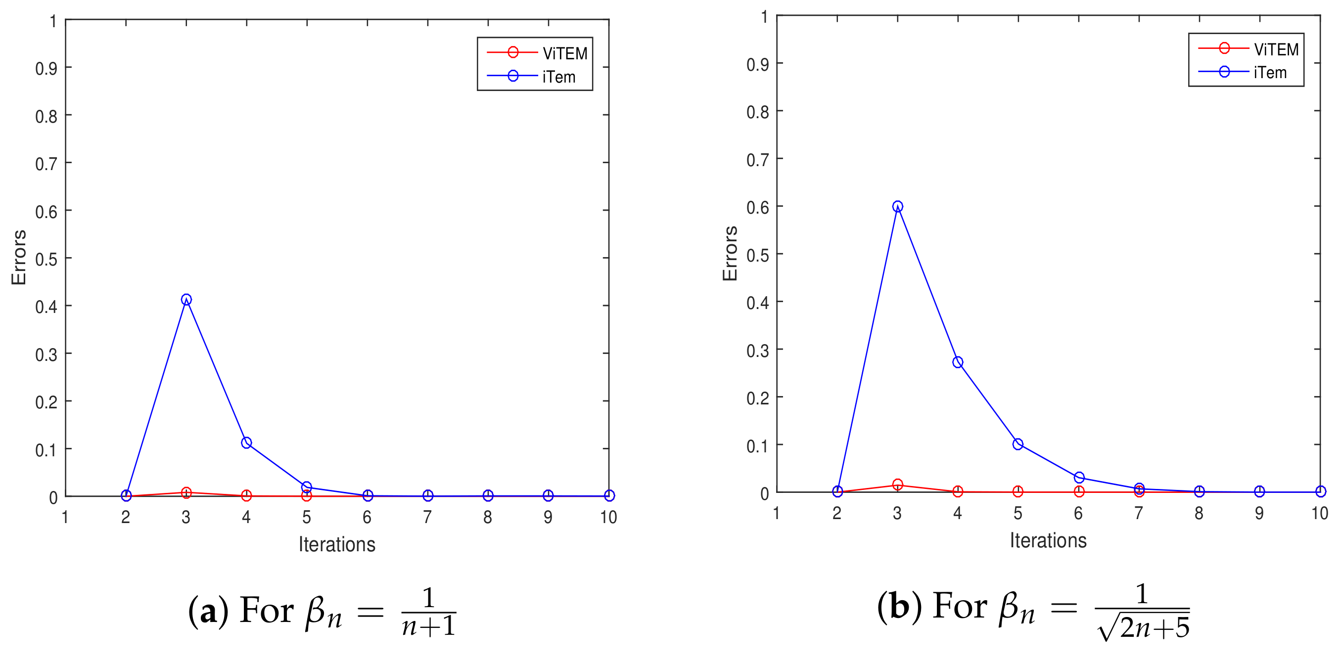
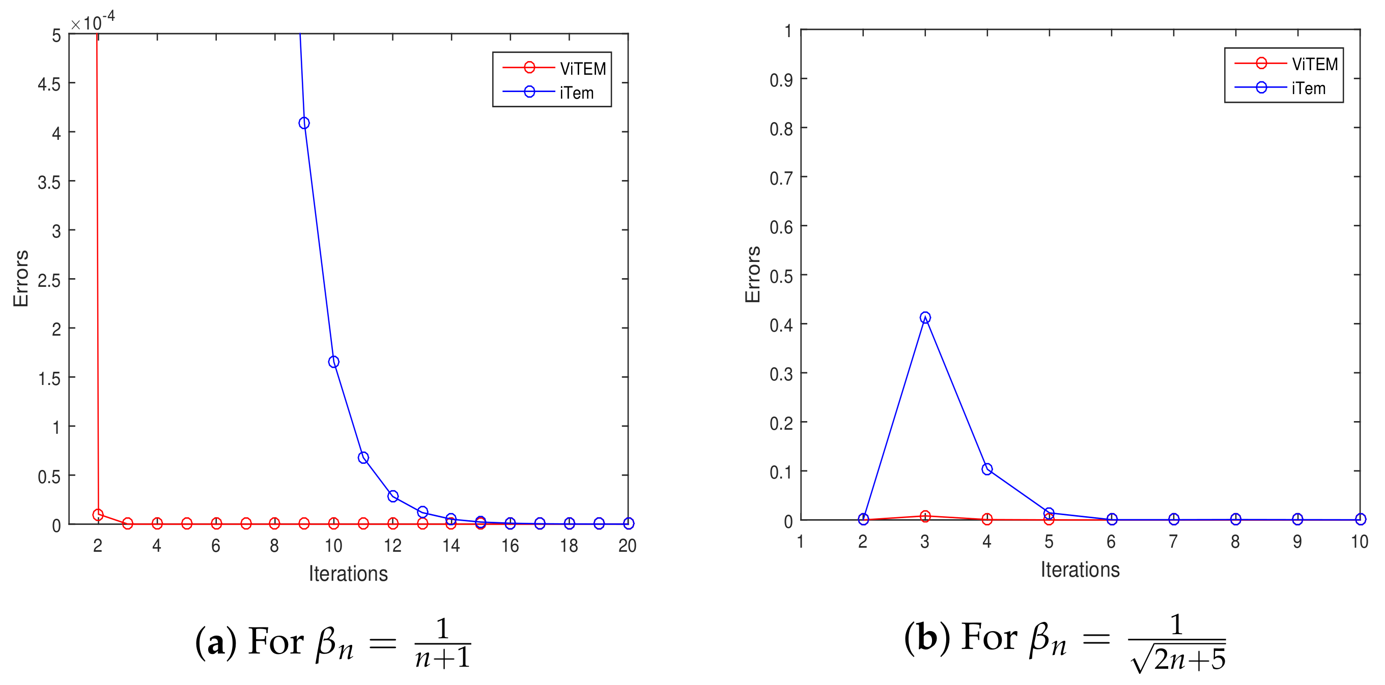
4. Numerical Illustrations

In this section, we provide some examples to illustrate and analyze the convergence of our proposed modified Tseng’s extragradient algorithm. In order to determine the execution time, we terminated the algorithm by using condition $\parallel x_{n+1}-x^{\ast }{\parallel }^2<ϵ$ where $x^{\ast }$ is the solution of the problem and $ϵ={10}^{-5}$.

Example 1.

Let $A:\mathbb{R}\to \mathbb{R}$ be defined by $Ax=2x.$ Clearly, A is monotone and Lipschitz continuous with $L=2$. Define $f:\mathbb{R}\to \mathbb{R}$ by $fx=\frac{x}{4}.$ Choose ${\alpha }_n=0.50$, ${\beta }_n=\frac{1}{n+2}$ and ${\theta }_n=0.5\ast (1-{\beta }_n)$ with $\lambda =0.4$. The feasible set is chosen to be $C=[-1,2]$.

Table 1. Comparison of elapsed CPU times.

	${\mathit{x}}_0=0.1$, ${\mathit{x}}_1=0.5$	${\mathit{x}}_0=0.5$, ${\mathit{x}}_1=1.5$
ViTEM	0.039508 s (iter = 5)	0.039197 s (iter = 5)
iTEM	0.040179 s (iter = 13)	0.040681 s (iter = 15)

below shows the comparison of elapsed times for the proposed algorithm ViTEM and iTEM [16]. We test the algorithms for two choices of initial points.

Figure 1 shows the comparison of two algorithms for different choices of parameter ${\beta }_n$. For this purpose, we chose $x_0=x_1=1$.

Example 2.

Define $A:{\mathbb{R}}^2\to {\mathbb{R}}^2$ by $A(x,y)=(x+y+sinx,-x+y+siny).$ Note that A is monotone and Lipschitz mapping with $L=3$. Let $f\left(x\right)=\frac{x}{8}$. The feasible set is chosen to be $C=[-1,-1]\times [2,2]$. We chose ${\alpha }_n=3$, ${\beta }_n=\frac{1}{n+2}$ and ${\theta }_n=0.5\ast (1-{\beta }_n)$ with $\lambda =\frac{1}{4}$.

Table 2. Comparison of elapsed CPU times.

	${\mathit{x}}_0={(1,1)}^{\mathit{T}}$, ${\mathit{x}}_1={(1.5,1.5)}^{\mathit{T}}$	${\mathit{x}}_0={(-0.5,0.5)}^{\mathit{T}}$, ${\mathit{x}}_1={(1,1)}^{\mathit{T}}$
ViTEM	0.078728 s (iter = 3)	0.073666 s (iter = 3)
iTEM	0.081701 s (iter = 15)	0.076256 s (iter = 15)

below analyzes the elapsed times of ViTEM and iTEM [16] for different choices of $x_0$ and $x_1$.

Figure 2 shows the comparison of two algorithms for different choices of parameter ${\beta }_n$. For this purpose, we chose $x_0={(-0.5,0.5)}^T$ and $x_1={(1,1)}^T$.

Example 3.

Let $H=L^2\left([0,1]\right)$ with the inner product $\langle x,y\rangle :={\int }_0^{1}x\left(t\right)y\left(t\right)dt$ and the induced norm $\parallel x\parallel =\sqrt{{\int }_0^1{\left|x\left(t\right)\right|}^{2}dt}$, for all $x,y\in H$. The operator $A:H\to H$ defined by $A\left(x\right(t\left)\right)=max\{0,x(t\left)\right\}$ for $t\in [0,1]$ is monotone and Lipschitz continuous on H with $L=1$. The feasible set is chosen to be the unit ball, $C:=\{x\in H:\parallel x\parallel \le 1\}$. We chose ${\alpha }_n=0.5$, ${\beta }_n=\frac{1}{n+2}$ and ${\theta }_n=0.5\ast (1-{\beta }_n)$ with $\lambda =\frac{1}{2}$.

Table 3. Comparison of elapsed CPU times.

	${\mathit{x}}_0\left(\mathit{t}\right)=\frac{\mathit{t}}{100}$, ${\mathit{x}}_1\left(\mathit{t}\right)=\frac{\mathit{t}}{10}$	${\mathit{x}}_0\left(\mathit{t}\right)=0.5(\mathit{t}+0.5cos\left(\mathit{t}\right))$, ${\mathit{x}}_1=\mathit{t}+0.5cos\left(\mathit{t}\right)$
ViTEM	0.022461 s (iter = 4)	0.190571 s (iter = 5)
iTEM	0.032179 s (iter > 100)	0.590528 s (iter > 100)

below examines the elapsed times of ViTEM and ITEM [16] for different choices of initial points $x_0$ and $x_1$.

Figure 3 shows the comparison of two algorithms for different choices of parameter ${\beta }_n$. For this purpose, we chose $x_0\left(t\right)=\frac{t}{100}$ and $x_1\left(t\right)=\frac{t}{10}$.

5. Conclusions

By combining the modified Tseng’s extragradient method [13], the viscosity method [30] and the Picard–Mann method [31], a new algorithm is proposed for solving variational inequality problems in real Hilbert spaces. It is worth mentioning that the proposed method requires the computation of only one projection onto the feasible set in each iteration. A strong convergence theorem for the proposed algorithm is obtained under certain mild conditions. It is shown that the proposed method performs better than some existing methods for solving variational inequality problems via several numerical examples.

References

1. Stampacchia, G. Formes bilineaires coercitives sur les ensembles convexes. C. R. Acad. Sci. 1964, 258, 4413–4416. [Google Scholar]
2. Kinderleh, D.; Stampacchia, G. An introduction to variational inequalities and their applications. SIAM Class. Appl. Math. 2000, CL31, 222–277. [Google Scholar]
3. Censor, Y.; Gibali, A.; Reich, S. The subgradient extragradient method for solving variational inequalities in Hilbert space. J. Optim. Theory Appl. 2011, 148, 318–335. [Google Scholar] [CrossRef] [PubMed] [Green Version]
4. Censor, Y.; Gibali, A.; Reich, S. Algorithms for the split variational inequality problem. Numer. Algorithm 2012, 59, 301–323. [Google Scholar] [CrossRef]
5. Khan, A.R.; Ugwunnadi, G.C.; Makukula, Z.G.; Abbas, M. Strong convergence of inertial subgradient extragradient method for solving variational inequality in Banach space. Carpathian J. Math. 2019, 35, 327–338. [Google Scholar] [CrossRef]
6. Maingé, P.E. Projected subgradient techniques and viscosity for optimization with variational inequality constraints. Eur. J. Oper. Res. 2010, 205, 501–506. [Google Scholar] [CrossRef]
7. Okeke, G.A.; Abbas, M.; de la Sen, M. Inertial subgradient extragradient methods for solving variational inequality problems and fixed point problems. Axioms 2020, 9, 51. [Google Scholar] [CrossRef]
8. Alber, Y.I.; Iusem, A.N. Extension of subgradient techniques for nonsmooth optimization in Banach spaces. Set-Valued Anal. 2001, 9, 315–335. [Google Scholar] [CrossRef]
9. Xiu, N.H.; Zhang, J.Z. Some recent advances in projection-type methods for variational inequalities. J. Comput. Appl. Math. 2003, 152, 559–587. [Google Scholar] [CrossRef] [Green Version]
10. Korpelevich, G.M. The extragradient method for finding saddle points and other problems. Ekon. Mat. Metod. 1976, 12, 747–756. [Google Scholar]
11. Antipin, A.S. On a method for convex programs using a symmetrical modification of the Lagrange function. Ekon. Mat. Metod. 1976, 12, 1164–1173. [Google Scholar]
12. Kraikaew, R.; Saejung, S. Strong convergence of the Halpern subgradient extragradient method for solving variational inequalities in Hilbert spaces. J. Optim. Theory Appl. 2014, 163, 399–412. [Google Scholar] [CrossRef]
13. Tseng, P. A modified forward-backward splitting method for maximal monotone mappings. SIAM J. Control Optim. 2000, 38, 431–446. [Google Scholar] [CrossRef]
14. Chen, J.; Liu, S.; Chang, X. Modified Tseng’s extragradient methods for variational inequality on Hadamard manifolds. Appl. Anal. 2021, 100, 2627–2640. [Google Scholar] [CrossRef]
15. Suantai, S.; Kankam, K.; Cholamjiak, P. A novel forward-backward algorithm for solving convex minimization problem in Hilbert spaces. Mathematics 2020, 8, 42. [Google Scholar] [CrossRef] [Green Version]
16. Thong, D.V.; Vinh, N.T.; Cho, Y.J. A strong convergence theorem for Tseng’s extragradient method for solving variational inequality problems. Optim. Lett. 2019, 14, 1157–1175. [Google Scholar] [CrossRef]
17. Attouch, H.; Goudon, X.; Redont, P. The heavy ball with friction. I. The continuous dynamical system. Commun. Contemp. Math. 2000, 2, 1–34. [Google Scholar] [CrossRef]
18. Attouch, H.; Czamecki, M.O. Asymptotic control and stabilization of nonlinear oscillators with non-isolated equilibria. J. Differ. Equ. 2002, 179, 278–310. [Google Scholar] [CrossRef] [Green Version]
19. Alvarez, F.; Attouch, H. An inertial proximal method for maximal monotone operators via discretization of a nonlinear oscillator with damping. Set-Valued Anal. 2001, 9, 3–11. [Google Scholar] [CrossRef]
20. Maingé, P.E. Inertial iterative process for fixed points of certain quasi-nonexpansive mappings. Set-Valued Anal. 2007, 15, 67–69. [Google Scholar] [CrossRef]
21. Maingé, P.E. Convergence theorems for inertial KM-type algorithms. J. Comput. Appl. Math. 2008, 219, 223–236. [Google Scholar] [CrossRef] [Green Version]
22. Ceng, L.C. Asymptotic inertial subgradient extragradient approach for pseudomonotone variational inequalities with fixed point constraints of asymptotically nonexpansive mappings. Commun. Optim. Theory 2020, 2020, 2. [Google Scholar]
23. Tian, M.; Xu, G. Inertial modified Tseng’s extragradient algorithms for solving monotone variational inequalities and fixed point problems. J. Nonlinear Funct. Anal. 2020, 2020, 35. [Google Scholar]
24. Attouch, H.; Peypouquet, J.; Redont, P. A dynamical approach to an inertial forward-backward algorithm for convex minimization. SIAM J. Optim. 2014, 24, 232–256. [Google Scholar] [CrossRef]
25. Bot, R.I.; Csetnek, E.R.; Hendrich, C. Inertial Douglas-Rachford splitting for monotone inclusion problems. Appl. Math. Comput. 2015, 256, 472–487. [Google Scholar]
26. Chen, C.; Chan, R.H.; Ma, S.; Yang, J. Inertial proximal ADMM for linearly constrained separable convex optimization. SIAM J. Imaging Sci. 2015, 8, 2239–2267. [Google Scholar] [CrossRef]
27. Bot, R.I.; Csetnek, E.R. A hybrid proximal-extragradient algorithm with inertial effects. Numer. Funct. Anal. Optim. 2015, 36, 951–963. [Google Scholar] [CrossRef] [Green Version]
28. Dong, L.Q.; Cho, Y.J.; Zhong, L.L.; Rassias, T.M. Inertial projection and contraction algorithms for variational inequalities. J. Glob. Optim. 2018, 70, 687–704. [Google Scholar] [CrossRef]
29. Bot, R.I.; Csetnek, E.R. An inertial forward-backward-forward primal-dual splitting algorithm for solving monotone inclusion problems. Numer. Algor. 2016, 71, 519–540. [Google Scholar] [CrossRef] [Green Version]
30. Moudafi, A. Viscosity approximations methods for fixed point problems. J. Math. Anal. Appl. 2000, 241, 46–55. [Google Scholar] [CrossRef] [Green Version]
31. Khan, S.H. A Picard-Mann hybrid iterative process. Fixed Point Theory Appl. 2013, 2013, 69. [Google Scholar] [CrossRef]
32. Goebel, K.; Reich, S. Uniform Convexity, Hyperbolic Geometry and Nonexpansive Mappings; Marcel Dekker: New York, NY, USA; Basel, Switzerland, 1984. [Google Scholar]
33. Kimura, Y.; Saejung, S. Strong convergence for a common fixed point of two different generalizations of cutter operators. Linear Nonlinear Anal. 2015, 1, 53–65. [Google Scholar]
34. Saejung, S.; Yotkaew, P. Approximation of zeros of inverse strongly monotone operators in Banach spaces. Nonlinear Anal. 2012, 75, 742–750. [Google Scholar] [CrossRef]
35. Suantai, S.; Pholasa, N.; Cholamjiak, P. The modified inertial relaxed CQ algorithm for solving the split feasibility problems. J. Ind. Manag. Optim. 2018, 14, 1595–1615. [Google Scholar] [CrossRef] [Green Version]
Figure 1. Comparison of convergence.
Axioms 10 00248 g001
Figure 2. Comparison of convergence.
Axioms 10 00248 g002
Figure 3. Comparison of convergence.
Axioms 10 00248 g003