Closure System and Its Semantics

Abstract

It is well known that topological spaces are axiomatically characterized by the topological closure operator satisfying the Kuratowski Closure Axioms. Equivalently, they can be axiomatized by other set operators encoding primitive semantics of topology, such as interior operator, exterior operator, boundary operator, or derived-set operator (or dually, co-derived-set operator). It is also known that a topological closure operator (and dually, a topological interior operator) can be weakened into generalized closure (interior) systems. What about boundary operator, exterior operator, and derived-set (and co-derived-set) operator in the weakened systems? Our paper completely answers this question by showing that the above six set operators can all be weakened (from their topological counterparts) in an appropriate way such that their inter-relationships remain essentially the same as in topological systems. Moreover, we show that the semantics of an interior point, an exterior point, a boundary point, an accumulation point, a co-accumulation point, an isolated point, a repelling point, etc. with respect to a given set, can be extended to an arbitrary subset system simply by treating the subset system as a base of a generalized interior system (and hence its dual, a generalized closure system). This allows us to extend topological semantics, namely the characterization of points with respect to an arbitrary set, in terms of both its spatial relations (interior, exterior, or boundary) and its dynamic convergence of any sequence (accumulation, co-accumulation, and isolation), to much weakened systems and hence with wider applicability. Examples from the theory of matroid and of Knowledge/Learning Spaces are used as an illustration.

1. Introduction

Let us recall the notions of topology and topological space [1,2,3]. A topology on a set X is a collection $\mathcal{T}$ of subsets of X, including the empty set ∅ and X itself, in which $\mathcal{T}$ is closed under arbitrary union and finite intersection; $(X,\mathcal{T})$ is then called a topological space. Those subsets of X, which are members of $\mathcal{T}$, are called open (sub)set in the space $(X,\mathcal{T})$. A subset $A\subseteq X$ is called closed in $(X,\mathcal{T})$ if its complement $X\backslash A\equiv A^c$ is an open set. From De Morgan’s Law, we infer that the collection of closed sets includes ∅ and X, and that such collection is closed under finite union and arbitrary intersection. So, specifying a collection of open sets amounts to specifying the collection of closed sets, and vice versa; this is the basic semantic duality. For this reason, whether the set system (i.e., a collection of subsets of X) $\mathcal{T}$ designates the collection of open sets or of closed sets is purely a choice of taste, by requiring the collection to be closed either in terms of “arbitrary union and finite intersection” (in the case of open sets) or “arbitrary intersection and finite union” (in the case of closed sets). We call it a topology. Note we say “a collection $\mathcal{T}$ is closed under ⋯” to mean that the result after the union/intersection operations is still a member of the collection. The clashing of meanings of the word “closed” with entirely different usages creates a cognitive burden most unfortunate for students of topology. For this reason, we sometime use the phrase “stable under” to describe “closed under.”

Associated with any topology $\mathcal{T}$ is the topological closure operator, denoted $\mathbf{Cl}$, which gives, for any subset $A\subseteq X$, the smallest closed set containing A. Obviously, a set A is closed if and only if $\mathbf{Cl}$$\left(A\right)=A$. Therefore, we can treat $\mathcal{T}$ as the collection of all fixed points of the $\mathbf{Cl}$ operator. Here and below, we call a set $A\subseteq X$ a fixed point of an operator $\mathbf{Op}$ if and only if $\mathbf{Op}$$\left(A\right)=A$.

Denote $\mathcal{P}\left(X\right)$ as the powerset of X. Then $\mathbf{Cl}$ as defined above is viewed as an operator $\mathbf{Cl}:\mathcal{P}\left(\mathbf{X}\right)\to \mathcal{P}\left(\mathbf{X}\right)$ that satisfies the following properties (for any sets $A,B\subseteq X$):

$\left[\mathrm{C}\mathrm{O}1\right]$$\mathbf{Cl}(\varnothing )=\varnothing$;

$\left[\mathrm{C}\mathrm{O}2\right]$$A\subseteq \mathbf{Cl}$$\left(A\right)$;

$\left[\mathrm{C}\mathrm{O}3\right]$$\mathbf{Cl}(\mathbf{Cl}$$\left(A\right))=\mathbf{Cl}$$\left(A\right)$;

$\left[\mathrm{C}\mathrm{O}4\right]$$\mathbf{Cl}$$(A\cup B)=\mathbf{Cl}$$\left(A\right)\cup \mathbf{Cl}$$\left(B\right)$.

Indeed, any operator $\mathbf{Cl}$ on $\mathcal{P}\left(X\right)$ that satisfies the above four axioms (called Kuratowski Closure Axioms) defines a topological closure operator. Its fixed points $\{A$$\mid \mathbf{Cl}$$\left(A\right)=A\}$ form a set system that can be properly identified as a collection of closed sets. We can then take set-complement of each of these closed sets to obtain another collection (i.e., another system of sets), which properly form an (open set) topology. In this sense, we can say that an operator satisfying the Kuratowski Closure Axioms $\left[\mathrm{C}\mathrm{O}1\right]$–$\left[\mathrm{C}\mathrm{O}4\right]$ defines a topological space $(X,\mathcal{T})$.

Dual to the topological closure operator is the topological interior operator $\mathbf{Int}$, which satisfies the following four axioms (for any sets $A,B\subseteq X$):

$\left[\mathrm{I}\mathrm{O}1\right]$$\mathbf{Int}$$\left(X\right)=X$;

$\left[\mathrm{I}\mathrm{O}2\right]$$\mathbf{Int}$$\left(A\right)\subseteq A$;

$\left[\mathrm{I}\mathrm{O}3\right]$$\mathbf{Int}(\mathbf{Int}$$\left(A\right))=\mathbf{Int}$$\left(A\right)$;

$\left[\mathrm{I}\mathrm{O}4\right]$$\mathbf{Int}$$(A\cap B)=\mathbf{Int}$$\left(A\right)\cap \mathbf{Int}$$\left(B\right)$.

The fixed points of $\mathbf{Int}$, the set system $\{A\mid$$\mathbf{Int}$$\left(A\right)=A\}$, form a system of subsets of X that will be called “open sets”, hence defining the topological space $(X,\mathcal{T})$. Here, “dual” in $\mathbf{Int}$ and $\mathbf{Cl}$ as operators is in the sense of basic semantic duality of “open” versus “closed” sets as their respective fixed points. Topological semantics of $\mathbf{Cl}$$\left(A\right)$ and $\mathbf{Int}$$\left(A\right)$ as they operate on an arbitrary subset $A\subseteq X$ are both consistent with their respective set of axioms defining the corresponding operator.

The equivalence of the above two axiomatically defined operators on $\mathcal{P}\left(X\right)$ in specifying any topology $\mathcal{T}$ is well known. In addition to the closure or interior operators defining a topological space, there are other four set operators widely used as primitive operators in topology. They are the exterior operator, the boundary operator, the derived-set operator, and the dually defined co-derived-set operator. All these operators have been shown to be able to specify an identical topology $\mathcal{T}$—they are equivalent to one another, as with $\mathbf{Cl}$ and $\mathbf{Int}$ operators. We call these various inter-related set operators specifying the one and the same topology a Topological System, while still use $(X,\mathcal{T})$ to denote it. Each of the six above-mentioned operators $\mathcal{P}\left(X\right)\to \mathcal{P}\left(X\right)$ provides equivalent characterizations of $(X,\mathcal{T})$. In a Topological System, the various operators, when taken together, provide comprehensive topological semantics to ground first-order modal logic.

In parallel to these various axiomatizations of a Topological System, it is also long established that the topological closure operator can be relaxed to the more general setting of a Closure System in which the closure operator satisfies, instead of $\left[\mathrm{C}\mathrm{O}1\right]$–$\left[\mathrm{C}\mathrm{O}4\right]$, three similar axioms (see below), without enforcing axiom $\left[\mathrm{C}\mathrm{O}1\right]$ (related to “groundedness”) and axiom $\left[\mathrm{C}\mathrm{O}4\right]$ (related to “stable under union”). The fixed points associated with this generalized closure operator are called (generalized) closed sets. Viewed in this way, the closed set system of a Topological System is just a special case of a generalized Closure System. Other applications of the Closure System include Matroid, Antimatroid/Learning Space [4,5,6,7], or Concept Lattice [8], in which the generalized closure operator is enhanced with an additional exchange axiom, anti-exchange axiom, or a Galois connection. Closure Systems also play an important role in Category Theory [9,10,11] and, particularly, in Category Topology [12,13], where the categorical closure operator studied are often not even required to satisfy the (categorical analogue of the) axiom $\left[\mathrm{C}\mathrm{O}3\right]$.

Given this theoretical backdrop, we can immediately ask whether there exist meaningful generalizations of the other five operators (interior, exterior, boundary, derived set, co-derived set) of a Topological System to any Closure System. Implicit in the “meaningfulness” is the requirement that these generalized operators would behave in a way that mirrors the respective roles of their topological counterparts. In other words, we require that the relations interlocking one operator to another be preserved. If a meaningful generalization can be achieved, then we can make the claim that the Closure System is indeed a strict weakening (i.e., less restrictive) of the Topological System with its semantics of the relevant operations nevertheless being preserved.

In the present work, we give a complete, positive answer to the above question. We provide the axiomatic systems for the suite of all six generalized operators. Some of the generalizations are straightforward, for instance, the generalized interior and generalized exterior operators are linked to the generalized closure operator in a direct way which involves only the set-complement operation. Generalization of other operators are more subtle, with much more involved work. We carefully analyze earlier axiomatization schemes for the topological boundary operator and for topological derived set operator [14,15,16,17], to obtain a generalization of boundary, derived set, and co-derived-set operators in the setting of Closure System, by appropriately relaxing the required axioms of the corresponding operators in the setting of Topological System. In this way, the relationships between these latter three operators themselves and their relationship with the closure/interior/exterior operators mimic those in the topological context. In doing so, we achieve a full axiomatic characterization of relevant operators in the (more general) Closure System.

The remaining part of the paper is organized as follows. Section 2 reviews the various axiomatizations of topological set operators—we highlight some important properties of the boundary operator and of the derived-set operator. In Section 3, starting from the known generalizations to the closure operator, interior operator, and exterior operator (Section 3.1), we provide a generalization of the boundary operator (Section 3.2), and a generalization of the derived-set operator (Section 3.3) and of the co-derived-set operator (Section 3.4). We describe the relationships of these operators (Section 3.5), as well as how a closure system may arise from Galois connections in general (Section 3.6). In Section 4, we elaborate on the semantics of various operators in terms of the points they characterize with respect to an arbitrary given set. There, from the more general subset system, we first induce an interior system (of open sets) and the system of subsets in the subset system as its “base”, and then show that the interior system is compatible with the derived-set operator defined on the same subset system (Section 4.1). Then the semantics of boundary points, accumulation points, co-accumulation points, repelling points, and isolated points of a subset system are provided (Section 4.2). Their classification into one of the exclusive categories and their inter-relationships with respect to a given set is summarized (Section 4.3). In Section 5, applications of our results to matroid and antimatroid (Section 5.1) and to the theory of Knowledge Space/Learning Space (Section 5.2) are demonstrated. We finish our paper with a short summary and conclusion (Section 6). We disclose here that a portion of our results (presented in Section 2 and Section 3) have been previously reported in conference proceedings format to the Eighth International Symposium of Domain Theory and Its Applications ISDT 2019 [18].

2. Equivalent Characterizations of a Topological System

Topological Systems are specified, equivalently, by either the collection of open sets, or the collection of closed sets as set systems. In addition to the topological closure and topological interior operators for characterizing a topology, there are four other operators commonly used in topology, namely exterior operator, boundary operator, derived-set operator, and co-derived-set operator. Each of these can also be used to completely characterize a Topological System, as shown by the work of [14,15,16,17,19]. The work of Zarycki [19], built on Kuratowski’s axiomatization of topological closure operator, axiomatized the topological exterior operator (denoted $\mathbf{Ext}$ below), the topological interior operator (denoted $\mathbf{Int}$ below), the topological boundary operator (denoted $\mathbf{Fr}$ below); these operators were independently reported by [14]. In Ref. [19], $\mathbf{Fr}$ is called a “frontier operator” while at the same time another “boundary” operator” $\mathbf{Br}$ is defined by $\mathbf{Br}\left(A\right)\equiv \mathbf{Fr}\left(A\right)\cap A$. In this way, the boundary region $\mathbf{Fr}\left(A\right)=\mathbf{Fr}\left(A^c\right)$ can be partitioned into two pieces: $\mathbf{Br}\left(A\right)=A\cap \mathbf{Fr}\left(A\right)$ and $\mathbf{Br}\left(A^c\right)=A^c\cap \mathbf{Fr}\left(A^c\right)$. (See Section 4.3 for more discussions.) The work of [15,17] further axiomatized the topological derived-set operator. We discuss these operators below.

2.1. Exterior Operator

We first discuss the exterior operator in a topological space. Given a topological interior operator $\mathbf{Int}:\mathcal{P}\left(\mathbf{X}\right)\to \mathcal{P}\left(\mathbf{X}\right)$, one can define the so-called topological exterior operator related to $\mathbf{Int}$ by $\mathbf{Ext}$$\left(A\right)=\mathbf{Int}$$\left(A^c\right)$ where $A^c\equiv X\backslash A$ denotes set-complement of A. Just as the set $\mathbf{Int}$$\left(A\right)$ gives the interior of A, the set $\mathbf{Ext}$$\left(A\right)$ gives the exterior of A in the topological space $(X,\mathcal{T})$.

The question of whether one can do the converse, namely axiomatically characterize $\mathbf{Ext}$ as a primitive operator from which $\mathbf{Cl}$ and $\mathbf{Int}$ operators are derived from, was answered affirmatively first by Zarycki [19] and then reported by Gabai [14] nearly half a century later. In other words, one can specify the Topological System by a topological exterior operator $\mathbf{Ext}$ axiomatically defined as follows.

Definition 1.

(Topological Exterior Operator).

An operator $\mathbf{Ext}$: $\mathcal{P}\left(X\right)\to \mathcal{P}\left(X\right)$ is called a topological exterior operator if for any sets $A,B\subseteq X$, $\mathbf{Ext}$ satisfies the following four axioms:

$\left[\mathrm{E}\mathrm{O}1\right]$$\mathbf{Ext}$$(\varnothing )=X$;

$\left[\mathrm{E}\mathrm{O}2\right]$$A\cap \mathbf{Ext}$$\left(A\right)=\varnothing$;

$\left[\mathrm{E}\mathrm{O}3\right]$$\mathbf{Ext}$$(X\backslash \mathbf{Ext}$$\left(A\right))=\mathbf{Ext}$$\left(A\right)$;

$\left[\mathrm{E}\mathrm{O}4\right]$$\mathbf{Ext}$$(A\cup B)=\mathbf{Ext}$$\left(A\right)\cap \mathbf{Ext}$$\left(B\right)$.

Given an operator $\mathbf{Ext}$ satisfying the above four axioms, then we can obtain the collection $\mathcal{T}=\{E\in \mathcal{P}(X)\mid \mathbf{Ext}$$(X\backslash E)=E\}=\{E\in \mathcal{P}\left(X\right)\mid \mathbf{Ext}$$\left(E^c\right)=E\}$, which turns out to define a Topological System. Moreover, $\mathcal{T}$ will define the only open set topology that is compatible with the “exterior” semantic of this operator $\mathbf{Ext}$, i.e., an operator complementary to the interior operator whose fixed points forms the system of open sets of $\mathcal{T}$.

Note that the three topological operators $\mathbf{Ext}$, $\mathbf{Int}$, and $\mathbf{Cl}$ are related to one another by the following relations:

$$\mathbf{Int}\left(A\right)=\mathbf{Ext}\left(A^c\right)⟺\mathbf{Int}\left(A^c\right)=\mathbf{Ext}\left(A\right);$$

$$\mathbf{Cl}\left(A\right)=(\mathbf{Ext}{\left(A\right))}^c⟺(\mathbf{Cl}{\left(A\right))}^c=\mathbf{Ext}\left(A\right);$$

$$\mathbf{Cl}\left(A\right)=(\mathbf{Int}\left(A^c\right){)}^c⟺\mathbf{Cl}\left(A^c\right)=(\mathbf{Int}{\left(A\right))}^c.$$

2.2. Boundary Operator

In addition to $\mathbf{Ext}$, the work of [14,19] also axiomatized the so-called topological boundary operator. The system used by [14] is given below; Ref. [19] used $\left[\mathrm{F}\mathrm{O}1\right]$, $\left[\mathrm{F}\mathrm{O}2\right]$, $\left[\mathrm{F}\mathrm{O}4\right]$ plus another axiom in place of $\left[\mathrm{F}\mathrm{O}5\right]$.

Definition 2.

(Topological Boundary Operator).

An operator $\mathbf{Fr}$: $\mathcal{P}\left(X\right)\to \mathcal{P}\left(X\right)$ is called a topological boundary (or frontier) operator if for any sets $A,B\subseteq X$, $\mathbf{Fr}$ satisfies the following five axioms:

$\left[\mathrm{F}\mathrm{O}1\right]$$\mathbf{Fr}$$(\varnothing )=\varnothing$;

$\left[\mathrm{F}\mathrm{O}2\right]$$\mathbf{Fr}$$\left(A\right)=\mathbf{Fr}$$\left(A^c\right)$;

$\left[\mathrm{F}\mathrm{O}3\right]$$A\subseteq B\Rightarrow \mathbf{Fr}$$\left(A\right)\subseteq B\cup \mathbf{Fr}$$\left(B\right)$;

$\left[\mathrm{F}\mathrm{O}4\right]$$\mathbf{Fr}$$(\mathbf{Fr}$$\left(A\right))\subseteq \mathbf{Fr}$$\left(A\right)$;

$\left[\mathrm{F}\mathrm{O}5\right]$$\mathbf{Fr}$$(A\cup B)\subseteq \mathbf{Fr}$$\left(A\right)\cup \mathbf{Fr}$$\left(B\right)$.

Note that axiom $\left[\mathrm{F}\mathrm{O}2\right]$ dictates that the boundary $\mathbf{Fr}$$\left(A\right)$ of A is the same as the boundary $\mathbf{Fr}$$\left(A^c\right)$ of $A^c$; in other words, A and $A^c\equiv X\backslash A$ share the “common” boundary points.

With respect to a boundary (also called frontier) operator $\mathbf{Fr}$, we can construct $\mathcal{T}=\{E\in \mathcal{P}(X)\mid \mathbf{Fr}$$\left(E^c\right)\subseteq E^c\}$. The collection $\mathcal{T}$ so constructed is a topology. For $A\subseteq X$, $\mathbf{Fr}$$\left(A\right)$ is the boundary of A in the topological space $(X,\mathcal{T})$. Moreover, $\mathcal{T}$ is the only topology with the given boundary structure.

We now investigate the role of axiom $\left[\mathrm{F}\mathrm{O}5\right]$, the axiom to be removed when relaxing to a generalized Closure System.

Proposition 1.

 

$\left[\mathrm{F}\mathrm{O}4\right]$ and $\left[\mathrm{F}\mathrm{O}5\right]$ imply

${\left[\mathrm{F}\mathrm{O}4\right]}^{\ast }$$\mathbf{Fr}$$(A\cup \mathbf{Fr}$$\left(A\right))\subseteq \mathbf{Fr}$$\left(A\right)$,

which then implies $\mathbf{Fr}$$(A\cup \mathbf{Fr}$$\left(A\right))\subseteq A\cup \mathbf{Fr}$$\left(A\right)$.

Proof. 

By $\left[\mathrm{F}\mathrm{O}5\right],$ $\mathbf{Fr}$$(A\cup \mathbf{Fr}$$\left(A\right))\subseteq \mathbf{Fr}$$\left(A\right)\cup \mathbf{Fr}(\mathbf{Fr}$$\left(A\right)).$ Because of $\left[\mathrm{F}\mathrm{O}4\right]$, $\mathbf{Fr}$$\left(A\right)\cup \mathbf{Fr}(\mathbf{Fr}$$\left(A\right))=\mathbf{Fr}$$\left(A\right).$ Then $\mathbf{Fr}$$(A\cup \mathbf{Fr}$$\left(A\right))\subseteq \mathbf{Fr}$$\left(A\right)$ holds. Obviously, $\mathbf{Fr}$$(A\cup \mathbf{Fr}$$\left(A\right))\subseteq A\cup \mathbf{Fr}$$\left(A\right)$ also holds. □

If we drop axiom $\left[\mathrm{F}\mathrm{O}5\right]$ in the definition of $\mathbf{Fr}$, we do not have ${\left[\mathrm{F}\mathrm{O}4\right]}^{\ast }$. On the other hand, we have the following result.

Proposition 2.

 

$\left[\mathrm{F}\mathrm{O}2\right]$, $\left[\mathrm{F}\mathrm{O}3\right]$ and ${\left[\mathrm{F}\mathrm{O}4\right]}^{\ast }$ implies $\left[\mathrm{F}\mathrm{O}4\right]$.

Proof. 

Suppose a set operator $\mathbf{Fr}$ only satisfies $\left[\mathrm{F}\mathrm{O}2\right]$ and $\left[\mathrm{F}\mathrm{O}3\right]$ in Definition 2. For any $A\subseteq X$, $\mathbf{Fr}$$\left(A\right)\subseteq A\cup \mathbf{Fr}$$\left(A\right)$. An application of $\left[\mathrm{F}\mathrm{O}3\right]$ gives $\mathbf{Fr}$$(\mathbf{Fr}$$\left(A\right))\subseteq A\cup \mathbf{Fr}$$\left(A\right)\cup \mathbf{Fr}$$(A\cup \mathbf{Fr}$$\left(A\right))=A\cup \mathbf{Fr}$$\left(A\right)$, where the last step invokes ${\left[\mathrm{F}\mathrm{O}4\right]}^{\ast }$. Then $\mathbf{Fr}$$(\mathbf{Fr}$$\left(A\right))\subseteq A\cup \mathbf{Fr}$$\left(A\right)$ holds. Likewise, for the complement $X^c\equiv X\backslash A$, $\mathbf{Fr}$$(\mathbf{Fr}$$\left(A^c\right))\subseteq A^c\cup \mathbf{Fr}$$\left(A^c\right)$ holds. By $\left(\mathrm{F}\mathrm{O}2\right)$, we have $\mathbf{Fr}$$(\mathbf{Fr}$$\left(A\right))\subseteq A\cup \mathbf{Fr}$$\left(A\right)$ and $\mathbf{Fr}$$(\mathbf{Fr}$$\left(A\right))\subseteq A^c\cup \mathbf{Fr}$$\left(A\right)$. Therefore, $\mathbf{Fr}$$(\mathbf{Fr}$$\left(A\right))\subseteq (A\cup \mathbf{Fr}$$\left(A\right))\cap (A^c\cup \mathbf{Fr}$$\left(A\right))=(A\cap A^c)\cup \mathbf{Fr}$$\left(A\right))=\varnothing \cup \mathbf{Fr}$$\left(A\right)=\mathbf{Fr}$$\left(A\right)$, i.e., $\mathbf{Fr}$$(\mathbf{Fr}$$\left(A\right))\subseteq \mathbf{Fr}$$\left(A\right)$. □

From the above two Propositions, it follows that axiom $\left[\mathrm{F}\mathrm{O}4\right]$ in the axiomatic definition of $\mathbf{Fr}$ can be equivalently replaced by ${\left[\mathrm{F}\mathrm{O}4\right]}^{\ast }$. Then we have an alternative axiomatization of topological boundary operator $\mathbf{Fr}$.

Definition 3.

(Topological Boundary Operator, Alternative Definition).

An operator $\mathbf{Fr}$: $\mathcal{P}\left(X\right)\to \mathcal{P}\left(X\right)$ is called a topological boundary operator if for any sets $A,B\subseteq X$, $\mathbf{Fr}$ satisfies the following five axioms:

$\left[\mathrm{F}\mathrm{O}1\right]$$\mathbf{Fr}$$(\varnothing )=\varnothing$;

$\left[\mathrm{F}\mathrm{O}2\right]$$\mathbf{Fr}$$\left(A\right)=\mathbf{Fr}$$\left(A^c\right)$;

$\left[\mathrm{F}\mathrm{O}3\right]$$A\subseteq B\Rightarrow \mathbf{Fr}$$\left(A\right)\subseteq B\cup \mathbf{Fr}$$\left(B\right)$;

${\left[\mathrm{F}\mathrm{O}4\right]}^{\ast }$$\mathbf{Fr}$$(A\cup \mathbf{Fr}$$\left(A\right))\subseteq \mathbf{Fr}$$\left(A\right)$;

$\left[\mathrm{F}\mathrm{O}5\right]$$\mathbf{Fr}$$(A\cup B)\subseteq \mathbf{Fr}$$\left(A\right)\cup \mathbf{Fr}$$\left(B\right)$.

It is possible to further partition $\mathbf{Fr}\left(A\right)$ into two non-intersecting sets, $A\cap \mathbf{Fr}\left(A\right)$ and $A^c\cap \mathbf{Fr}\left(A\right)$. See discussions in the first paragraph of Section 2.

2.3. Derived-Set Operator

We will now turn to the derived-set operator and the co-derived-set operator. Derived set arises out of studying the limit points (called accumulation points, see Section 4.2.2) of topologically converging sequences. Harvey [17] and Spira [15] provided separate schemes for axiomatizing the derived-set operator in topological spaces. We follow the scheme by Harvey.

Definition 4.

(Topological Derived-Set Operator).

An operator $\mathbf{Der}$: $\mathcal{P}\left(X\right)\to \mathcal{P}\left(X\right)$ is called a topological derived-set operator if for any sets $A,B\subseteq X$, $\mathbf{Der}$ satisfies the following four axioms:

$\left[\mathrm{D}\mathrm{O}1\right]$$\mathbf{Der}$$(\varnothing )=\varnothing$;

$\left[\mathrm{D}\mathrm{O}2\right]$$x\in \mathbf{Der}$$\left(A\right)⟺x\in \mathbf{Der}$$(A\backslash \{x\left\}\right)$;

$\left[\mathrm{D}\mathrm{O}3\right]$$\mathbf{Der}$$(A\cup \mathbf{Der}$$\left(A\right))\subseteq A\cup \mathbf{Der}$$\left(A\right)$;

$\left[\mathrm{D}\mathrm{O}4\right]$$\mathbf{Der}$$(A\cup B)=\mathbf{Der}$$\left(A\right)\cup \mathbf{Der}$$\left(B\right)$.

Proposition 3.

 

A topological derived-set operator $\mathbf{Der}$ has the following property:

$\left[\mathrm{D}\mathrm{O}3\right]$${}^{\ast }$$\mathbf{Der}$$(\mathbf{Der}$$\left(A\right))\subseteq A\cup \mathbf{Der}$$\left(A\right)$ for any $A\subseteq X$.

Moreover, $\left[\mathrm{D}\mathrm{O}3\right]$${}^{\ast }$ is equivalent to $\left[\mathrm{D}\mathrm{O}3\right]$ under $\left[\mathrm{D}\mathrm{O}4\right]$.

Proof. 

First, we show that the topological derived-set operator $\mathbf{Der}$ is monotone: for any $A,B\subseteq X$, $A\subseteq B$ implies $\mathbf{Der}$$\left(A\right)\subseteq \mathbf{Der}$$\left(B\right)$. By $\left[\mathrm{D}\mathrm{O}4\right]$ and assuming $A\subseteq B$, $\mathbf{Der}$$(A\cup B)=\mathbf{Der}$$\left(B\right)=\mathbf{Der}$$\left(A\right)\cup \mathbf{Der}$$\left(B\right)$, which implies $\mathbf{Der}$$\left(A\right)\subseteq \mathbf{Der}$$\left(B\right)$.

For any $A\subseteq X$, $\mathbf{Der}$$\left(A\right)\subseteq A\cup \mathbf{Der}$$\left(A\right)$ holds. By the monotone property of $\mathbf{Der}$ and $\left[\mathrm{D}\mathrm{O}3\right]$, we have $\mathbf{Der}(\mathbf{Der}$$\left(A\right))\subseteq \mathbf{Der}$$(A\cup \mathbf{Der}$$\left(A\right))\subseteq A\cup \mathbf{Der}$$\left(A\right)$. Then $\mathbf{Der}$$(\mathbf{Der}$$\left(A\right))\subseteq A\cup \mathbf{Der}$$\left(A\right)$, so $\left[\mathrm{D}\mathrm{O}3\right]$${}^{\ast }$ holds.

On the other hand, suppose $\mathbf{Der}$ only satisfies $\left[\mathrm{D}\mathrm{O}4\right]$: $\mathbf{Der}$$(A\cup B)=\mathbf{Der}$$\left(A\right)\cup \mathbf{Der}$$\left(B\right)$. Then $\mathbf{Der}$$(A\cup \mathbf{Der}$$\left(A\right))=\mathbf{Der}$$\left(A\right)\cup \mathbf{Der}(\mathbf{Der}$$\left(A\right))$. By $\left[\mathrm{D}\mathrm{O}3\right]$${}^{\ast }$, $\mathbf{Der}$$(A\cup \mathbf{Der}$$\left(A\right))\subseteq A\cup \mathbf{Der}$$\left(A\right)$, i.e., $\left[\mathrm{D}\mathrm{O}3\right]$ holds. Therefore, $\left[\mathrm{D}\mathrm{O}3\right]$${}^{\ast }$ is equivalent to $\left[\mathrm{D}\mathrm{O}3\right]$ under $\left[\mathrm{D}\mathrm{O}4\right]$. □

From the above proposition, it follows that we can equivalently substitute $\left[\mathrm{D}\mathrm{O}3\right]$${}^{\ast }$ for $\left[\mathrm{D}\mathrm{O}3\right]$ in the definition of $\mathbf{Der}$. Denote

${\left[\mathrm{D}\mathrm{O}2\right]}^{\ast }$$x\notin \mathbf{Der}$($\left\{x\right\})$ for any $x\in X$.

Spira [15] showed that axiom $\left[\mathrm{D}\mathrm{O}2\right]$ is equivalent to ${\left[\mathrm{D}\mathrm{O}2\right]}^{\ast }$ under axioms $\left[\mathrm{D}\mathrm{O}1\right]$ and $\left[\mathrm{D}\mathrm{O}4\right]$. Therefore, we have an alternative, simpler axiomatic version for topological derived-set operator.

Definition 5.

(Topological Derived-Set Operator, Alternative Definition).

An operator $\mathbf{Der}$: $\mathcal{P}\left(X\right)\to \mathcal{P}\left(X\right)$ is called a topological derived-set operator if for any sets $A,B\subseteq X$, $\mathbf{Der}$ satisfies the following four axioms:

$\left[\mathrm{D}\mathrm{O}1\right]$$\mathbf{Der}$$(\varnothing )=\varnothing$;

${\left[\mathrm{D}\mathrm{O}2\right]}^{\ast }$ For any $x\in X$, $x\notin \mathbf{Der}$$\left(\right\{x\left\}\right)$;

${\left[\mathrm{D}\mathrm{O}3\right]}^{\ast }$$\mathbf{Der}$$(\mathbf{Der}$$\left(A\right))\subseteq A\cup \mathbf{Der}$$\left(A\right)$;

$\left[\mathrm{D}\mathrm{O}4\right]$$\mathbf{Der}$$(A\cup B)=\mathbf{Der}$$\left(A\right)\cup \mathbf{Der}$$\left(B\right)$.

2.4. Co-Derived-Set Operator

From a derived-set operator $\mathbf{Der}$, we can dually define an operator $\mathbf{Cod}$ through complementation: for any $A\subseteq X$, $\mathbf{Cod}$$\left(A\right)=(\mathbf{Der}$$\left(A^c\right){)}^c$. Equivalently, $\mathbf{Der}$$\left(A\right)=(\mathbf{Cod}$$\left(A^c\right){)}^c$. Steinsvold [16] used the co-derived-set operator as the semantics for belief in his Ph.D. Thesis.

Definition 6.

(Topological Co-Derived-Set Operator).

An operator $\mathbf{Cod}$: $\mathcal{P}\left(X\right)\to \mathcal{P}\left(X\right)$ is called a topological co-derived-set operator if for any sets $A,B\subseteq X$, $\mathbf{Cod}$ satisfies the following four axioms:

$\left[\mathrm{C}\mathrm{D}1\right]$$\mathbf{Cod}$$\left(X\right)=X$;

$\left[\mathrm{C}\mathrm{D}2\right]$$x\in \mathbf{Cod}$$\left(A\right)⟺x\in \mathbf{Cod}$$(A\cup \{x\left\}\right)$;

$\left[\mathrm{C}\mathrm{D}3\right]$$\mathbf{Cod}$$(A\cap \mathbf{Cod}$$\left(A\right))\supseteq A\cap \mathbf{Cod}$$\left(A\right)$;

$\left[\mathrm{C}\mathrm{D}4\right]$$\mathbf{Cod}$$(A\cap B)=\mathbf{Cod}$$\left(A\right)\cap \mathbf{Cod}$$\left(B\right)$.

Both derived set and co-derived set can be used to define a topology. Any subset $A\subseteq X$ is stipulated as being closed when $\mathbf{Der}$$\left(A\right)\subseteq A$. Then the collection $\mathcal{T}=\{E\in \mathcal{P}\left(X\right)\mid E^c$ is closed $\}=\{E\in \mathcal{P}\left(X\right)\mid \mathbf{Der}$$\left(E^c\right)\subseteq E^c\}$ will specify a Topological System on X, with the derived-set operator induced by $\mathcal{T}$ being just $\mathbf{Der}$. Moreover, $\mathcal{T}$ is the only topology satisfying this condition. Dually, $\widehat{\mathcal{T}}=\{E\in \mathcal{P}\left(X\right)\mid E\subseteq \mathbf{Cod}$$\left(E\right)\}$ also specifies a Topological System on X. The above two topological systems are indeed identical, i.e., $\mathcal{T}=\widehat{\mathcal{T}}$. So, a derived-set operator and its dual co-derived-set operator generate the same topology.

Up till this point, we see that a Topological System can be uniquely specified by any of the following six operators: $\mathbf{Cl},\mathbf{Int},\mathbf{Ext},\mathbf{Fr},\mathbf{Der},\mathbf{Cod}.$ These six operators, with their respective set of axioms, are rigidly interlocked.

3. Equivalent Characterizations of a Closure System

In this Section, we first review the relaxation from a topological closure operator (in a Topological System) to a generalized closure operator (in a Closure System), also denoted $\mathbf{Cl}$ here. We use the terminology Closure System to refer to the set system associated with this generalized closure operator (and related operators) to be discussed below, and reserve the terminology Topological System to refer exclusively to the topology (in the usual sense) characterized by a topological closure operator (and related operators) discussed in Section 2.

To study a Closure System, we start with the generalized closure operator. It turns out that in analogous to the situation of a Topological System, the three axioms for a generalized closure operator $\mathbf{Cl}$ can turn equivalently to an axiom system for a generalized interior operator $\mathbf{Int}$ and an axiom system for a generalized exterior operator $\mathbf{Ext}$. Note that all operators treated from now on refer to the “generalized” version, despite using the same bold-face symbols (and sometimes omitting the word “generalized”).

3.1. Generalized Closure, Interior, and Exterior Operators

We first recall the standard definition of a generalized closure operator.

Definition 7.

(Closure Operator).

An operator $\mathbf{Cl}$: $\mathcal{P}\left(X\right)\to \mathcal{P}\left(X\right)$ is called a generalized closure operator (or simply, closure operator) if for any sets $A,B\subseteq X$, $\mathbf{Cl}$ satisfies the following three axioms:

$\left[\mathrm{C}1\right]$$A\subseteq \mathbf{Cl}$$\left(A\right)$;

$\left[\mathrm{C}2\right]$$A\subseteq B\Rightarrow \mathbf{Cl}$$\left(A\right)\subseteq \mathbf{Cl}$$\left(B\right)$;

$\left[\mathrm{C}3\right]$$\mathbf{Cl}(\mathbf{Cl}$$\left(A\right))=\mathbf{Cl}$$\left(A\right)$.

Dually, we also have the axiomatic definition of a generalized interior operator, which is also well known.

Definition 8.

(Interior Operator).

An operator $\mathbf{Int}$: $\mathcal{P}\left(X\right)\to \mathcal{P}\left(X\right)$ is called the generalized interior operator (or simply, interior operator) if for any sets $A,B\subseteq X$, $\mathbf{Int}$ satisfies the following three axioms:

$\left[\mathrm{I}1\right]$$\mathbf{Int}$$\left(A\right)\subseteq A$;

$\left[\mathrm{I}2\right]$$A\subseteq B\Rightarrow \mathbf{Int}$$\left(A\right)\subseteq \mathbf{Int}$$\left(B\right)$;

$\left[\mathrm{I}3\right]$$\mathbf{Int}(\mathbf{Int}$$\left(A\right))=\mathbf{Int}$$\left(A\right)$.

The interior operator $\mathbf{Int}$ is dual to the closure operator $\mathbf{Cl}$, in the sense that for any $A\subset X$, $\mathbf{Int}$$\left(A\right)=(\mathbf{Cl}$$\left(A^c\right){)}^c$ and $\mathbf{Cl}$$\left(A\right)=(\mathbf{Int}$$\left(A^c\right){)}^c$.

In light of the identity between an exterior operator and an interior operator operating on any subset A of X: $\mathbf{Int}$$\left(A\right)\equiv \mathbf{Ext}$$\left(A^c\right)$, the axiomatic definition of a generalized exterior operator is obtained (in analogous to how the topological exterior operator is defined in relation to the definitions of topological closure and topological interior operators) as follows.

Definition 9.

(Exterior Operator).

An operator $\mathbf{Ext}$: $\mathcal{P}\left(X\right)\to \mathcal{P}\left(X\right)$ is called a generalized exterior operator (or simply, exterior operator) if for any sets $A,B\subseteq X$, $\mathbf{Ext}$ satisfies the following three axioms:

$\left[\mathrm{E}1\right]$$A\cap \mathbf{Ext}$$\left(A\right)=\varnothing$;

$\left[\mathrm{E}2\right]$$A\subseteq B\Rightarrow \mathbf{Ext}$$\left(A\right)\supseteq \mathbf{Ext}$$\left(B\right)$;

$\left[\mathrm{E}3\right]$$\mathbf{Ext}$$(X\backslash \mathbf{Ext}$$\left(A\right))=\mathbf{Ext}$$\left(A\right)$.

3.2. Generalized Boundary Operator

We now turn to generalized boundary (or frontier) operator. A careful comparison of how a topological closure operator can be relaxed to become a generalized closure operator, we see that $\left[\mathrm{F}\mathrm{O}1\right]$ and $\left[\mathrm{F}\mathrm{O}5\right]$ in the definition of topological boundary operator can be dropped to obtain a generalized boundary operator. $\left[\mathrm{F}\mathrm{O}2\right]$ expresses the essence of “boundary” (or “frontier”) of a closed set. $\left[\mathrm{F}\mathrm{O}3\right]$ shows $\mathbf{Fr}$ is “monotone” in some sense. ${\left[\mathrm{F}\mathrm{O}4\right]}^{\ast }$ corresponds to the “idempotency” of the closure operator. Therefore, we only retain $\left[\mathrm{F}\mathrm{O}2\right]$, $\left[\mathrm{F}\mathrm{O}3\right]$ and ${\left[\mathrm{F}\mathrm{O}4\right]}^{\ast }$ to obtain the definition of generalized boundary operator.

Definition 10.

(Boundary Operator).

An operator $\mathbf{Fr}$: $\mathcal{P}\left(X\right)\to \mathcal{P}\left(X\right)$ is called a generalized boundary operator (or simply, boundary operator) if for any sets $A,B\subseteq X$, $\mathbf{Fr}$ satisfies the following three axioms:

$\left[\mathrm{F}1\right]$$\mathbf{Fr}$$\left(A\right)=\mathbf{Fr}$$(X\backslash A)$;

$\left[\mathrm{F}2\right]$$A\subseteq B\Rightarrow \mathbf{Fr}$$\left(A\right)\subseteq B\cup \mathbf{Fr}$$\left(B\right)$;

$\left[\mathrm{F}3\right]$$\mathbf{Fr}$$(A\cup \mathbf{Fr}$$\left(A\right))\subseteq \mathbf{Fr}$$\left(A\right)$.

Proposition 4.

 

The boundary operator $\mathbf{Fr}$ has the following property:

${\left[\mathrm{F}3\right]}^{\ast }$$\mathbf{Fr}$$(\mathbf{Fr}$$\left(A\right))\subseteq \mathbf{Fr}$$\left(A\right)$ for any $A\subseteq X$.

Proof. 

See the proof of Proposition 2. □

As we recall, ${\left[\mathrm{F}3\right]}^{\ast }$ as stated above is axiom $\left[\mathrm{F}\mathrm{O}4\right]$ in the topological boundary operator. However, ${\left[\mathrm{F}3\right]}^{\ast }$ cannot be an alternative axiom in the definition of generalized boundary operator. In fact, ${\left[\mathrm{F}3\right]}^{\ast }$ is strictly weaker than $\left[\mathrm{F}3\right]$ under $\left[\mathrm{F}1\right]$ and $\left[\mathrm{F}2\right]$. It can be seen from the following example.

Example 1.

Let $X=\{1,2,3\}$. Define an operator $\mathbf{Fr}$ by

$\mathbf{Fr}$$\left(A\right)=\left\{\begin{array}{ccc}\varnothing & A=\varnothing or X,\hfill & \\ \left\{2\right\}& A=\left\{1\right\} or \{2,3\} or \left\{2\right\} or \{1,3\},\hfill & \\ \left\{3\right\}& A=\left\{3\right\} or \{1,2\}.\hfill \end{array}\right.$

$\mathbf{Fr}$ satisfies $\left[\mathrm{F}1\right]$, $\left[\mathrm{F}2\right]$, and ${\left[\mathrm{F}3\right]}^{\ast }$. However, $\mathbf{Fr}$ does not satisfy axiom $\left[\mathrm{F}3\right]$: for $A=\left\{1\right\}$, $\mathbf{Fr}$$\left(A\right)=\left\{2\right\}$, $\mathbf{Fr}$$(A\cup \mathbf{Fr}$$\left(A\right))=\mathbf{Fr}$$\left(\right\{1,2\left\}\right)=\left\{3\right\}$. Obviously, $\mathbf{Fr}$$(A\cup \mathbf{Fr}$$\left(A\right))⊈\mathbf{Fr}$$\left(A\right)$.

Boundary operators and closure operators have a one-to-one correspondence in Topological Systems. Likewise, for their generalizations in Closure Systems, we expect such correspondence to still hold.

Theorem 1.

(From $\mathbf{Fr}$ to $\mathbf{Cl}$).

Let $\mathbf{Fr}$: $\mathcal{P}\left(X\right)\to \mathcal{P}\left(X\right)$ be a boundary operator. Define the operator $\mathbf{Cl}$ as $\mathbf{Cl}$$\left(A\right)=:A\cup \mathbf{Fr}$$\left(A\right)$ for any subset A of X. Then $\mathbf{Cl}$ as defined is a (generalized) closure operator.

Proof. 

To prove $\left[\mathrm{C}1\right]$, for any subset A of X, we have $A\subseteq A\cup \mathbf{Fr}$$\left(A\right)=$$\mathbf{Cl}$$\left(A\right)$, where the last step is by our definition of the operator $\mathbf{Cl}$. Therefore, $A\subseteq \mathbf{Cl}$$\left(A\right)$.

To prove $\left[\mathrm{C}2\right]$, given $A\subseteq B\subseteq X$, axiom $\left[\mathrm{F}2\right]$ gives $\mathbf{Fr}$$\left(A\right)\subseteq B\cup \mathbf{Fr}$$\left(B\right)$. Therefore, we have $A\cup \mathbf{Fr}$$\left(A\right)\subseteq B\cup \mathbf{Fr}$$\left(B\right)$. This, by the definition of $\mathbf{Cl}$, is nothing but $\mathbf{Cl}$$\left(A\right)\subseteq \mathbf{Cl}$$\left(B\right)$.

To prove $\left[\mathrm{C}3\right]$, applying the definition of $\mathbf{Cl}$ twice, we have $\mathbf{Cl}(\mathbf{Cl}$$\left(A\right))$=$\mathbf{Cl}$$(A\cup \mathbf{Fr}$$\left(A\right))$= $A\cup \mathbf{Fr}$$\left(A\right)\cup \mathbf{Fr}$$(A\cup \mathbf{Fr}$$\left(A\right))$. By axiom $\left[\mathrm{F}3\right]$, then $\mathbf{Cl}$$(A\cup \mathbf{Fr}$$\left(A\right))=A\cup \mathbf{Fr}$$\left(A\right)=\mathbf{Cl}$$\left(A\right)$, that is, $\mathbf{Cl}(\mathbf{Cl}$$\left(A\right))=\mathbf{Cl}$$\left(A\right)$ holds. □

Conversely, we also can obtain a boundary operator from a closure operator.

Theorem 2.

(From $\mathbf{Cl}$ to $\mathbf{Fr}$).

Let $\mathbf{Cl}$: $\mathcal{P}\left(X\right)\to \mathcal{P}\left(X\right)$ be a closure operator. Define $\mathbf{Fr}$$\left(A\right):=\mathbf{Cl}$$\left(A\right)\cap \mathbf{Cl}$$\left(A^c\right)$ for any subset A of X. Then $\mathbf{Fr}$ as defined is a (generalized) boundary operator.

Proof. 

To prove $\left[\mathrm{F}1\right]$, from the definition of $\mathbf{Fr}$, $\mathbf{Fr}$$\left(A^c\right)=\mathbf{Cl}$$\left(A^c\right)\cap \mathbf{Cl}$$\left({\left(A^c\right)}^c\right)=\mathbf{Cl}$$\left(A^c\right)\cap \mathbf{Cl}$$\left(A\right)=\mathbf{Fr}$$\left(A\right)$.

To prove $\left[\mathrm{F}2\right]$, first by axiom $\left[\mathrm{C}1\right]$, $A\subseteq \mathbf{Cl}$$\left(A\right)$. Again, by axiom $\left[\mathrm{C}1\right]$, $A\cup \mathbf{Cl}$$\left(A^c\right)\supseteq A\cup A^c=X$, so $A\cup \mathbf{Cl}$$\left(A^c\right)=X$. Therefore, apply the definition of $\mathbf{Fr}$, $A\cup \mathbf{Fr}$$\left(A\right)=A\cup (\mathbf{Cl}$$\left(A\right)\cap \mathbf{Cl}$$\left(A^c\right))=(A\cup \mathbf{Cl}$$\left(A\right))\cap (A\cup \mathbf{Cl}$$\left(A^c\right))=\mathbf{Cl}$$\left(A\right)\cap X=\mathbf{Cl}$$\left(A\right)$. By axiom $\left[\mathrm{C}2\right]$, for any subsets $A,B\subseteq X$ with $A\subseteq B$, $\mathbf{Cl}$$\left(A\right)\subseteq \mathbf{Cl}$$\left(B\right)$, i.e., $\mathbf{Fr}$ as defined satisfies $\left[\mathrm{F}2\right]$.

To prove $\left[\mathrm{F}3\right]$, from the above proof of $\left[\mathrm{F}2\right]$, it follows that $A\cup \mathbf{Fr}$$\left(A\right)=\mathbf{Cl}$$\left(A\right)$ for any $A\subseteq X$. We only need to check $\mathbf{Fr}$($\mathbf{Cl}$$\left(A\right))\subseteq \mathbf{Fr}$$\left(A\right)$. Again, by the definition of $\mathbf{Fr}$, $\mathbf{Fr}$($\mathbf{Cl}$$\left(A\right))=\mathbf{Cl}$$(\mathbf{Cl}$$\left(A\right))\cap \mathbf{Cl}$$\left(\right(\mathbf{Cl}$${\left(A\right))}^c)$. The first term on the right-hand side, by axiom $\left[\mathrm{C}3\right]$, becomes $\mathbf{Cl}$$(\mathbf{Cl}$$\left(A\right))=\mathbf{Cl}$$\left(A\right)$. To deal with the second term, $\mathbf{Cl}$$\left(\right(\mathbf{Cl}$${\left(A\right))}^c)$, by axiom $\left[\mathrm{C}1\right]$ we have $A\subseteq \mathbf{Cl}$$\left(A\right)$, which implies $(\mathbf{Cl}$${\left(A\right))}^c\subseteq A^c$; then apply axiom $\left[\mathrm{C}2\right]$, $\mathbf{Cl}$$\left(\right(\mathbf{Cl}$${\left(A\right))}^c)\subseteq \mathbf{Cl}$$\left(A^c\right)$. Therefore, $\mathbf{Fr}$($\mathbf{Cl}$$\left(A\right))=\mathbf{Cl}$$(\mathbf{Cl}$$\left(A\right))\cap \mathbf{Cl}$$\left(\right(\mathbf{Cl}$${\left(A\right))}^c)\subseteq \mathbf{Cl}$$\left(A\right)\cap \mathbf{Cl}$$\left(A^c\right)=\mathbf{Fr}$$\left(A\right)$. □

In the proof of Theorem 1, we have not used $\left[\mathrm{F}1\right]$ in the definition of generalized boundary operator. So, we can further weaken the notion of generalized boundary set operator as follows.

Definition 11.

(Pre-Boundary Operator $\mathbf{Pb}$).

An operator on $\mathcal{P}\left(X\right)$ is called a Pre-Boundary Operator, denoted $\mathbf{Pb}$, if $\mathbf{Pb}$ satisfies the following two conditions:

$\left[\mathrm{Pb}1\right]$$A\subseteq B\Rightarrow \mathbf{Pb}$$\left(A\right)\subseteq B\cup \mathbf{Pb}$$\left(B\right)$;

$\left[\mathrm{Pb}2\right]$$\mathbf{Pb}$$(A\cup \mathbf{Pb}$$\left(A\right))\subseteq \mathbf{Pb}$$\left(A\right)$.

Theorem 3.

 

Let $\mathbf{Pb}$ be a pre-boundary operator.

• Define $\mathbf{Cl}$ as $\mathbf{Cl}$$\left(A\right)=:A\cup \mathbf{Pb}$$\left(A\right)$ for any subset A of X. Then $\mathbf{Cl}$ is a (generalized) closure operator.
• Define $\mathbf{Fr}$$\left(A\right)=:\mathbf{Cl}$$\left(A\right)\cap \mathbf{Cl}$$\left(A^c\right)$ as the (generalized) boundary operator associated with $\mathbf{Cl}$. Then the following two statements are equivalent:

  (i)

  For any subset $A\subseteq X$, $\mathbf{Pb}$$\left(A\right)=\mathbf{Pb}$$\left(A^c\right)$;

  (ii)

  For any subset $A\subseteq X$, $\mathbf{Pb}$$\left(A\right)=$Fr$\left(A\right).$

Proof. 

For Statement 1. Follow the proof of Theorem 1. We now prove Statement 2.

From (i) to (ii). By the construction of $\mathbf{Fr}$, for any subset $A\subseteq X$, $\mathbf{Fr}$$\left(A\right)=\mathbf{Cl}$$\left(A\right)\cap \mathbf{Cl}$$\left(A^c\right)$ $=(A\cup \mathbf{Pb}$$\left(A\right))\cap (A^c\cup \mathbf{Pb}$$\left(A^c\right))$$=(A\cap A^c)\cup (A\cap \mathbf{Pb}$ $\left(A^c\right))\cup (A^c\cap \mathbf{Pb}$$\left(A\right))\cup (\mathbf{Pb}$$\left(A\right)\cap \mathbf{Pb}$$\left(A^c\right))$ $=(A\cap \mathbf{Pb}$ $\left(A^c\right))\cup (A^c\cap \mathbf{Pb}$$\left(A\right))\cup (\mathbf{Pb}$$\left(A\right)\cap \mathbf{Pb}$$\left(A^c\right))$. By (i), for any subset $A\subseteq X$, $\mathbf{Pb}$$\left(A\right)=\mathbf{Pb}$$\left(A^c\right)$, then $\mathbf{Fr}$$\left(A\right)=(A\cap \mathbf{Pb}$ $\left(A\right))\cup (A^c\cap \mathbf{Pb}$$\left(A\right))\cup (\mathbf{Pb}$$\left(A\right)\cap \mathbf{Pb}$$\left(A\right))=(A\cap \mathbf{Pb}$ $\left(A\right))\cup (A^c\cap \mathbf{Pb}$$\left(A\right))\cup \mathbf{Pb}$$\left(A\right)=\mathbf{Pb}$$\left(A\right)$, i.e., (i) implies (ii).

From (ii) to (i). This is through the definition of $\mathbf{Fr}$, with axiom $\left(\mathrm{F}1\right)$ stating that $\mathbf{Fr}$$\left(A\right)=\mathbf{Fr}$$\left(A^c\right)$. Given (ii) which states $\mathbf{Pb}=\mathbf{Fr}$, then (i) is obvious by the definition of $\mathbf{Fr}\left(\mathbf{A}\right)$. □

From the above theorem, we can see that in the axiomatic definition of a boundary operator, axiom $\left[\mathrm{F}1\right]$, $\mathbf{Fr}$$\left(A\right)=\mathbf{Fr}$$\left(A^c\right)$, is indispensable, which guarantees the one-to-one correspondence between boundary operators and closure operators.

3.3. Generalized Derived-Set Operator

In this section, we consider the generalized derived-set operator. Compared with how one obtains the generalized closure operator from the topological closure operator, axiom $\left[\mathrm{D}\mathrm{O}1\right]$ of the topological derived-set operator should be omitted and $\left[\mathrm{D}\mathrm{O}5\right]$ should be weakened to just being monotone. From Proposition 2 and its proof, we expect to retain axiom $\left[\mathrm{D}\mathrm{O}3\right]$. Axiom $\left[\mathrm{D}\mathrm{O}2\right]$ will also be retained, since it shows the essence of the notion of a derived set. Combining the above considerations, we have the following definition of generalized derived-set operator.

Definition 12.

(Derived-Set Operator $\mathbf{Der}$).

An operator $\mathbf{Der}$: $\mathcal{P}\left(X\right)\to \mathcal{P}\left(X\right)$ is called a generalized derived-set operator (or simply, derived-set operator) if for any sets $A,B\subseteq X$, $\mathbf{Der}$ satisfies the following three axioms:

$\left[\mathrm{D}1\right]$$x\in \mathbf{Der}$$\left(A\right)⟺x\in \mathbf{Der}$$(A\backslash \{x\left\}\right)$;

$\left[\mathrm{D}2\right]$$A\subseteq B\Rightarrow \mathbf{Der}$$\left(A\right)\subseteq \mathbf{Der}$$\left(B\right)$;

$\left[\mathrm{D}3\right]$$\mathbf{Der}$$(A\cup \mathbf{Der}$$\left(A\right))\subseteq A\cup \mathbf{Der}$$\left(A\right)$.

Proposition 5.

 

A derived-set operator $\mathbf{Der}$ satisfies

${\left[\mathrm{D}3\right]}^{\ast }$$\mathbf{Der}$$(\mathbf{Der}$$\left(A\right))\subseteq A\cup \mathbf{Der}$$\left(A\right)$, for any $A\subseteq X$.

Proof. 

See proof of Proposition 3. □

In the case of topological derived-set operator, property $\left[\mathrm{D}\mathrm{O}3\right]$ and ${\left[\mathrm{D}\mathrm{O}3\right]}^{\ast }$ are substitutable. However, their equivalence does not hold in the situation of a generalized derived-set operator. In fact, ${\left[\mathrm{D}3\right]}^{\ast }$ is strictly weaker than $\left[\mathrm{D}3\right]$ in the case of generalized derived-set operator. The following example can illustrate this.

Example 2.

Let $X=\{1,2,3\}$. Define an operator $\mathbf{Der}$:

$\mathbf{Der}$$\left(A\right)=\left\{\begin{array}{ccc}\varnothing & A=\varnothing or \left\{2\right\} or \left\{3\right\} or \{2,3\},\hfill & \\ \left\{2\right\}& A=\left\{1\right\} or \{1,3\},\hfill & \\ \{2,3\}& A=\{1,2\} or X.\hfill \end{array}\right.$

$\mathbf{Der}$ satisfies $\left[\mathrm{D}1\right]$, $\left[\mathrm{D}2\right]$, and ${\left[\mathrm{D}3\right]}^{\ast }$. However, $\mathbf{Der}$ does not satisfy axiom $\left[\mathrm{D}3\right]$: for $A=\left\{1\right\}$, $A\cup \mathbf{Der}$$\left(A\right)=\{1,2\}$$\mathbf{Der}$$(A\cup \mathbf{Der}$$\left(A\right))=\mathbf{Der}$$\left(\right\{1,2\left\}\right)=\{2,3\}$. We can see that $\mathbf{Der}$$(A\cup \mathbf{Der}$$\left(A\right))⊈A\cup \mathbf{Der}$$\left(A\right)$.

Derived-set operators and closure operators have a one-to-one correspondence in Topological Systems. Likewise, for their generalizations in Closure Systems, we expect such correspondence to still hold.

Theorem 4.

(From $\mathbf{Der}$ to $\mathbf{Cl}$).

Let $\mathbf{Der}$: $\mathcal{P}\left(X\right)\to \mathcal{P}\left(X\right)$ be a derived-set operator. Define $\mathbf{Cl}$ as $\mathbf{Cl}$$\left(A\right)=:A\cup \mathbf{Der}$$\left(A\right)$ for any subset A of X. Then $\mathbf{Cl}$ as defined is a closure operator.

Proof. 

To prove $\left[\mathrm{C}1\right]$, since $A\subseteq A\cup \mathbf{Der}$$\left(A\right)$ for any subset A of X, we apply the definition of the operator $\mathbf{Cl}$, $\mathbf{Cl}$$\left(A\right)=A\cup \mathbf{Der}$$\left(A\right)$, and obtain $A\subseteq \mathbf{Cl}$$\left(A\right)$.

To prove $\left[\mathrm{C}2\right]$, suppose $A\subseteq B\subseteq X$. By $\left[\mathrm{D}2\right]$, $\mathbf{Der}$$\left(A\right)\subseteq \mathbf{Der}$$\left(B\right)$. Therefore $A\cup \mathbf{Der}$$\left(A\right)\subseteq B\cup \mathbf{Der}$$\left(B\right)$. According to our definition, this is $\mathbf{Cl}$$\left(A\right)\subseteq \mathbf{Cl}$$\left(B\right)$.

To prove $\left[\mathrm{C}3\right]$, apply the definition of $\mathbf{Cl}$ twice, we have $\mathbf{Cl}(\mathbf{Cl}$$\left(A\right))$=$\mathbf{Cl}$$(A\cup \mathbf{Der}$$\left(A\right))$= $A\cup \mathbf{Der}$$\left(A\right)\cup \mathbf{Der}$$(A\cup \mathbf{Der}$$\left(A\right))$. By $\left[\mathrm{D}3\right]$, then $\mathbf{Cl}$$(A\cup \mathbf{Der}$$\left(A\right))=A\cup \mathbf{Der}$$\left(A\right)=\mathbf{Cl}$$\left(A\right)$, that is, the law of idempotency $\mathbf{Cl}(\mathbf{Cl}$$\left(A\right))=\mathbf{Cl}$$\left(A\right)$ holds. □

Conversely, we also can obtain a derived-set operator from a closure operator.

Theorem 5.

(From $\mathbf{Cl}$ to $\mathbf{Der}$).

Let $\mathbf{Cl}$: $\mathcal{P}\left(X\right)\to \mathcal{P}\left(X\right)$ be a closure operator. Define $\mathbf{Der}$$\left(A\right):=\{x\in X\mid x\in \mathbf{Cl}$$(A\backslash \{x\left\}\right)\}$ for any subset A of X. Then $\mathbf{Der}$ as defined is a derived-set operator.

Proof. 

To prove $\left[\mathrm{D}1\right]$, assume that $x\in \mathbf{Der}$$\left(A\right)$, then by the definition of $\mathbf{Der}$, it follows $x\in \mathbf{Cl}$$(A\backslash \{x\left\}\right)$. Since $A\backslash \left\{x\right\}=(A\backslash \{x\left\}\right)\backslash \left\{x\right\}$, we have $x\in \mathbf{Cl}$$(A\backslash \{x\left\}\right)=\mathbf{Cl}$$\left(\right(A\backslash \left\{x\right\})\backslash \{x\left\}\right)$. Again, by the definition of $\mathbf{Der}$, $x\in \mathbf{Der}$$(A\backslash \{x\left\}\right)$ holds. Every step in the above can be reversed. Therefore, $x\in \mathbf{Der}$$\left(A\right)⟺x\in \mathbf{Der}$$(A\backslash \{x\left\}\right)$ holds.

To prove $\left[\mathrm{D}2\right]$, given that any subsets $A,B\subseteq X$, $A\subseteq B$, we have $A\backslash \left\{x\right\}\subseteq B\backslash \left\{x\right\}$. For any $x\in \mathbf{Der}$$\left(A\right)$, apply the definition of $\mathbf{Der}$, we have $x\in \mathbf{Cl}$$(A\backslash \{x\left\}\right)$. By $\left[\mathrm{C}2\right]$, we have $x\in \mathbf{Cl}$$(A\backslash \{x\left\}\right)\subseteq \mathbf{Cl}$$(B\backslash \{x\left\}\right)$. Again, by the definition of $\mathbf{Der}$, $x\in \mathbf{Der}$$\left(B\right)$. Therefore, $\mathbf{Der}$$\left(A\right)\subseteq \mathbf{Der}$$\left(B\right)$ holds.

To prove $\left[\mathrm{D}3\right]$, let us first show $A\cup \mathbf{Der}$$\left(A\right)=\mathbf{Cl}$$\left(A\right)$ for any $A\subseteq X$. For any $x\in \mathbf{Der}$$\left(A\right)$, we have $x\in \mathbf{Cl}$$(A\backslash \{x\left\}\right)$ by the definition of $\mathbf{Der}$. Since $\mathbf{Cl}$$(A\backslash \{x\left\}\right)\subseteq \mathbf{Cl}$$\left(A\right)$ by $\left[\mathrm{C}2\right]$, then $x\in \mathbf{Cl}$$\left(A\right)$. So $\mathbf{Der}$$\left(A\right)\subseteq \mathbf{Cl}$$\left(A\right)$. Together with $\left[\mathrm{C}1\right]$, $A\cup \mathbf{Der}$$\left(A\right)\subseteq \mathbf{Cl}$$\left(A\right)$ holds. On the other hand, for every $x\in \mathbf{Cl}$$\left(A\right)$, assume that $x\notin A$, then $A=A\backslash \left\{x\right\}$. So $x\in \mathbf{Cl}$$\left(A\right)=\mathbf{Cl}$$(A\backslash \{x\left\}\right)$, namely again by the definition of $\mathbf{Der}$, $x\in \mathbf{Der}$$\left(A\right)$, so $\mathbf{Cl}$$\left(A\right)\subseteq A\cup \mathbf{Der}$$\left(A\right)$. Therefore, $A\cup \mathbf{Der}$$\left(A\right)=\mathbf{Cl}$$\left(A\right)$. Because of this $\mathbf{Der}$$\left(A\right)\subseteq \mathbf{Cl}$$\left(A\right)$. So $\mathbf{Der}$$(A\cup \mathbf{Der}$$\left(A\right))=$$\mathbf{Der}(\mathbf{Cl}$$\left(A\right))\subseteq \mathbf{Cl}(\mathbf{Cl}$$\left(A\right))=\mathbf{Cl}$$\left(A\right)$, by $\left[\mathrm{C}3\right]$. Therefore, $\mathbf{Der}$$(A\cup \mathbf{Der}$$\left(A\right))\subseteq \mathbf{Cl}$$\left(A\right)=A\cup \mathbf{Der}$$\left(A\right)$, which is $\left[\mathrm{D}3\right]$. □

In the proof of Theorem 4, we have not used $\left[\mathrm{D}1\right]$ in the definition of generalized derived-set operator $\mathbf{Der}$. A further weakening of the generalized derived-set operator can be obtained.

Definition 13.

(Pre-Derived-Set Operator $\mathbf{Pd}$).

An operator on $\mathcal{P}\left(X\right)$ is called a pre-derived-set operator, denoted $\mathbf{Pd}$, if $\mathbf{Pd}$ satisfies the following conditions:

$\left[\mathrm{Pd}1\right]$$A\subseteq B\Rightarrow \mathbf{Pd}$$\left(A\right)\subseteq \mathbf{Pd}$$\left(B\right)$;

$\left[\mathrm{Pd}2\right]$$\mathbf{Pd}$$(A\cup \mathbf{Pd}$$\left(A\right))\subseteq A\cup \mathbf{Pd}$$\left(A\right)$.

So, the other version of Theorem 4 can be given.

Theorem 6.

 

Let $\mathbf{Pd}$ be a pre-derived-set operator.

• Define the operator $\mathbf{Cl}$ by $\mathbf{Cl}$$\left(A\right)=:A\cup \mathbf{Pd}$$\left(A\right)$ for any subset A of X. Then $\mathbf{Cl}$ is a (generalized) closure operator.
• Define the operartor $\mathbf{Der}$ by $\mathbf{Der}$$\left(A\right)=\{x\in X\mid x\in \mathbf{Cl}$$(A\backslash \{x\left\}\right)\}$. Then the following two statements are equivalent:

  (i)

  For any subset $A\subseteq X$, $x\in \mathbf{Pd}$$\left(A\right)⟺x\in \mathbf{Pd}$$(A\backslash \{x\left\}\right)$;

  (ii)

  For any subset $A\subseteq X$, $\mathbf{Pd}$$\left(A\right)=\mathbf{Der}$$\left(A\right)$.

Proof. 

For Statement 1, see the proof of Theorem 4. So, we now prove Statement 2.

From (i) to (ii). Assume that (i) holds, namely for any subset $A\subseteq X$, $x\in \mathbf{Pd}$$\left(A\right)⟺x\in \mathbf{Pd}$$(A\backslash \{x\left\}\right)$. By the definitions of $\mathbf{Cl}$ and $\mathbf{Der}$, for any $x\in \mathbf{Der}$$\left(A\right)$, then $x\in \mathbf{Cl}$$(A\backslash \{x\left\}\right)=(A\backslash \{x\left\}\right)\cup \mathbf{Pd}$$(A\backslash \{x\left\}\right)$, which implies $x\in \mathbf{Pd}$$(A\backslash \{x\left\}\right)$. By the given condition (i), we have $x\in \mathbf{Pd}$$\left(A\right)$, then $\mathbf{Der}$$\left(A\right)\subseteq \mathbf{Pd}$$\left(A\right)$. Similarly, for the other direction, for any $x\in \mathbf{Pd}$$\left(A\right)$, by the given condition (i), $x\in \mathbf{Pd}$$(A\backslash \{x\left\}\right)$, so $x\in \mathbf{Cl}$$(A\backslash \{x\left\}\right)$ by the definition of $\mathbf{Cl}$. Again, by the definition of $\mathbf{Der}$, $x\in \mathbf{Der}$$\left(A\right)$. Therefore, $\mathbf{Pd}$$\left(A\right)\subseteq \mathbf{Der}$$\left(A\right)$. That is to say, (ii) holds.

From (ii) to (i). If (ii) holds, $\mathbf{Pd}$ is a generalized derived-set operator. Then $\mathbf{Pd}$ satisfies (i). So, the proof is completed. □

3.4. Generalized Co-Derived-Set Operator

Dual to a generalized derived-set operator, we can define a generalized co-derived-set operator.

Definition 14.

(Co-Derived-Set Operator $\mathbf{Cod}$).

A generalized co-derived-set operator (or simply, co-derived-set operator), denoted $\mathbf{Cod}$, is defined as an operator on $\mathcal{P}\left(X\right)$ which satisfies:

$\left[\mathrm{A}1\right]$$x\in \mathbf{Cod}$$\left(A\right)⟺x\in \mathbf{Cod}$$(A\cup \{x\left\}\right)$;

$\left[\mathrm{A}2\right]$$A\subseteq B\Rightarrow \mathbf{Cod}$$\left(A\right)\subseteq \mathbf{Cod}$$\left(B\right)$;

$\left[\mathrm{A}3\right]$$\mathbf{Cod}$$(A\cap \mathbf{Cod}$$\left(A\right))\supseteq A\cap \mathbf{Cod}$$\left(A\right).$

That the derived-set operator $\mathbf{Der}$ is dual to the co-derived-set operator $\mathbf{Cod}$ is reflected in $\mathbf{Cod}$$\left(A\right)=(\mathbf{Der}$$\left(A^c\right){)}^c$ and $\mathbf{Der}$$\left(A\right)=(\mathbf{Cod}$$\left(A^c\right){)}^c$.

Combining the duality of derived-set operator and the co-derived-set operator with the duality of the closure operator and the interior operator, we have the following results (proof omitted) complementary to previous theorems for derived-set operators.

Theorem 7.

(From $\mathbf{Cod}$ to $\mathbf{Int}$).

Let $\mathbf{Cod}$: $\mathcal{P}\left(X\right)\to \mathcal{P}\left(X\right)$ be a co-derived-set operator. Define $\mathbf{Int}$$\left(A\right)=:A\cap \mathbf{Cod}$$\left(A\right)$ for any subset A of X. Then $\mathbf{Int}$ as defined is an interior operator.

Theorem 8.

(From $\mathbf{Int}$ to $\mathbf{Cod}$).

Let $\mathbf{Int}$: $\mathcal{P}\left(X\right)\to \mathcal{P}\left(X\right)$ be an interior operator. Define $\mathbf{Cod}$$\left(A\right):=\{x\in X\mid x\in \mathbf{Int}$$(A\cup \{x\left\}\right)\}$ for any subset A of X. Then $\mathbf{Cod}$ as defined is a co-derived-set operator.

Definition 15.

(Pre-Co-Derived-Set Operator $\mathbf{Pcd}$).

An operator on $\mathcal{P}\left(X\right)$ is called a pre-co-derived-set operator, denoted $\mathbf{Pcd}$, if it satisfies the following conditions:

$\left[\mathrm{Pcd}1\right]$$A\subseteq B\Rightarrow \mathbf{Pcd}$$\left(A\right)\subseteq \mathbf{Pcd}$$\left(B\right)$;

$\left[\mathrm{Pcd}2\right]$$\mathbf{Pcd}$$(A\cup \mathbf{Pcd}$$\left(A\right))\supseteq A\cup \mathbf{Pcd}$$\left(A\right)$.

Theorem 9.

 

Let $\mathbf{Pcd}$ be a pre-co-derived-set operator. For any subset $A\subseteq X$, denote $\mathbf{Int}$ as the interior operator generated by $\mathbf{Pcd}$: $\mathbf{Int}$$\left(A\right)=:A\cap \mathbf{Pcd}$$\left(A\right)$, and $\mathbf{Cod}$ as the resulting co-derived-set operator: $\mathbf{Cod}$$\left(A\right)=\{x\in X\mid x\in \mathbf{Int}$$(A\cup \{x\left\}\right)\}$. Then the following two statements are equivalent:

(i)

For any subset $A\subseteq X$, $x\in \mathbf{Pcd}$$\left(A\right)⟺x\in \mathbf{Pcd}$$(A\cup \{x\left\}\right)$;

(ii)

For any subset $A\subseteq X$, $\mathbf{Pcd}$$\left(A\right)=\mathbf{Cod}$$\left(A\right)$.

3.5. Relations between Various Characterizations

Following the formulation of generalized closure operator $\mathbf{Cl}$ and generalized interior operator $\mathbf{Int}$, we have, in the previous subsections, proposed axiomatic systems for four related generalized set operators: generalized exterior operator $\mathbf{Ext}$, generalized boundary operator $\mathbf{Fr}$, generalized derived-set operator $\mathbf{Der}$, and generalized co-derived-set operator $\mathbf{Cod}$. The prefix “generalized” can be omitted if the context clearly refers to the “generalized” Closure System. These six operators provide a complete generalization (for the case of Closure System) of the suite of six corresponding operators encountered in topology (in the Topological System). The generalized operators we obtained, $\mathbf{Fr},\mathbf{Der},\mathbf{Cod}$, are in one-to-one correspondence to the operator $\mathbf{Cl}$ and the immediately related operators $\mathbf{Int},\mathbf{Ext}$. Given any operator, the remaining five operators can be specified. The results are summarized in the following figure (Figure 1).

In Figure 1, a solid arrow means one set operator induces the other one, whereas a dashed arrow means that the operator together with an additional condition ($\left[\mathrm{F}1\right]$ in Definition 2 or $\left[\mathrm{D}1\right]$ in Definition 12) becomes the other operator. The numbers associated with an arrow index the corresponding formulae transforming one operator to another, while the symbol ${}^{\ast }$ indicates a relation going in the opposite direction:

Figure 1. Relations Between Operators.

Figure 1. Relations Between Operators.

$$1.\mathbf{Int}\left(A\right)=\mathbf{Ext}(A^c),1{}^{\ast }.\mathbf{Ext}\left(A\right)=\mathbf{Int}(A^c).$$

$$2.\mathbf{Cod}\left(A\right)=\{x\in X\mid x\in \mathbf{Int}(A\cup \{x\left\}\right)\}, 2{}^{\ast }.\mathbf{Int}\left(A\right)=A\cap \mathbf{Cod}\left(A\right).$$

$$3.\mathbf{Cl}\left(A\right)=(\mathbf{Ext}{\left(A\right))}^c, 3{}^{\ast }.\mathbf{Ext}\left(A\right)=(\mathbf{Cl}{\left(A\right))}^c.$$

$$4.\mathbf{Cl}\left(A\right)=(\mathbf{Int}\left(A^c\right){)}^c, 4{}^{\ast }.\mathbf{Int}\left(A\right)=(\mathbf{Cl}\left(A^c\right){)}^c.$$

$$5.\mathbf{Der}\left(A\right)=(\mathbf{Cod}\left(A^c\right){)}^c, 5{}^{\ast }.\mathbf{Cod}\left(A\right)=(\mathbf{Der}\left(A^c\right){)}^c.$$

$$6.\mathbf{Cl}\left(A\right)=A\cup \mathbf{Fr}\left(A\right), 6{}^{\ast }.\mathbf{Fr}\left(A\right)=\mathbf{Cl}\left(A\right)\cap \mathbf{Cl}\left(A^{{}^c}\right).$$

$$7.\mathbf{Der}\left(A\right):=\{x\in X\mid x\in \mathbf{Cl}(A\backslash \{x\left\}\right)\}, 7{}^{\ast }.\mathbf{Cl}\left(A\right)=A\cup \mathbf{Der}\left(A\right).$$

$$8.\mathbf{Cl}\left(A\right)=A\cup \mathbf{Pb}\left(A\right).$$

$$9.\mathbf{Cl}\left(A\right)=A\cup \mathbf{Pd}\left(A\right).$$

3.6. Closure/Interior Operators from Galois Connection

In this subsection, we make the observation that closure/interior operators may arise naturally from Galois connection, namely a pair of monotone maps between two sets. This construction of closure/interior operators provides a completely dualistic view of a closure system as composition of two half-systems.

Let $X,Y$ be sets, $\mathcal{P}\left(X\right),\mathcal{P}\left(Y\right)$ be their corresponding power sets, and

$$s:\mathcal{P}\left(X\right)\to \mathcal{P}\left(Y\right)\mathrm{and}t:\mathcal{P}\left(Y\right)\to \mathcal{P}\left(X\right)$$

be a pair of functions. In addition, we recall

• s is said to be monotone if whenever $U_1\subseteq U_2\subseteq X$, we have $s\left(U_1\right)\subseteq s\left(U_2\right)\subseteq Y$;
• t is said to be monotone if whenever $V_1\subseteq V_2\subseteq Y$, we have $t\left(V_1\right)\subseteq t\left(V_2\right)\subseteq X$.

Definition 16.

The pair of functions $(s,t)$ is called

(i)

an antitone Galois connection if: $V\subseteq s\left(U\right)$ if and only if $U\subseteq t\left(V\right);$

(ii)

a monotone Galois connection if: $s\left(U\right)\subseteq V$ if and only if $U\subseteq t\left(V\right)$;

(iii)

a Lagois connection [20] if: $s\left(U\right)\subseteq V$ if and only if $t\left(V\right)\subseteq U$.

for each $U\in \mathcal{P}\left(X\right)$ and $V\in \mathcal{P}\left(Y\right)$.

The monotone Galois connection is order-preserving (monotone) between $P\left(X\right)$ and $P\left(Y\right)$, while the antitone Galois and the Lagois connection are order-reversing (anti-monotone) between the two powersets.

It is well known that closure operators can be derived from Galois connections in a natural way. More generally, it is easy to show that

(i)

In the antitone Galois connection case:

$t\circ s$ is a closure operator on $\mathcal{P}\left(X\right)$, and $s\circ t$ is a closure operator on $\mathcal{P}\left(Y\right)$;

(ii)

In the monotone Galois connection case:

$t\circ s$ is a closure operator on $\mathcal{P}\left(X\right)$, and $s\circ t$ is an interior operator on $\mathcal{P}\left(Y\right)$;

(ii)

In the anti-Galois connection case:

$t\circ s$ is an interior operator on $\mathcal{P}\left(X\right)$, and $s\circ t$ is an interior operator on $\mathcal{P}\left(Y\right)$.

Case (i) is the well-known case for generating a pair of closure operators from the (antitone) Galois connections, used in the Formal Concept Analysis [8]. Case (ii) generates one closure operator and one interior operator from the (monotone) Galois connections, as used in rough set theory and concept lattice [21,22,23]. Both Case (i) and (ii) are popular in theoretical computer science. Case (iii) produces a pair of interior operators, a variant of the other two kinds, see Ref. [20].

4. Semantics and Classification of Points

Having completely generalized the suite of topological set operators, we are in a position to consider extending the topological semantics, i.e., the meaning of the terms such as interior points, exterior points, boundary points, accumulation points, etc. in a Topological System, to those in a Closure System in general. This could be useful because there are many non-topological closure systems, such as matroid/independent system and antimatroid/feasibility system. We will start with the notion Subset System, the broadest set system.

4.1. From Subset System to Interior/Closure System

Definition 17.

Let X be a set and $\mathcal{S}$ be a collection of subsets of X. Then $(X,\mathcal{S})$ is called a subset system.

Subset system is a very general set-theoretic conception (recently explored by one of the authors [24]); it is sometimes also referred to as “set system” or “hypergraph”. In this paper, we use the progressively relaxed notions of Topological System, Closure System, and Subset System, with the stipulation that each entity, when being discussed, are meant to be generic set systems of its kind—when we refer to a Closure System, we mean it to be a generic one, without enforcing the relevant axioms to make it a Topological System. Likewise, when we discuss Subset System, we assume neither the existence of nor its compatibility with a closure or interior set operator.

A subset system $(X,\mathcal{S})$ specializes to a (generalized) closure system if $\mathcal{S}$ is closed (“stable”) under arbitrary intersection and includes X as a member. A fixed point is a set $A\subseteq X$ with $\mathbf{Cl}$$\left(A\right)=A$. The set of fixed points (including X as the largest one) of a generalized closure operator is just the closed sets of a closure system. Dually, when a collection $\mathcal{O}$ of subsets of X is closed/stable under arbitrary union and includes ∅ as a member, then the subset system $(X,\mathcal{O})$ becomes a (generalized) interior system. A fixed point is a set A with $\mathbf{Int}$$\left(A\right)=A$. The set of fixed points (including ∅ as the smallest one) of an interior operator is just the open sets of an interior system. A closure system has a smallest element, which is the intersection of all its collection and may not be ∅ in general; interior system has a largest element, which is the union of all its collection and may not be X in general. From De Morgan’s laws, the collection of set complements of every member of an interior system is a closure system. As shown in Section 3, closure/interior systems are characterized by the closure/interior operators, which abound in many contexts naturally, including abstract settings [9]. We saw in Section 3.6 how closure/interior operators arise from Galois connections of monotone mappings between two sets. In the next subsections, we will induce an interior system from a subset system and show that it is compatible with the derived set induced from the same subset system.

4.1.1. Interior System from Subset System

Let us investigate how a subset system is turned into a closure/interior system by enforcing certain requirements of the collection $\mathcal{S}$ of a subset system. Without loss of generality, we consider the latter (which is equivalent to considering open set as constituents of a topological system).

Starting from any subset system $(X,\mathcal{S})$, we increase this collection $\mathcal{S}$ by adding all those subsets of X generated by union operation for any sub-family of $\mathcal{S}$. This is to achieve “stable-under-arbitrary-union” property. In addition, we also add ∅ to $\mathcal{S}$ if it is not already there. Denote by $\mathcal{O}$ the smallest (“minimal”) such system containing $\mathcal{S}$. We will show that $(X,\mathcal{O})$ as constructed will be a properly defined interior system compatible with the derived set${\mathbf{Der}}_A$ of a set $A\subseteq X$ induced from the same subset system $(X,\mathcal{S})$ as defined below

$${\mathbf{Der}}_A=:\{x\in X\mid \forall E\in \mathcal{S},x\in E\mathrm{implies}E\cap (A\backslash \left\{x\right\})\ne \varnothing \}.$$

For details about the derived set ${\mathbf{Der}}_A$, see Section 4.2.2.

Notational Remark. From here below, we use

(i)

${\mathbf{Op}}_A$ to denote a set of elements (of X) related to A satisfying some property called $\mathbf{Op}$;

(ii)

$\mathbf{Op}$$\left(A\right)$ to denote an operator satisfying some axioms, so $\mathbf{Op}$ takes in a subset A of X and produces $\mathbf{Op}$$\left(A\right)$ as another subset of X.

The following propositions are to prove ${\mathbf{Op}}_A=\mathbf{Op}$$\left(A\right)$; we say that they are “compatible”. In this way, we are linking the “semantics” of points (their defining property) to axioms defining an operator $\mathbf{Op}:\mathcal{P}\left(X\right)\to \mathcal{P}\left(X\right)$.

Proposition 6.

Let $(X,\mathcal{S})$ be a subset system. Denote $\mathbf{Der}$ as the derived-set operator induced by $(X,\mathcal{S})$. Suppose that $\mathcal{O}$ is generated by amending members to $\mathcal{S}$ that is $\mathcal{S}\subseteq \mathcal{O}$, such that the collection $\mathcal{O}$

(i)

is closed (“stable”) under arbitrary union;

(ii)

includes ∅.

Then $\mathcal{O}=\{E\in \mathcal{P}\left(X\right)\mid {\mathbf{Der}}_{E^c}\subseteq E^c\}$.

Note that this Proposition says that the collection $\mathcal{O}$ as constructed above from $(X,\mathcal{S})$ is compatible with the derived-set operator $\mathbf{Der}$ induced from the same $(X,\mathcal{S})$.

Proof. 

First, we show $\mathcal{S}\subseteq \{A\in \mathcal{P}\left(X\right)\mid {\mathbf{Der}}_{A^c}\subseteq A^c\}$. For every $A\in \mathcal{S}$, we need to check that A satisfies ${\mathbf{Der}}_{A^c}\subseteq A^c$. By the definition of $\mathbf{Der}$, ${\mathbf{Der}}_{A^c}=\{x\in X\mid \forall V\in \mathcal{S},x\in V\mathrm{implies}V\cap (A^c\backslash \left\{x\right\})\ne \varnothing \}$. For any $x\in {\mathbf{Der}}_{A^c}$, assume $x\in A$, then $A\cap (A^c\backslash \left\{x\right\})=A\cap A^c=\varnothing$ which contradicts with the choice of x. Therefore, $x\in A^c$, namely ${\mathbf{Der}}_{A^c}\subseteq A^c$. Then $A\in \{E\in \mathcal{P}\left(X\right)\mid {\mathbf{Der}}_{E^c}\subseteq E^c\}$, i.e., $\mathcal{S}\subseteq \{E\in \mathcal{P}\left(X\right)\mid {\mathbf{Der}}_{E^c}\subseteq E^c\}$.

Next, we show $\{E\in \mathcal{P}\left(X\right)\mid {\mathbf{Der}}_{E^c}\subseteq E^c\}$ is closed/stable under arbitrary union. For any family $\{E_i\mid i\in I,{\mathbf{Der}}_{E_i^c}\subseteq E_i^c\}$, by the second condition of generalized derived-set operator, ${\mathbf{Der}}_{{(\bigcup E_i)}^c}={\mathbf{Der}}_{\bigcap \left(E_i^c\right)}\subseteq \bigcap {\mathbf{Der}}_{E_i^c}\subseteq \bigcap E_i^c={(\bigcup E_i)}^c$. Then $\bigcup E_i\in \{E\in \mathcal{P}\left(X\right)\mid {\mathbf{Der}}_{E^c}\subseteq E^c\}$. So $\mathcal{O}\subseteq \{E\in \mathcal{P}\left(X\right)\mid {\mathbf{Der}}_{E^c}\subseteq E^c\}$.

For the other direction, we are given that $E\in \mathcal{P}\left(X\right)$ satisfies ${\mathbf{Der}}_{E^c}\subseteq E^c$. For every $x\in E$, $x\notin {\mathbf{Der}}_{E^c}$, again by the definition of $\mathbf{Der}$, there exists $A\in \mathcal{S}$ such that $x\in A$ implies $A\cap (E^c\backslash \left\{x\right\})=A\cap \left(E^c\right)=\varnothing$. That is to say, for every $x\in E$, there exists $A\in \mathcal{S}$, $x\in A\subseteq E$. So E can be represented by the union of some elements of $\mathcal{S}$. By the construction of $\mathcal{O}$, $\{E\in \mathcal{P}\left(X\right)\mid {\mathbf{Der}}_{E^c}\subseteq E^c\}\subseteq \mathcal{O}$. The proof is completed. □

Once we have an interior system, we also introduce the notion of base (of an interior system).

Definition 18.

Let $(X,\mathcal{O})$ be an interior system. A sub-collection $\mathcal{B}\subseteq \mathcal{O}$ is called a base of the interior system $\mathcal{O}$ if $\mathcal{B}$ is a cover of X (meaning that the union of all members of $\mathcal{B}$ equals X) and every member of the collection $\mathcal{O}$ can be represented as the union of some members of this sub-collection $\mathcal{B}$.

The notion of a “base” for a generalized interior system (such as the Knowledge Space, see Section 5.2) is analogous to a sub-base of a topological system. A topological sub-base becomes a topological base after adding in additional members that result from finite intersections; enforcing stableness (closure) of the set system under “finite intersection” is what turns a generalized interior system to a topological interior system (namely topology).

Because of this definition, if $(X,\mathcal{O})$ is induced from a subset system $(X,\mathcal{S})$ as described in Proposition 6, then $(X,\mathcal{S})$ can be viewed as a base of the interior system $(X,\mathcal{O})$. Furthermore, we have:

Proposition 7.

A family $\mathcal{B}$ of subsets of X is a base of an interior system $(X,\mathcal{O})$ if and only if $\mathcal{B}\subseteq \mathcal{O}$ and for every point $x\in X$ and any $E\in \mathcal{O}$ with $x\in E$, there exists a $V\in \mathcal{B}$ such that $x\in V\subseteq E$.

4.1.2. Subset System as Base

Proposition 6 says that the derived-set construction given any subset system $(X,\mathcal{S})$ will lead to a completion of $\mathcal{S}$ into an interior system. If $\mathcal{S}$ is already an interior system (i.e., if $\mathcal{S}$ is already stable under arbitrary union and includes ∅), then the $\mathcal{S}$-induced derived sets will lead to a generalized derived-set operator studied in Section 3.3, which will recover $\mathcal{S}$. If $\mathcal{S}$ is already a topological system, then it can be recovered by this generalized derived-set operator. If it is neither, an interior system still can be generated by treating this subset system $\mathcal{S}$ as a base.

Now let us go to the question: when do two different subset systems $(X,{\mathcal{S}}_1)$ and $(X,{\mathcal{S}}_2)$ on the same ground set X generate the same collection of derived sets and (at the same time) the same generalized derived-set operator?

Proposition 8.

Let $(X,{\mathcal{S}}_1)$ and $(X,{\mathcal{S}}_2)$ be two different subset systems on the same ground set X. Denote ${\mathcal{O}}_1,{\mathcal{O}}_2$ as the interior system generated by ${\mathcal{S}}_1$ and ${\mathcal{S}}_2$, respectively, and ${\mathbf{Der}}_1,{\mathbf{Der}}_2$ as the derived-set operator induced by ${\mathcal{S}}_1$, ${\mathcal{S}}_2$ respectively. Then the following two statements are equivalent:

(i)

${\mathcal{O}}_1={\mathcal{O}}_2$;

(ii)

${\mathbf{Der}}_1={\mathbf{Der}}_2$.

Proof. 

By the definition of the base, obviously, we can treat ${\mathcal{S}}_1$ as a base of ${\mathcal{O}}_1$ and ${\mathcal{S}}_2$ as a base of ${\mathcal{O}}_2$.

First, we show the generalized derived-set operator by ${\mathcal{S}}_1$ is the same as that by ${\mathcal{O}}_1$. The generalized derived-set operator generated by ${\mathcal{O}}_1$ is denoted by ${\mathbf{Der}}_1^{\ast }$. Next, we prove that ${\mathbf{Der}}_1={\mathbf{Der}}_1^{\ast }$. For any $A\subseteq X$, ${\mathbf{Der}}_1\left(A\right)=\{x\in X\mid \forall V\in {\mathcal{S}}_1,x\in V$, s.t. $V\cap (A\backslash \{x\left\}\right)\ne \varnothing \}$ and ${\mathbf{Der}}_1^{\ast }\left(A\right)=\{x\in X\mid \forall W\in {\mathcal{O}}_1,x\in W$, s.t. $W\cap (A\backslash \{x\left\}\right)\ne \varnothing \}$. Since ${\mathcal{S}}_1$ is a base of ${\mathcal{O}}_1$, ${\mathcal{S}}_1\subseteq {\mathcal{O}}_1$, then ${\mathbf{Der}}_1^{\ast }\left(A\right)\subseteq {\mathbf{Der}}_1\left(A\right)$. For the other direction, for any $x\in {\mathbf{Der}}_1\left(A\right)$, we have $\forall V\in {\mathcal{S}}_1,x\in V$, s.t. $V\cap (A\backslash \{x\left\}\right)\ne \varnothing$. On the other hand, by the construction of ${\mathcal{O}}_1$, $\forall W\in {\mathcal{O}}_1,x\in W$ implies that there exists $U\in {\mathcal{S}}_1$ such that $x\in U\subseteq W$. Since the choice of x, $U\cap (A\backslash \{x\left\}\right)\ne \varnothing$, which implies that $W\cap (A\backslash \{x\left\}\right)\ne \varnothing$, i.e., $x\in {\mathbf{Der}}_1^{\ast }\left(A\right)$. Therefore, ${\mathbf{Der}}_1\left(A\right)\subseteq {\mathbf{Der}}_1^{\ast }\left(A\right)$, then ${\mathbf{Der}}_1\left(A\right)={\mathbf{Der}}_1^{\ast }\left(A\right)$. So ${\mathbf{Der}}_1^{\ast }={\mathbf{Der}}_1$. Likewise, ${\mathbf{Der}}_2={\mathbf{Der}}_2^{\ast }$.

Now we can show $\left(i\right)$ implies $\left(ii\right)$. By the condition $\left(i\right)$, ${\mathbf{Der}}_1^{\ast }={\mathbf{Der}}_2^{\ast }$, together with the previous proof, ${\mathbf{Der}}_1={\mathbf{Der}}_1^{\ast }$ and ${\mathbf{Der}}_2^{\ast }={\mathbf{Der}}_2$, we have ${\mathbf{Der}}_1={\mathbf{Der}}_2$.

For the other direction, assume that ${\mathbf{Der}}_1={\mathbf{Der}}_2$. Again, by the previous proof, ${\mathbf{Der}}_1^{\ast }={\mathbf{Der}}_2^{\ast }$. Since there is one-to-one correspondence between generalized derived-set operators and interior systems (e.g., for any generalized derived-set operator $\mathbf{Der}$, $\mathcal{O}=\{E\in \mathcal{P}\left(X\right)\mid {\mathbf{Der}}_{E^c}\subseteq E^c\}$ is the corresponding interior system of $\mathbf{Der}$), ${\mathcal{O}}_1={\mathcal{O}}_2$. □

In the above proposition, if additionally, the two subset systems are finite, then we have a further property.

Proposition 9.

Let $(X,{\mathcal{S}}_1)$ and $(X,{\mathcal{S}}_2)$ be two different subset systems on the same ground set X. Assume further that ${\mathcal{S}}_1$ and ${\mathcal{S}}_2$ are both finite. If ${\mathcal{S}}_1$ and ${\mathcal{S}}_2$ generate the same interior system $\mathcal{O}$, then their intersection ${\mathcal{S}}_1$$\cap {\mathcal{S}}_2$ also generates $\mathcal{O}$.

Proof. 

Without loss of generality, we can assume ${\mathcal{S}}_1$ and ${\mathcal{S}}_2$ are irreducible bases, i.e., no element of ${\mathcal{S}}_1$ (or ${\mathcal{S}}_2$) can be represented as the union of a sub-family of ${\mathcal{S}}_1$ (respectively, ${\mathcal{S}}_2$). We only need to show that ${\mathcal{S}}_1={\mathcal{S}}_2$. Assume that ${\mathcal{S}}_1\ne {\mathcal{S}}_2$, further, we assume ${\mathcal{S}}_1⊈{\mathcal{S}}_2$. There exists $A\in {\mathcal{S}}_1$ such that $A\notin {\mathcal{S}}_2$ but $A\in \mathcal{O}$. By the definition of base, A can be represented by some sub-family $\mathcal{B}$ of ${\mathcal{S}}_2$, with $\mathcal{B}$ containing at least two different elements in ${\mathcal{S}}_2$. Likewise, every element of $\mathcal{B}$ can be represented by some sub-family of ${\mathcal{S}}_1$, which contradicts the assumption of irreducibility of ${\mathcal{S}}_1$. Therefore, ${\mathcal{S}}_1={\mathcal{S}}_2$. □

This proposition tells us that multiple finite subset systems on a fixed set can generate the same generalized derived-set operator, which then generate identical interior system $\mathcal{O}$ for these finite sets. So the intersection of these multiple finite subset systems will generate the same $\mathcal{O}$. In other words, among all subset systems that generate the same $\mathcal{O}$, the largest of these subset systems is the interior system itself, while the smallest of these subset systems is just the base. When $\mathcal{O}$ is finite, there exists the smallest base of $\mathcal{O}$, and it is unique.

Proposition 11 below will show that the three properties of generalized derived-set operators are independent of the choice of the collection of subsets as “open” sets. In other words, one can arbitrarily choose a collection of subsets as “open sets” (“open sets” in the sense that they are fixed points of the generalized interior operator) regardless of the properties the collection has, which means we always regard a collection of subsets as a “base”.

4.2. Characterization of Points in a Subset System

A (generalized) closure system is specified by the set of fixed points of a closure operator (so-called closed sets), or equivalently, by the set of fixed points of an interior operator (so-called open sets). Section 3 of the current paper (see also Ref. [18]) relaxes the construction of topological systems to the construction of closure systems, which can be specified, equivalently, by a closure operator, an interior operator, an exterior operator, a boundary operator, a derived-set operator, or a co-derived-set operator. Below we will investigate how to relax topological semantics to even less restrictive settings, and give characterizations of these points in a general subset system.

4.2.1. Characterizing Boundary Points

Definition 19

(Boundary points of A and boundary set ${\mathbf{Fr}}_A$). Let $(X,\mathcal{S})$ be a subset system.

• A point $x\in X$ is called a boundary point of a subset $A\subseteq X$, if for every $E\in \mathcal{S}$, $x\in E$ leads to $E\cap A\ne \varnothing \ne E\backslash A$ (meaning both $E\cap A\ne \varnothing$ and $E\backslash A\ne \varnothing$).
• The set of all boundary points of A is called the boundary set of A, and is denoted by ${\mathbf{Fr}}_A$. That is, for any subset A of X,

  $${\mathbf{Fr}}_A=:\{x\in X\mid \forall E\in \mathcal{S},x\in EimpliesE\cap A\ne \varnothing \ne E\backslash A\}.$$

We now show that for any $A\subseteq X$, the set ${\mathbf{Fr}}_A$ is precisely the generalized boundary operator $\mathbf{Fr}$ operating on set A: ${\mathbf{Fr}}_A=\mathbf{Fr}\left(A\right).$

Proposition 10.

${\mathbf{Fr}}_A$ as a collection of boundary points (as defined above) of any $A\subseteq X$ satisfies the three relations $\left[\mathrm{F}1\right]$–$\left[\mathrm{F}3\right]$ which axiomatizes $\mathbf{Fr}$ as a boundary operator.

Proof. 

To prove $\left[\mathrm{F}1\right]$, by definition ${\mathbf{Fr}}_A=\{x\in X\mid \forall E\in \mathcal{S},x\in E$ implies $E\cap A\ne \varnothing \ne E\backslash A\}$. Then ${\mathbf{Fr}}_{A^c}=\{x\in X\mid \forall E\in \mathcal{S},x\in E$ implies $E\cap A^c\ne \varnothing \ne E\backslash A^c\}=\{x\in X\mid \forall E\in \mathcal{S},x\in E$ implies $E\backslash A\ne \varnothing \ne E\cap A\}={\mathbf{Fr}}_A$. When treating $\mathbf{Fr}$ as an operator, such $\mathbf{Fr}$ satisfies $\mathbf{Fr}\left(A\right)=\mathbf{Fr}\left(A^c\right)$.

To prove $\left[\mathrm{F}2\right]$, assume $A\subseteq B$. For any $x\in {\mathbf{Fr}}_A$, further assume that $x\notin B$ (because otherwise $x\in B\subset B\cup {\mathbf{Fr}}_B$, and the proof of $\left[\mathrm{F}2\right]$ is done). We only need to show $x\in {\mathbf{Fr}}_B$ whenever $x\notin B$. By the definition of $\mathbf{Fr}$, $\forall E\in \mathcal{S}$ with $x\in E$, we have $E\cap A\ne \varnothing \ne E\backslash A$. The assumption $A\subseteq B$ leads to $E\cap B\ne \varnothing$. The assumption $x\notin B$, along with $x\in E$, leads to $x\in E\backslash B$. Therefore $E\backslash B\ne \varnothing$, namely $\forall E\in \mathcal{S}$ with $x\in E$, we have $E\cap B\ne \varnothing \ne E\backslash B$. This last statement means $x\in {\mathbf{Fr}}_B$ by definition of a boundary point. Hence $x\in B\cup {\mathbf{Fr}}_B$. When treating $\mathbf{Fr}$ as an operator, this means that $A\subseteq B\Rightarrow \mathbf{Fr}\left(A\right)\subseteq B\cup \mathbf{Fr}\left(B\right)$.

To prove $\left[\mathrm{F}3\right]$, for any $x\in {\mathbf{Fr}}_{A\cup {\mathbf{Fr}}_A}^{}$, applying the definition of boundary points to the first (outer) $\mathbf{Fr}$, $\forall E\in \mathcal{S}$ with $x\in E$, we have $E\cap (A\cup {\mathbf{Fr}}_A)\ne \varnothing \ne E\backslash (A\cup {\mathbf{Fr}}_A)$. That $E\cap (A\cup {\mathbf{Fr}}_A)\ne \varnothing$ implies that $(E\cap A)\cup (E\cap {\mathbf{Fr}}_A)\ne \varnothing$. Then either $E\cap A\ne \varnothing$ or $E\cap {\mathbf{Fr}}_A\ne \varnothing$. When the former relation holds, then we have proven that $x\in {\mathbf{Fr}}_A$ (by definition of $\mathbf{Fr}$) so we are done. When the latter relation holds, i.e., $E\cap {\mathbf{Fr}}_A\ne \varnothing$ for any x-containing E, then there exists y such that $y\in E\cap {\mathbf{Fr}}_A$, i.e., such that $y\in {\mathbf{Fr}}_A$ and $y\in E$. If $y=x$, then we have proven $x\in {\mathbf{Fr}}_A$ so we are done. If $y\ne x$, then by definition of ${\mathbf{Fr}}_A$, $y\in {\mathbf{Fr}}_A$ means that for all E containing y (and containing x), we have $E\cap A\ne \varnothing$. (In other words, there must be a third point z, with $z\ne x,z\ne y$ that satisfies $z\in E\cap A$, for such E.) By definition, as long as $xinE$, this means $x\in {\mathbf{Fr}}_A$. Then, as an operator $\mathbf{Fr}(A\cup \mathbf{Fr}(A\left)\right)\subseteq \mathbf{Fr}\left(A\right)$. □

4.2.2. Characterizing Accumulation Points

Accumulation points play an important role in discussing converging sequence in topology. There, an accumulation point of a set A represents the “limit point” of a sequence consisting of points entirely drawn from A, though this limit (i.e., accumulation point) itself might be outside of A. This kind of “proxy” behavior in defining the limit point of a sequence is achieved by requiring each open set containing the limit point to also contain at least one additional point lying in A; in this way, the limit point (even when it lies outside of A) is “sufficiently” indistinguishable from points in A. In a subset system, the status of “open set” is assumed semantically by each member of this subset system collection. Therefore, in analogous to the conception of accumulation points in topology, we can also define accumulation points with respect to any subset system, and define a derive set operator related to the set of accumulation points.

Definition 20

(Accumulation points of A and its derived set ${\mathbf{Der}}_A$). Let $(X,\mathcal{S})$ be a subset system.

• A point $x\in X$ is called an accumulation point of a non-empty subset $A\subseteq X$, if for every $E\in \mathcal{S}$, $x\in E$ implies that $E\cap (A\backslash \{x\left\}\right)\ne \varnothing$, i.e., each x-containing subset E which is a member of the collection $\mathcal{S}$ shares at least another common point with A distinct from x.
• The set of all accumulation points of A is called the derived set of A, and is denoted by ${\mathbf{Der}}_A$, i.e., for any subset A of X,

  $${\mathbf{Der}}_A=:\{x\in X\mid \forall E\in \mathcal{S},x\in EimpliesE\cap (A\backslash \left\{x\right\})\ne \varnothing \}.$$

Note that an accumulation point x of A needs not itself be in A; the existence of another point (distinct from x) common to E and A is crucial in its definition. An accumulation point x is operationalized as the limit of converging sequence—for any sequence consisting of points in A, its limit (which may or may not in A) is operationally defined as an accumulation point x of A, such that any x-containing E has another common point with A. This “another common point” acts as a “surrogate” to x in every E of $\mathcal{S}$, because while x may not be contained in A, this common point is always contained in A.

We now show that a given a set A, the set ${\mathbf{Der}}_A$ constructed in this way, when viewed as a set operator $\mathbf{Der}\left(A\right)$ operating on A, satisfies the three axiomatic relations in the definition of a generalized derived-set operator $\mathbf{Der}$ mentioned in Section 3.3.

Proposition 11.

${\mathbf{Der}}_A$ as a collection of accumulation points of any $A\subseteq X$ satisfies the three relations $\left[\mathrm{D}1\right]$–$\left[\mathrm{D}3\right]$ which axiomatizes $\mathbf{Der}$ as a derived-set operator.

Proof. 

To prove $\left[\mathrm{D}1\right]$, assume that $x\in {\mathbf{Der}}_A$. From the above definition of ${\mathbf{Der}}_A$ as a set, x satisfies that $\forall E\in \mathcal{S}$ for which $x\in E$, then $E\cap (A\backslash \{x\left\}\right)\ne \varnothing$. This yields $E\cap (A\backslash \{x\left\}\right)=E\cap \left(\right(A\backslash \left\{x\right\})\backslash \{x\left\}\right)\ne \varnothing$. Using the definition of $\mathbf{Der}$ again, the above simply means $x\in {\mathbf{Der}}_{A\backslash \left\{x\right\}}$. Because the proof can proceed reversely, the other direction holds as well. So $x\in {\mathbf{Der}}_A⟺x\in {\mathbf{Der}}_{A\backslash \left\{x\right\}}$. Therefore, $\left[\mathrm{D}1\right]$ holds with $\mathbf{Der}$ as an operator.

To prove $\left[\mathrm{D}2\right]$, assume $A\subseteq B\subseteq X$. Then for every $x\in {\mathbf{Der}}_A$, we have, by definition of $\mathbf{Der}$ that $\forall E\in \mathcal{S}$ and $x\in E$, $E\cap (A\backslash \{x\left\}\right)\ne \varnothing$. Since $A\subseteq B$, we have $E\cap (A\backslash \{x\left\}\right)\subseteq E\cap (B\backslash \{x\left\}\right)\ne \varnothing$. That is to say, x satisfies that $\forall E\in \mathcal{S}$ and $x\in E$ such that $E\cap (B\backslash \{x\left\}\right)\ne \varnothing$. By the definition of ${\mathbf{Der}}_B$ again, $x\in {\mathbf{Der}}_B$. So as an operator, $\mathbf{Der}\left(A\right)\subseteq \mathbf{Der}\left(B\right)$.

To prove $\left[\mathbf{D}\mathbf{3}\right]$, we need to verify, for any $A\subseteq X$,

$${\mathbf{Der}}_{A\cup {\mathbf{Der}}_A}^{}\subseteq A\cup {\mathbf{Der}}_A.$$

(1)

That is, for any arbitrary element x drawn out of the left-hand side of (1), i.e., $x\in {\mathbf{Der}}_{A\cup {\mathbf{Der}}_A}^{}$, we need to show that it also belong to the right-hand side of (1), i.e., $x\in A\cup {\mathbf{Der}}_A$.

Let us first realize that $x\in A\cup {\mathbf{Der}}_A$ means that x is (i) either in A, or (ii) in ${\mathbf{Der}}_A$. By definition of ${\mathbf{Der}}_A$, the latter amounts to saying that for every $E\in \mathcal{S}$, $x\in E$ leads to $E\cap (A\backslash \{x\left\}\right)=(E\backslash \{x\left\}\right)\cap (A\backslash \{x\left\}\right)\ne \varnothing$. So, we need to show for any x drawn from the left-hand side expression, either (i) $x\in A$ or (ii) every x-containing E with $E\in \mathcal{S}$ will share with A (which is assumed to not contain x) some common point: $(E\backslash \{x\left\}\right)\cap (A\backslash \{x\left\}\right)\ne \varnothing$.

The assumption $x\in {\mathbf{Der}}_{A\cup {\mathbf{Der}}_A}^{}$ means that $\forall E\in \mathcal{S}$, $x\in E$ leads to $E\cap ((A\cup {\mathbf{Der}}_A)\backslash \left\{x\right\})\ne \varnothing$ holds, which means that for every x-containing E, either $E\cap (A\backslash \{x\left\}\right)\ne \varnothing$ or $E\cap ({\mathbf{Der}}_A\backslash \left\{x\right\})\ne \varnothing$. If the former holds, this means $(E\backslash \{x\left\}\right)\cap (A\backslash \{x\left\}\right)\ne \varnothing$, so we are done with the proof. So, what remains to be checked is when $E\cap ({\mathbf{Der}}_A\backslash \left\{x\right\})\ne \varnothing$, which means that there exists $y\ne x$ such that $y\in E$ and $y\in {\mathbf{Der}}_A$ for all x-containing $E\in \mathcal{S}$. By virtue of the definition of ${\mathbf{Der}}_A$, with respect to such E (that contains both $x,y$), $y\in {\mathbf{Der}}_A$ means that $(E\backslash \{y\left\}\right)\cap (A\backslash \{y\left\}\right)\ne \varnothing$. This can happen either because $y=x$ is in A, which fulfills scenario (i), or because there is a third point $z\ne y,z\ne x$ such that $z\in (E\backslash \{x\}\cap (A\backslash \left\{x\right\})$, which fulfills scenario (ii).

This completes the proof that “any x belonging to the left-hand side of (1) also belongs to the right-hand side”. Therefore $\mathbf{Der}$ as an operator satisfies $\mathbf{Der}$$(A\cup \mathbf{Der}$$\left(A\right))\subseteq A\cup \mathbf{Der}$$\left(A\right)$. □

Having defined the notion of accumulation point and derived set ${\mathbf{Der}}_A$, we can define a complementary notion of isolation points.

Definition 21

(Isolated points of A and isolated set ${\mathbf{Iso}}_A$). Let $(X,\mathcal{S})$ be a subset system.

• A point $x\in A\backslash {\mathbf{Der}}_A$ is called an isolated point of $A\subseteq X$.
• The set of isolated points of A is called the isolated set of A, and is denoted by ${\mathbf{Iso}}_A$, i.e., A is an isolated set if

  $${\mathbf{Iso}}_A=A.$$

It is worth noting that $\mathbf{Iso}$ can define a set operator but cannot recover a closure system, i.e., it is not in equivalent status compared to any other set operators mentioned above. As an illustrative counterexample, we may have a closure system without any isolated point.

4.2.3. Characterizing Co-Accumulation Points

Definition 22

(Co-accumulation points of A and co-derived set ${\mathbf{Cod}}_A$). Let $(X,\mathcal{S})$ be a subset system.

• A point $x\in X$ is called a co-accumulation point of a subset $A\subseteq X$, if there exists a x-containing set $E\in \mathcal{S}$ with $x\in E$ such that $E\backslash \left\{x\right\}\subseteq A$. Since the last expression is equivalent to $E\subseteq A\cup \left\{x\right\}$, so x being a co-accumulation point of A means that $x\in E\subseteq A\cup \left\{x\right\}$, i.e., x is an interior point of $A\cup \left\{x\right\}$.
• The set of all co-accumulation points of A is called the co-derived set of A, and is denoted as ${\mathbf{Cod}}_A$, i.e., for any subset A of X,

  $${\mathbf{Cod}}_A=:\{x\in X\mid \exists E\in \mathcal{S}suchthatx\in E\subseteq (A\cup \left\{x\right\})\}.$$

We now show that $\mathbf{Cod}$ as defined satisfies the three axiomatic relations in the definition of a co-derived operator mentioned in Section 3.4.

Proposition 12.

${\mathbf{Cod}}_A$ as a collection of co-accumulation points of $A\subseteq X$ satisfies the three relations $\left[\mathrm{A}1\right]$–$\left[\mathrm{A}3\right]$ which axiomatizes $\mathbf{Cod}\left(A\right)$ as a co-derived-set operator of A.

Proof. 

To prove $\left[\mathrm{A}1\right]$, assume that $x\in {\mathbf{Cod}}_A$. By the definition of ${\mathbf{Cod}}_A$, there exists $E\in \mathcal{S}$ with $x\in E$ such that $E\subseteq A\cup \left\{x\right\}$. So $E\subseteq A\cup \left\{x\right\}=(A\cup \{x\left\}\right)\cup \left\{x\right\}$. Again, using the definition of $\mathbf{Cod}$, we have $x\in {\mathbf{Cod}}_{A\cup \left\{x\right\}}$. Because every step of the previous proof can be done reversely, the other direction still holds. Therefore, as an operator $x\in \mathbf{Cod}$$\left(A\right)⟺x\in \mathbf{Cod}$$(A\cup \{x\left\}\right)$, which is $\left[\mathrm{A}1\right]$.

To prove $\left[\mathrm{A}2\right]$, assuming $A\subseteq B$, then for every $x\in {\mathbf{Cod}}_A$, there exists $E\in \mathcal{S}$ and $x\in E$ such that $E\subseteq A\cup \left\{x\right\}$. Since $A\subseteq B$, we have $E\subseteq A\cup \left\{x\right\}\subseteq B\cup \left\{x\right\}$. That is to say, $x\in E$ is a point such that there exists $E\in \mathcal{S}$ with $E\subseteq B\cup \left\{x\right\}$. By the definition of $\mathbf{Cod}$ again, $x\in {\mathbf{Cod}}_B$. Therefore, as an operator, $\mathbf{Cod}\left(A\right)\subseteq \mathbf{Cod}\left(B\right)$.

To prove $\left[\mathrm{A}3\right]$, for any $A\subseteq X$, we only need to check

$$A\cap {\mathbf{Cod}}_A\subseteq {\mathbf{Cod}}_{A\cap {\mathbf{Cod}}_A}^{}.$$

(2)

For any element x belonging to the left-hand side of (2), we have both $x\in A$ and there exists $E\in \mathcal{S}$ such that $x\in E\subseteq A\cup \left\{x\right\}$. This means that for this particular x-containing E, $(E\backslash \{x\left\}\right)\subseteq (A\backslash \{x\left\}\right)$. So for any $y\in E$, it is obvious that $E\subseteq A=A\cup \left\{y\right\}$. That means $y\in {\mathbf{Cod}}_A$. Since y is an arbitrary element of this E, then $E\subseteq {\mathbf{Cod}}_A$. So we have $E\subseteq A\cap {\mathbf{Cod}}_A\subseteq (A\cap {\mathbf{Cod}}_A)\cup \left\{x\right\}$. Then $x\in {\mathbf{Cod}}_{{\mathbf{Cod}}_A\cup \left\{x\right\}}$. Therefore, we have proven that any element x in the left-hand side of (2), i.e., that belongs to $A\cap {\mathbf{Cod}}_A$, is also an element in the right-hand side (2), i.e., belongs to ${\mathbf{Cod}}_{A\cap {\mathbf{Cod}}_A}$. So as an operator, $\mathbf{Cod}$ satisfies $A\cap \mathbf{Cod}\left(A\right)\subseteq \mathbf{Cod}(A\cap \mathbf{Cod}(A\left)\right)$. □

4.2.4. Characterizing Repelling Points

The notion of co-accumulation point is the dual notion of the accumulation point. It is not a logical negation, though. We will now give a definition logically opposing that of an accumulation point, which can also be used to describe the action of repelling in a space. In topology, a repelling point of a set A will be an isolated point of A or an interior point of $A^c$.

Definition 23

(Repelling points of A and repulsion set ${\mathbf{Rep}}_A$). Let $(X,\mathcal{S})$ be a subset system.

• A point $x\in X$ is called a repelling point of a subset $A\subseteq X$, if there exists a x-containing set $E\in \mathcal{S}$ such that $E\cap (A\backslash \{x\left\}\right)=\varnothing$, i.e., E does not contain any point of A distinct from x.
• The set of all repelling points of A is called the repulsion set of A, and is denoted by ${\mathbf{Rep}}_A$, i.e.,

  $${\mathbf{Rep}}_A:=\{x\in X\mid \exists E\in \mathcal{S}andx\in EsuchthatE\cap (A\backslash \left\{x\right\})=\varnothing \}.$$

Moreover, since the notion of repelling points is logically opposite to that of accumulation points, we have ${\mathbf{Rep}}_A={\left({\mathbf{Der}}_A\right)}^c$.

Proposition 13.

For $A\subseteq X$, its repulsion set ${\mathbf{Rep}}_A$ as defined above, when viewed as an operator $\mathbf{Rep}$ on A, satisfies the following conditions:

(i)

$x\in \mathbf{Rep}\left(A\right)⟺x\in \mathbf{Rep}(A\backslash \{x\left\}\right)$;

(ii)

$A\subseteq B\Rightarrow \mathbf{Rep}\left(A\right)\supseteq \mathbf{Rep}\left(B\right)$;

(iii)

$\mathbf{Rep}(A\cup {\left(\mathbf{Rep}\left(A\right)\right)}^c)\supseteq A^c\cap \mathbf{Rep}\left(A\right)$.

Proof. 

Given $A\subseteq X$, the repulsion set ${\mathbf{Rep}}_A$ is the set-complement of the derived set ${\mathbf{Der}}_A$. Therefore, as set operators, $\mathbf{Rep}\left(A\right)={\left(\mathbf{Der}\left(A\right)\right)}^c$, where the derived-set operator $\mathbf{Der}$ satisfies $\left[\mathrm{D}1\right]$–$\left[\mathrm{D}3\right]$ mentioned in Section 3.3.

To prove (i), since $\mathbf{Rep}\left(A\right)={\left(\mathbf{Der}\left(A\right)\right)}^c$ for any $A\subseteq X$, we have $x\in \mathbf{Rep}\left(A\right)⟺x\notin \mathbf{Der}\left(A\right)⟺x\notin \mathbf{Der}(A\backslash \{x\left\}\right)$$⟺x\in \mathbf{Rep}(A\backslash \{x\left\}\right)$ by $\left[\mathrm{D}1\right]$. So (i) holds.

To prove (ii), given $A\subseteq B$, by $\left[\mathrm{D}1\right]$, $\mathbf{Der}\left(A\right)\subseteq \mathbf{Der}\left(B\right)$. So ${\left(\mathbf{Der}\left(A\right)\right)}^c\supseteq {\left(\mathbf{Der}\left(B\right)\right)}^c$, i.e., $\mathbf{Rep}\left(A\right)\supseteq \mathbf{Rep}\left(B\right)$.

To prove (iii), $A^c\cap \mathbf{Rep}\left(A\right)=A^c\cap {\left(\mathbf{Der}\left(A\right)\right)}^c={(A\cup \mathbf{Der}\left(A\right))}^c$. By $\left[\mathrm{D}3\right]$, ${(A\cup \mathbf{Der}\left(A\right))}^c\subseteq {\left(\mathbf{Der}(A\cup \mathbf{Der}\left(A\right))\right)}^c$. By $\mathbf{Rep}\left(A\right)={\left(\mathbf{Der}\left(A\right)\right)}^c$, ${\left(\mathbf{Der}(A\cup \mathbf{Der}\left(A\right))\right)}^c=\mathbf{Rep}(A\cup \mathbf{Der}\left(A\right))=\mathbf{Rep}(A\cup {\left(\mathbf{Rep}\left(A\right)\right)}^c)$. Therefore, $A^c\cap \mathbf{Rep}\left(A\right)\subseteq \mathbf{Rep}(A\cup$${\left(\mathbf{Rep}\left(A\right)\right)}^c)$. So (iii) holds. The proof is completed. □

4.3. Summary: Classification of Points

We remark that the above characterizations of set operators in terms of points were defined in any subset system $(X,\mathcal{S})$, where X is a set and $\mathcal{S}$ is a collection of its subsets. In other words, the usual semantics of closure, interior, exterior, boundary, derived set, and co-derived set can be used in subset systems more widely. Once a closure $\mathbf{Cl}$ or an interior operator $\mathbf{Int}$ can be defined, see Section 3.6, then the subset system becomes the closure system. The various types of points of a subset system can be classified just as those for a closure system.

To summarize, given a subset system $(X,\mathcal{S})$, which serves as the context for classification of a point with respect to an arbitrary subset $A\subseteq X$ (A is not necessarily a member of $\mathcal{S}$), we have

• $\mathbf{Cl}\left(A\right)$ gives the smallest closed set containing A. Obviously, A is “closed” if and only if $\mathbf{Cl}$$\left(A\right)=A$.
• $\mathbf{Int}\left(A\right)$ is the greatest open set contained in A, where every point of $\mathbf{Int}\left(A\right)$ is called an interior point of A. Likewise, A is “open” if and only if $\mathbf{Int}\left(A\right)=A$.
• $\mathbf{Ext}\left(A\right)$ is the greatest open set contained in $A^c\equiv X\backslash A$. So $\mathbf{Ext}\left(A\right)$ is the set-complement of $\mathbf{Cl}\left(A\right)$, where every point of $\mathbf{Ext}\left(A\right)$ is called an exterior point of A.
• $\mathbf{Fr}\left(A\right)$ gives the common part (set intersection) of $\mathbf{Cl}\left(A\right)$ and $\mathbf{Cl}\left(A^c\right)$, where every point of $\mathbf{Fr}\left(A\right)$ is called a boundary point of A, which necessarily is also the boundary point of $A^c$.
• $\mathbf{Der}\left(A\right)$ is the collection of points in which each point x can be recovered by $\mathbf{Cl}(A\backslash \{x\left\}\right)$, i.e., $x\in \mathbf{Cl}(A\backslash \{x\left\}\right)$. Any such point x is called an accumulation point of A.
• $\mathbf{Cod}\left(A\right)$ is the collection of points where each point x is an interior point of $A\cup \left\{x\right\}$, i.e., $x\in \mathbf{Int}(A\cup \{x\left\}\right)$. Any such point x is called a co-accumulation point of A.

Keep in mind that $\mathbf{Iso}$ can define a set operator but cannot recover a closure system, unlike the $\mathbf{Fr}$, $\mathbf{Der}$, $\mathbf{Cod}$ operators. $\mathbf{Iso}$ does not enjoy the same status in being equivalent to $\mathbf{Cl}$ or $\mathbf{Int}$ in this regard.

Figure 2 shows the relationship among various types of points with respect to an arbitrary $A\subset X$, with the semantics specified by the context associated with a fixed subset system $(X,\mathcal{S})$ (not shown in the Figure). In this Figure, the solid red (or blue) line delineates the set A (or $A^c$). The boundary region, enclosed by the two green lines, $\mathbf{Fr}\left(A\right)=\mathbf{Fr}\left(A^c\right)$ can be partitioned into two parts, so there will be a “cut” of the boundary region, in-between the two dotted lines, representing the extent of A and of $A^c$.

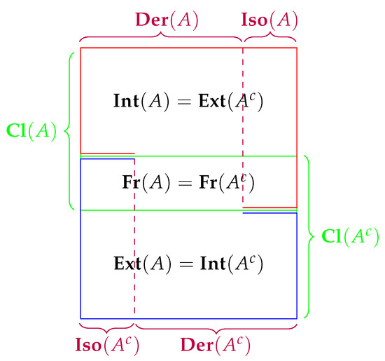
Figure 2. Classifications of Points.

Zarycki [19], in the case of topological space, defined an operator that only captures the portion of boundary (of A) that also belong to A:

$$\mathbf{Br}\left(A\right)\equiv A\cap \mathbf{Fr}\left(A\right).$$

In this way, $\mathbf{Fr}\left(A\right)=\mathbf{Br}\left(A\right)+\mathbf{Br}\left(A^c\right)$, where + stands for “disjoint union”. It was also shown in [19] that this $\mathbf{Br}$ operator can recover the topological space. See discussions in the first paragraph of Section 2. Note that when A is closed iff $\mathbf{Br}\left(A\right)=\mathbf{Fr}\left(A\right)$, while A is open iff $\mathbf{Br}\left(A^c\right)=\mathbf{Fr}\left(A^c\right)$.

In Figure 2, the concept of the derived set is reflected by the portion indicated by the dotted red line and extending all the way to the green line delineating the closure operator. Accumulation points of A (which make up the derived set $\mathbf{Der}\left(A\right)$) can be interior points or boundary points of A, and can belong to A or belong to $A^c$. The operator $\mathbf{Br}$ and $\mathbf{Der}$ are related via

$$\mathbf{Br}\left(A\right)=A\cap \mathbf{Der}\left(A^c\right),\mathbf{Br}\left(A^c\right)=A^c\cap \mathbf{Der}\left(A\right).$$

Although $\mathbf{Br}\left(A\right)$ serves to partition $\mathbf{Fr}\left(A\right)$, $\mathbf{Der}\left(A\right)$ serves to partition $\mathbf{Cl}\left(A\right)$.

We obtain the following two Theorems, which hold for any (generalized) closure systems, instead of topological closure systems.

Theorem 10.

(Partitions of operators).

For any $A\subseteq X$, the following properties hold:

(i)

$\mathbf{Cl}\left(A\right)=\mathbf{Int}\left(A\right)+\mathbf{Fr}\left(A\right)$;

(ii)

$\mathbf{Cl}\left(A\right)=\mathbf{Iso}\left(A\right)+\mathbf{Der}\left(A\right)$;

(iii)

$\mathbf{Cod}\left(A\right)={\left(\mathbf{Der}\left(A^c\right)\right)}^c=\mathbf{Iso}\left(A^c\right)+\mathbf{Int}\left(A\right)$;

(iv)

$X=\mathbf{Int}\left(A\right)+\mathbf{Fr}\left(A\right)+\mathbf{Ext}\left(A\right)$.

Theorem 10 gives two “orthogonal” partitions of $\mathbf{Cl}\left(A\right)$, one involving interior/boundary/ exterior sets, the other involving isolate/derived sets. The former partition describes the “static” relations, while the latter partition describes the “dynamic” relations since a derived set consists of accumulation points in convergence sequences.

We have the following relationship among various types of points.

Theorem 11.

(Relations among operators).

For any $A\subseteq X$, the following properties hold:

(i)

$\mathbf{Cl}\left(A\right)=A\cup \mathbf{Fr}\left(A\right)=A\cup \mathbf{Der}\left(A\right)$;

(ii)

$\mathbf{Cl}\left(A\right)=A\cup (\mathbf{Fr}\left(A\right)\cap \mathbf{Der}\left(A\right))=A\cup (\mathbf{Fr}\left(A\right)\cap A^c)$;

(iii)

$\mathbf{Fr}\left(\mathbf{Cl}\right(A\left)\right)\subseteq \mathbf{Fr}\left(A\right)$ and $\mathbf{Fr}\left(\mathbf{Int}\right(A\left)\right)\subseteq \mathbf{Fr}\left(A\right)$;

(iv)

$\mathbf{Fr}\left(A\right)=\mathbf{Cl}\left(A\right)\cap \mathbf{Cl}\left(A^c\right)$; it is a closed set;

(v)

$(\mathbf{Der}\left(A\right)\cap \mathbf{Der}\left(A^c\right))\subseteq \mathbf{Fr}\left(A\right)=\mathbf{Fr}\left(A^c\right)$;

(vi)

$\mathbf{Iso}\left(A\right)\subseteq A\subseteq \left(\mathbf{Iso}\right(A)\cup \mathbf{Der}(A\left)\right)=\mathbf{Cl}\left(A\right)=\left(\mathbf{Int}\right(A)\cup \mathbf{Fr}(A\left)\right)\supseteq A\supseteq \mathbf{Int}\left(A\right)$.

5. Applications with Examples

5.1. Matroid and Antimatroid

Recall that if X is a finite set and $\mathcal{S}$ is a collection of subsets of X, then the pair $(X,\mathcal{S})$ is called a subset system. Topological system is the most popular example of subset system. Closure system is also a kind of subset system, of which topological system is a special case. Matroid and antimatroids are two special kinds of non-topological closure systems, see Refs. [5,6,7,25].

Definition 24.

A subset system $\mathcal{M}=(X,\mathcal{I})$ is called a matroid if $\mathcal{I}$ satisfies the following three properties:

(i)

$\varnothing \in \mathcal{I}$;

(ii)

$A\in \mathcal{I}$, $B\subseteq A\Rightarrow B\in \mathcal{I}$;

(iii)

$A,B\in \mathcal{I}$, $\left|A\right|>\left|B\right|\Rightarrow \exists x\in A\backslash B$ such that $B\cup \left\{x\right\}\in \mathcal{I}$.

The members in the collection $\mathcal{I}$, which consists of subsets of X, are said to be independent; each member of $\mathcal{I}$ is called an independent set. All other subsets of X are said to be dependent sets. Property (iii) is called an Exchange Axiom. Matroids arise as a generalization to the notion of edges of a graph and to the notion of linear independency of vectors in a vector space.

Definition 25.

A subset system $(X,\mathcal{F})$ is an antimatroid if $\mathcal{F}$ satisfies the following three properties:

(i)

$\varnothing \in \mathcal{F}$;

(ii)

$A\in \mathcal{F}$, $A\ne \varnothing \Rightarrow \exists x\in A$ such that $A\backslash \left\{x\right\}\in \mathcal{F}$;

(iii)

$A,B\in \mathcal{F}$, $A⊈B\Rightarrow \exists x\in A\backslash B$ such that $B\cup \left\{x\right\}\in \mathcal{F}$.

The members in the collection $\mathcal{F}$, which consists of subsets of X, are said to be feasible (subsets of X); all other subsets are said to be infeasible. Note that Property (iii) implies that $\mathcal{F}$ is closed (“stable”) under unions.

5.1.1. Operators on Matroid

Recall that each member of $\mathcal{I}$ of an arbitrary matroid $\mathcal{M}=(X,\mathcal{I})$ is an independent set. A maximally independent set in $\mathcal{M}$ (maximal in the sense that adding an element of X will render the originally independent set dependent) is called a basis of $\mathcal{M}$. A minimal dependent set in $\mathcal{M}$ (minimum in the sense that removal of one of its members will render the originally dependent set independent) is called a circuit of $\mathcal{M}$. The collection $\mathcal{C}$ of all circuits of $\mathcal{M}$ has the following properties:

(i)

$\varnothing \notin \mathcal{C}$;

(ii)

if $C_1,C_2\in \mathcal{C}$ and $C_1\subseteq C_2$, then $C_1=C_2$;

(iii)

For any two distinct $C_1,C_2\in \mathcal{C}$, if $e\in C_1\cap C_2$, then there exists $C_3\in \mathcal{C}$ such that $C_3\subseteq (C_1\cup C_2)\backslash \left\{e\right\}$.

The three properties characterize those collections of sets that may be properly called “circuits system” of a matroid $(X,\mathcal{C})$, i.e., let X be a set and $\mathcal{C}$ be a collection of subsets of X satisfying the above three properties. Let $\mathcal{I}$ be the collection of subsets of X that contain no member of $\mathcal{C}$. Then $(X,\mathcal{I})$ is a matroid with $\mathcal{C}$ as its collection of circuits. The set system $(X,\mathcal{C})$ and $(X,\mathcal{I})$ are two equivalent ways of characterizing the same matroid (in the same way that a Topological System can be equivalently characterized as an open set system, or a system of boundaries, derived sets, etc.).

The concept of circuit is useful for defining various set operators on the matroid (as a special case of Closure System described in Section 3 and Section 4). First, we define a closure operator $\mathbf{Cl}$ as follows: for any $A\subset X$, $\mathbf{Cl}\left(A\right)=A\cup \{x\mid \mathcal{M}$ has a circuit C such that $x\in C\subseteq A\cup \left\{x\right\}\}$. A set whose closure equals itself is said to be a closed set—in matroid theory, it is called a flat or a subspace of a matroid. All flats of a matroid, partially ordered by inclusion, form the so-called matroid lattice.

We can have the following two characterizations of the “isolated set” in a matroid $\mathcal{M}$.

Proposition 14.

For an arbitrary matroid $\mathcal{M}=(X,\mathcal{I})$ with $\mathcal{C}$ as its circuit system, the following statements hold.

• Removal any point from a circuit turns the circuit into an isolated set, i.e., given any circuit $C\in \mathcal{C}$, removal of any point for any $x\in C$, $C\backslash \left\{x\right\}$ is an isolated set, i.e., $\mathbf{Iso}(C\backslash \{x\left\}\right)=C\backslash \left\{x\right\}$;
• A set is isolated if and only if it is independent. That it, a set $A\subset X$ is an isolated set in $\mathcal{M}$ if and only if A is independent.

The above two propositions indicates that for matroid, the notion of “isolated set” and the notion of “independent set” coincide. Since isolated point and accumulation point are used in describing convergent sequences, we can say that every point in an independence set is the isolated point of that independent set, while every point of a circuit is the accumulation point of that circuit.

The last statement can also be seen by constructing the derive set operator $\mathbf{Der}$ from the $\mathbf{Cl}$ of a matroid according to Theorem 5:

Proposition 15.

If C is a circuit of a matroid $\mathcal{M}$, then $C\subseteq \mathbf{Der}\left(C\right)$.

5.1.2. Example: Fano Plane

Let $\Pi =(X,\mathcal{L})$ where $X=\{1,2,3,4,5,6,7\}$ and $\mathcal{L}=\{l_1,l_2,l_3,l_4,l_5,l_6,l_7\}$, $l_1=\{1,2,3\}$, $l_2=\{1,4,5\}$, $l_3=\{1,6,7\}$, $l_4=\{2,4,6\}$, $l_5=\{2,5,7\}$, $l_6=\{3,4,7\}$ and $l_7=\{3,5,6\}$. Then $\Pi$ is what is known as the Fano plane (Figure 3).

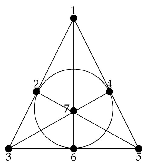
Figure 3. Fano Plane.

Now we can derive the Fano matroid from the Fano plane, a finite geometry with seven points (the seven elements of the matroid) and seven lines (the non-trivial flats of the matroid). We only need to give maximal independent sets: all three-point sets where three points are not collinear, for example, $\{1,2,4\}$. The Fano matroid is a rank-three matroid.

For the Fano matroid, we consider two independent sets: $\{1,2\}$ and $\{1,2,4\}$ as examples. The closures of the two sets: $\mathbf{Cl}\left(\right\{1,2\left\}\right)=\{1,2,3\}$; $\mathbf{Cl}\left(\right\{1,2,4\left\}\right)=\{1,2,3,4,5,6,7\}$. How to describe or classify the points in the two flats $\{1,2,3\}$ and $\{1,2,3,4,5,6,7\}$?

We use two ways to classify the points in a flat, i.e., using two different partitions, $\mathbf{Cl}\left(A\right)=\mathbf{Int}\left(A\right)\cup \mathbf{Fr}\left(A\right)$ and $\mathbf{Cl}\left(A\right)=\mathbf{Iso}\left(A\right)\cup \mathbf{Der}\left(A\right)$. The results are shown as in Table 1.

Table 1. Classification in the Fano Plane.

A	Cl $\left(\mathit{A}\right)$	Int $\left(\mathit{A}\right)$	Fr $\left(\mathit{A}\right)$	Iso $\left(\mathit{A}\right)$	Der $\left(\mathit{A}\right)$
$\{1,2\}$	$\{1,2,3\}$	∅	$\{1,2,3\}$	$\{1,2\}$	$\left\{3\right\}$
$\{1,2,4\}$	$\{1,2,3,4,5,6,7\}$	∅	$\{1,2,3,4,5,6,7\}$	$\{1,2,4\}$	$\{3,5,6,7\}$

Remark 1.

From this example, it follows that for some matroids, independent sets have no interior point while for other matroids, the boundary of any independent sets and theirs derived set are the same. Such classification reflects intrinsic property of points in a matroid.

5.1.3. Example: Antimatroid

Let $X=\{a,b,c,d\}$ and $\mathcal{F}=\{\varnothing ,\{a\},\{c\},\{a,b\},\{a,c\},\{b,c\},\{a,b,c\},\{a,b,c,d\left\}\right\}$. It is easy to check that the subset system $(E,\mathcal{F})$ is an antimatroid (which may be an example of a learning space, see Section 5.2.2 below).

Let us consider three feasible sets: $\left\{a\right\}$, $\{a,b\}$ and $\{a,b,c\}$. Their corresponding classification is shown in Table 2.

Table 2. Classification Results in an Antimatroid.

A	Cl $\left(\mathit{A}\right)$	Int $\left(\mathit{A}\right)$	Fr $\left(\mathit{A}\right)$	Iso $\left(\mathit{A}\right)$	Der $\left(\mathit{A}\right)$
$\left\{a\right\}$	$\{a,d\}$	$\left\{a\right\}$	$\left\{d\right\}$	$\left\{a\right\}$	$\left\{d\right\}$
$\{a,b\}$	$\{a,b,d\}$	$\{a,b\}$	$\left\{d\right\}$	$\{a,b\}$	$\left\{d\right\}$
$\{a,b,c\}$	$\{a,b,c,d\}$	$\{a,b,c\}$	$\left\{d\right\}$	$\{a,c\}$	$\{b,d\}$

5.2. Knowledge Space and Learning Space

The theory of Knowledge Space (and recently, Learning Space) is a well-established set-theoretic framework advanced by Jean-Claude Falmagne and Jean-Paul Doignon [4,26], and has been implemented in computerized tutoring systems, such as RATH and ALEKS. A subject-area or domain of knowledge is conceptualized as a set Q of problems (or questions), and a person’s knowledge state in this domain is formalized as the particular subset of problems this person can solve. All possible knowledge states $\mathcal{K}$ along with the set Q constitute a knowledge space. Formally, the pair $(Q,\mathcal{K})$ is a knowledge space if $\mathcal{K}$ is a collection of subsets of Q which is closed (“stable”) under arbitrary union, and the set system $\mathcal{K}$ includes the ground set Q and the empty set ∅; each member of $\mathcal{K}$ is called a knowledge state. Furthermore, a learning space is defined as follows [4]: A learning space $(Q,\mathcal{L})$ consists of a domain Q (which is a finite set) and a collection $\mathcal{L}$ of subsets of Q (including the empty set ∅ and Q) such that:

(i)

Learning Smoothness. For any two states $K,L$ such that $K⊊L$, there exists a finite chain of states $K=K_0⊊K_1\cdots ⊊K_p=L$ s.t. $|K_i\backslash K_{i-1}|=1$ for $1\le i\le p$.

(ii)

Learning Consistency. If $K,L$ are two states satisfying $K⊊L$ and q is an item such that $K\cup \left\{q\right\}$ is a state, then $L\cup \left\{q\right\}$ is also a state.

A learning space is an instance of an antimatroid, which is an example of a feasible (also called “accessible”) system. Its closure operator satisfies the anti-exchange axiom (instead of the Mac Lane-Steinitz exchange axiom for a matroid, which leads to an independence system).

5.2.1. Inner versus Outer Fringes

Motivated by educational applications, Falmagne and Doignon introduced the notion of fringes of a learning space, and defined both inner fringe and outer fringe. Let $(Q,\mathcal{L})$ be a learning space. For any knowledge state $K\in \mathcal{L}$,

(i)

the inner fringe of K is $K^I=\{q\in K\mid K\backslash \left\{q\right\}\in \mathcal{L}\}$;

(ii)

the outer fringe of K is $K^O=\{q\in K^c\mid K\cup \left\{q\right\}\in \mathcal{L}\}$.

In the language of learning theory, the outer fringe spells out the items that the student is ready to learn, and the inner fringe contains all those items signaling the “high points” in a student’s knowledge state [26].

Falmagne and Doignon showed that any knowledge state in a learning space is uniquely determined by the inner fringe and the outer fringe of this knowledge state, in the sense that $\forall K,L\in \mathcal{L}$,

$$K^I=L^I\mathrm{and}{K}^O=L^O\mathrm{if} \mathrm{and} \mathrm{only} \mathrm{if}K=L.$$

Below, we refine the above conclusion of Falmagne and Doignon, and show that the outer fringe alone (but not inner fringe) specifies the knowledge state.

Proposition 16.

Let $(Q,\mathcal{L})$ be a learning space. Then for any $A\in \mathcal{L}$,

• $\mathbf{Iso}\left(A^c\right)=A^O$;
• $\mathbf{Cl}\left(\mathbf{Iso}\left(A^c\right)\right)=A^c$.

Proof. 

To prove (1), we relate outer fringe to the notion of isolate set $\mathbf{Iso}$ introduced earlier. To prove (2), we invoke a well-known proposition is convex geometry (an equivalent notion of learning space). □

By the above proposition, for any $A\in \mathcal{L}$, $A={\left(\mathbf{Cl}\left(A^O\right)\right)}^c$, which means any knowledge state can be uniquely determined by its outer fringe. We can say the outer fringe also determines the inner fringe of this knowledge state. We conclude that $\forall K,L\in \mathcal{L}$,

$$K^O=L^O\mathrm{if} \mathrm{and} \mathrm{only} \mathrm{if}K=L$$

and

$$K^I=L^I\mathrm{if}{K}^O=L^O$$

.

5.2.2. Example: A 4-Element Knowledge Space (4KS)

Let $Q=\{a,b,c,d\}$ and $\mathcal{L}=\{\varnothing ,\{a\},\{c\},\{a,b\},\{a,c\},\{b,c\},\{a,b,c\},\{a,b,c,d\left\}\right\}.$ It is easy to check that the subset system $(Q,\mathcal{L})$ is a learning space. This is the same example as in Section 5.1.3, so the reader is referred to Table 2 for results of applying set operators.

Remark 2.

It is easily seen that element d is a common boundary point of all non-empty feasible sets. If we partition the points according to exterior/interior/boundary semantics on the one hand, and according to accumulation/isolation semantics on the other, then the same closed set $\mathbf{Cl}\left(A\right)$ may have non-identical partitions. After performing these partitionings for all subset A of Q, it turns out that only the case $A=\{a,b,c\}$ yields different partitioning of $\mathbf{Cl}\left(A\right)=\{a,b,c,d\}$:

$$\mathbf{Cl}\left(A\right)=\mathbf{Int}\left(A\right)\cup \mathbf{Fr}\left(A\right)=\{a,b,c\}\cup \left\{d\right\};$$

$$\mathbf{Cl}\left(A\right)=\mathbf{Iso}\left(A\right)\cup \mathbf{Der}\left(A\right)=\{a,c\}\cup \{b,d\}.$$

In this case, b is an interior point of the feasible set A, and is not an isolation point but an accumulation point with respect to A. In addition, if the interior points of a feasible set are the same as its isolation points, then its boundary is the same as the set of its accumulation points. This shows the points in an antimatroid have different characteristics than those in a matroid.

The next example was taken from an example of learning space studied in [4].

5.2.3. Example: A 5-Element Knowledge Space (5KS)

Let $Q=\{a,b,c,d,e\}$ where Q is a simplistic of knowledge space with five atoms labelled a to e taken from topics of elementary probability and combinatorics [4]. There are 12 possible knowledge states, which are contained in the collection

$$\begin{array}{ccc}\hfill \mathcal{L}& =& \{\varnothing ,\{e\},\{c\},\{e,c\},\{e,c,d\},\{e,c,d,a\},\hfill \\ & & \{e,b\},\{e,b,a\},\{e,b,c\},\{e,b,c,d\},\{e,b,c,a\},\{e,c,d,b,a\}\}.\hfill \end{array}$$

It is easy to verify that $(Q,\mathcal{L})$ is a learning space—each knowledge state (feasible set) is “accessible” from another one by adding one item at a time, creating a chain of “accessibility”. See Figure 4. In fact, $\mathcal{L}$ is a lattice under (the partial order of) set inclusion. The corresponding partial order of $\mathcal{L}$ is shown by Figure 5.

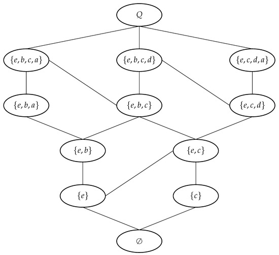
Figure 4. Learning Space $(Q,\mathcal{L})$ with Example 5KS.

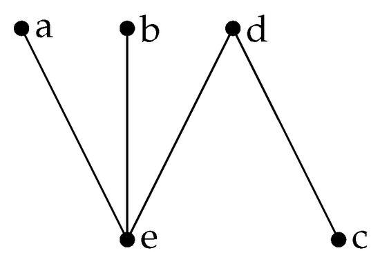
Figure 5. Partial Order Structure of Example 5KS.

We apply the operators to all knowledge states to obtain Table 3.

Table 3. Operations on Knowledge States in 5PS.

A	${\mathit{A}}^{\mathit{c}}$	Iso $\left({\mathit{A}}^{\mathit{c}}\right)$	Cl(Iso(${\mathit{A}}^{\mathit{c}}$))	${\mathit{A}}^{\mathit{O}}$	${\mathit{A}}^{\mathit{I}}$	Fr $\left(\mathit{A}\right)$
∅	Q	$\{e,c\}$	Q	∅	$\{d,a,b\}$	∅
$\left\{c\right\}$	$\{a,b,d,e\}$	$\left\{e\right\}$	$\{a,b,d,e\}$	$\left\{e\right\}$	$\left\{c\right\}$	$\left\{d\right\}$
$\left\{e\right\}$	$\{a,b,c,d\}$	$\{c,b\}$	$\{a,b,c,d\}$	$\{c,b\}$	$\left\{e\right\}$	$\{a,b,d\}$
$\{e,c\}$	$\{a,b,d\}$	$\{b,d\}$	$\{a,b,d\}$	$\{b,d\}$	$\{e,c\}$	$\{d,a,b\}$
$\{e,b\}$	$\{a,c,d\}$	$\{a,c\}$	$\{a,c,d\}$	$\{a,c\}$	$\left\{b\right\}$	$\{a,d\}$
$\{e,b,c\}$	$\{a,d\}$	$\{a,d\}$	$\{a,d\}$	$\{a,d\}$	$\{b,c\}$	$\{a,d\}$
$\{e,b,a\}$	$\{c,d\}$	$\left\{c\right\}$	$\{c,d\}$	$\left\{c\right\}$	$\left\{a\right\}$	$\left\{d\right\}$
$\{e,c,d\}$	$\{a,b\}$	$\{a,b\}$	$\{a,b\}$	$\{a,b\}$	$\left\{d\right\}$	$\{a,b\}$
$\{e,c,d,a\}$	$\left\{b\right\}$	$\left\{b\right\}$	$\left\{b\right\}$	$\left\{b\right\}$	$\left\{a\right\}$	$\left\{b\right\}$
$\{e,b,c,d\}$	$\left\{a\right\}$	$\left\{a\right\}$	$\left\{a\right\}$	$\left\{a\right\}$	$\{d,b\}$	$\left\{a\right\}$
$\{e,b,c,a\}$	$\left\{d\right\}$	$\left\{d\right\}$	$\left\{d\right\}$	$\left\{d\right\}$	$\{c,a\}$	$\left\{d\right\}$
Q	∅	∅	∅	$\{e,c\}$	∅	∅

To demonstrate propositions about inner and outer fringes, let us examine the computation results for three knowledge states $A=\{e,c\},\{e,b,a\},\{e,c,d,a\},$ shown in Table 4. We observe that two different knowledge states $\{e,b,a\}$ and $\{e,c,d,a\}$ have the same inner fringe $\left\{a\right\}$. This is consistent with Proposition 16 that while the outer fringe can uniquely determine a knowledge state, the inner fringe cannot.

Table 4. Selected Knowledge States in Example 5KS.

A	${\mathit{A}}^{\mathit{c}}$	Iso $\left({\mathit{A}}^{\mathit{c}}\right)$	Cl(Iso(${\mathit{A}}^{\mathit{c}}$))	${\mathit{A}}^{\mathit{O}}$	${\mathit{A}}^{\mathit{I}}$	Fr $\left(\mathit{A}\right)$
$\{e,c\}$	$\{a,b,d\}$	$\{b,d\}$	$\{a,b,d\}$	$\{b,d\}$	$\{e,c\}$	$\{d,a,b\}$
$\{e,b,a\}$	$\{c,d\}$	$\left\{c\right\}$	$\{c,d\}$	$\left\{c\right\}$	$\left\{a\right\}$	$\left\{d\right\}$
$\{e,c,d,a\}$	$\left\{b\right\}$	$\left\{b\right\}$	$\left\{b\right\}$	$\left\{b\right\}$	$\left\{a\right\}$	$\left\{b\right\}$

From Table 4, we can compare the difference between the notion of “fringe” and “boundary” of a knowledge state. There is no general relation between the boundary of a knowledge state A and its outer fringe, but inner fringe of A and boundary of A do not intersect: $A^I\cap \mathbf{Fr}\left(A\right)=\varnothing$. The fringe reflects the progression of knowledge acquisition, whereas the boundary reflects the internal logical relations among items.

6. Summary and Conclusions

Our paper advanced the suite of set operators for generalized closure systems—they include, in addition to the closure operator and the dually defined interior operator and exterior operator, a boundary operator, and the dually defined derived-set operator and the co-derived-set operators. The relationships among these six operators are analogous to their relationships in a topological system, so that topological semantics, which are based on the intertwined relations among these operators and their corresponding fixed points, can be extended to the general setting of an arbitrary closure system, including as important examples matroid (independent system) and antimatroid (feasibility system). We showed specifically that contextual classification of points (with respect to a given set) into the several semantic categories follows an identical framework as in topology, which merely enforces an additional axiom regarding finite union or finite intersection (for a closure or interior system, respectively) on top of the three axioms defining a generalized closure/interior system. Therefore, our axiomatization of set operators in closure systems will shed new lights to the interplay of topology, lattice, and logic [11,27]. Our investigations are also significant for axiomatic operators on lattices (posets which are closed with respect to meet and join operations), because closure systems correspond to complete lattices.

We have also cast generalized closure (or interior) systems in the even more general perspective of subset systems. Subset system affords two paths of conceptual development. One, we may treat a subset system simply as a base which can be expanded (through enforcing closure under arbitrary union) to become an interior system. Two, we may rely on the subset system to define accumulation points associated with a converging sequence (through requiring the existence of an additional point as surrogate to the accumulation point during the convergence process) to obtain a system of derived sets. Continuing the path of an interior system (and open sets), we then obtain closure system (and closed sets), from which we develop the notions of boundary points and exterior points. Continuing the path of accumulation points and derived sets, we develop the notions of isolation point and repelling points. The intermediary product of these two paths, namely the interior system induced, and the derived-set system induced from the same subset system, are tightly interlocked and mutually compatible. The semantics of points and set operators under the topological language can be entirely brought over to subset systems. In this way, our results provide a general toolkit with wide potential applicabilities in modern AI systems based on the theory of Knowledge Space/Learning Space, Formal Concept Analysis, Rough Set, etc.

References

- Bourbaki, N. General Topology: Chapters 1–4; Springer Science and Business Media: Berlin/Heidelberg, Germany, 2013; Volume 18. [Google Scholar]
- Dugundji, J. Topology, Series in Advanced Mathematics; Allyn and Bacon, Inc.: Boston, MA, USA, 1966. [Google Scholar]
- Engelking, R. General Topology; PWN-Polish Scientific Publishers: Warszawa, Poland, 1976. [Google Scholar]
- Falmagne, J.-C.; Doignon, J.-P. Learning Spaces; Springer: Berlin, Germany, 2011. [Google Scholar]
- Korte, B.; Lovàsz, L.; Schrader, R. Greedoids; Springer Science and Business Media: Berlin/Heidelberg, Germany, 2012. [Google Scholar]
- Dietrich, B.L. Matroids and antimatroids—A survey. Discret. Math. 1989, 78, 223–237. [Google Scholar] [CrossRef]
- Edelman, P.H.; Jamison, R.E. The theory of convex geometries. Geom. Dedicata 1985, 19, 247–270. [Google Scholar] [CrossRef]
- Ganter, B.; Wille, R. Formal Concept Analysis; Springer: Berlin/Heidelberg, Germany, 1999. [Google Scholar]
- Zhang, G.-Q. Chu Spaces, Concept Lattices, and Domains. Electron. Notes Theor. Comput. Sci. 2003, 83, 287–302. [Google Scholar] [CrossRef][Green Version]
- Barr, M. *-Autonomous Categories, with an Appendix by Po Hsiang Chu. In Lecture Notes in Mathematics 752; Springer: Berlin/Heidelberg, Germany; New York, NY, USA, 1979. [Google Scholar]
- Barr, M. *-Autonomous Categories and Linear Logic. Math. Struct. Comput. Sci. 1991, 1, 159–178. [Google Scholar] [CrossRef]
- Dikranjan, D.; Tholen, W.; Watson, S. Classification of closure operators for categories of topological spaces. In Categorical Structures and Their Applications; Gähler, W., Preuss, G., Eds.; World Scientific: Singapore, 2004; pp. 69–98. [Google Scholar]
- Dikranjan, D.; Giuli, E. Closure operators I. Topol. Appl. 1987, 27, 129–143. [Google Scholar] [CrossRef]
- Gabai, H. The Exterior Operator and Boundary Operator. Am. Math. Mon. 1964, 71, 1029–1031. [Google Scholar] [CrossRef]
- Spira, R. Derived-set axioms for topological spaces. Port. Math. 1967, 26, 165–167. [Google Scholar]
- Steinsvold, C. Topological Models of Belief Logics. Ph.D. Thesis, City University of New York, New York, NY, USA, 2006. [Google Scholar]
- Harvey, F.R. The derived set operator. Am. Math. Mon. 1963, 70, 1085–1086. [Google Scholar] [CrossRef]
- Lei, Y.; Zhang, J. Generalizing topological set operators. In Electronic Notes in Theoretical Computer Science; Elsevier: Amsterdam, The Netherlands, 2019; Volume 345, pp. 63–76. [Google Scholar]
- Zarycki, M. Quelques notions fondamentales de l’Analysis Situs au point de vue de l’Algèbre de la Logique. Fundam. Math. 1927, 9, 3–15, (English translation by Mark Bowron, July 2012). [Google Scholar] [CrossRef][Green Version]
- Melton, A.; Schröder, B.S.; Strecker, G.E. Lagois connections—A counterpart to Galois connections. Theor. Comput. Sci. 1994, 136, 79–107. [Google Scholar] [CrossRef]
- Gediga, G.; Düntsch, I. Modal-style operators in qualitative data analysis. In Proceedings of the IEEE International Conference on Data Mining, Maebashi City, Japan, 9–12 December 2002; pp. 155–162. [Google Scholar]
- Lei, Y.; Luo, M. Rough concept lattices and domains. Ann. Pure Appl. Log. 2009, 159, 333–340. [Google Scholar] [CrossRef]
- Yao, Y.Y. A comparative study of formal concept analysis and rough set theory in data analysis. Lect. Notes Artif. Intell. 2004, 3066, 59–68. [Google Scholar]
- Zhang, J.; Sun, Y. Subset systems: Mathematical abstraction of object and context. In Mathematical Models of Perception and Cognition; Houpt, J., Blaha, L., Eds.; Volume I: A Festschrift for James T. Townsend; Psychological Press, Taylor and Francis (Routledge): New York, NY, USA, 2016; pp. 61–78. [Google Scholar]
- Oxley, J.G. Matroid Theory; Oxford University Press: Oxford, MS, USA, 2006; Volume 3. [Google Scholar]
- Doignon, J.-P.; Falmagne, J.-C. Knowledge Spaces; Springer: Berlin, Germany, 1999. [Google Scholar]
- Davey, B.A.; Priestley, H.A. Introduction to Lattices and Order; Cambridge University Press: Cambridge, UK, 2002. [Google Scholar]
Publisher’s Note: MDPI stays neutral with regard to jurisdictional claims in published maps and institutional affiliations. |
© 2021 by the authors. Licensee MDPI, Basel, Switzerland. This article is an open access article distributed under the terms and conditions of the Creative Commons Attribution (CC BY) license (https://creativecommons.org/licenses/by/4.0/).