Article

Reinitializing Sea Surface Temperature in the Ensemble Intermediate Coupled Model for Improved Forecasts

1
Department of Mathematics, Faculty of Science, King Mongkut’s University of Technology Thonburi, Bangkok 10140, Thailand
2
Department of Mathematics and Statistics, University of Swat, Charbagh 25000, Khyber Pakhtunkhwa, Pakistan
3
Department of Computer Engineering, Biruni University, Istanbul 34010, Turkey
4
Department of Mathematics, Federal University Dutse, Jigawa Gida Sitin, Dutse 720101, Nigeria
*
Author to whom correspondence should be addressed.
Axioms 2021, 10(3), 189; https://doi.org/10.3390/axioms10030189
Submission received: 21 April 2021 / Revised: 7 August 2021 / Accepted: 9 August 2021 / Published: 17 August 2021
(This article belongs to the Special Issue Modern Problems of Mathematical Physics and Their Applications)

Abstract

:
The Ensemble Intermediate Coupled Model (EICM) is a model used for studying the El Niño-Southern Oscillation (ENSO) phenomenon in the Pacific Ocean, which is anomalies in the Sea Surface Temperature (SST) are observed. This research aims to implement Cressman to improve SST forecasts. The simulation considers two cases in this work: the control case and the Cressman initialized case. These cases are simulations using different inputs where the two inputs differ in terms of their resolution and data source. The Cressman method is used to initialize the model with an analysis product based on satellite data and in situ data such as ships, buoys, and Argo floats, with a resolution of 0.25 × 0.25 degrees. The results of this inclusion are the Cressman Initialized Ensemble Intermediate Coupled Model (CIEICM). Forecasting of the sea surface temperature anomalies was conducted using both the EICM and the CIEICM. The results show that the calculation of SST field from the CIEICM was more accurate than that from the EICM. The forecast using the CIEICM initialization with the higher-resolution satellite-based analysis at a 6-month lead time improved the root mean square deviation to 0.794 from 0.808 and the correlation coefficient to 0.630 from 0.611, compared the control model that was directly initialized with the low-resolution in-situ-based analysis.
MSC:
37M05; 37N10; 65K05

1. Introduction

The El Niño–Southern Oscillation (ENSO) is used to describe the Sea Surface Temperature Anomaly (SSTA) in the equatorial Pacific Ocean and ocean–atmosphere system fluctuations in the Southern Hemisphere. Scientists now use the term ENSO warm event to describe the phenomenon where the SST in the eastern and central parts of the Pacific region is warmer than normal, while the term ENSO cold event is now used to describe the phenomenon where the SST in the central and eastern parts of the Pacific region is colder than normal. Many countries in the world are affected by these two phenomena, especially countries in the equatorial parts of the Pacific Ocean. The ENSO is also associated with abnormal climatic conditions, leading to droughts in southern Africa and other areas of the Southern Hemisphere, such as Australia; for example, the Australian continent experienced a drought in 1997 as a result of the ENSO phenomenon. At present, the hot weather in Australia is believed to be the cause of forest fires in Victoria and New South Wales. Southeast Asia, comprising Indonesia, the Philippines, Malaysia, Singapore, Brunei, and Papua New Guinea, experienced the greatest incidence of forest fires in 1997–1998. Moreover, other countries in the region, such as Thailand, Laos, Cambodia, and Vietnam, suffered from drought conditions at this time. The ENSO has been identified as the dominant cause of climate variability around the equatorial Pacific Ocean. It connects the air circulation in the atmosphere with the temperature of water flowing into the Pacific Ocean. International research has shown that the ENSO phenomenon affects more than 70% of the global temperature, although it occurs in the Pacific Ocean.
The modelling of ENSO phenomena has improved, in terms of prediction skills, to within a range of 12 months in advance, based on analyses of the relationships between the atmosphere and ocean. Several studies have been conducted to predict ENSO phenomena using different methods [1,2,3,4,5,6]. Studies have reviewed the efficacy of many models, in an attempt to rule out changes related to ENSO phenomena [7]. The Hybrid Oceanic and Atmospheric System Model (HCM) has been studied to explain climate variability in the tropical Pacific Ocean system [8]. An intermediate coupled model (ICM) has been studied and developed with a variety of methods, in order to improve ENSO forecasting results [9]. Scientists in the Institute of Oceanology, Chinese Academy of Sciences, have studied the evolution of the SST in the tropical Pacific Ocean, as predicted using the IOCAS ICM model. A unique feature is how the temperature of the sub-surface water, entrained into the mixed layer, is parameterized [10]. SST data have been used to predict ENSO phenomena, as an essential geophysical variable that can act as a predictor of atmospheric conditions [1]. The simplest model that can be used to predict the ENSO phenomenon is the EICM. The EICM is constructed from an Intermediate Ocean Model (IOM), which seeks to couple the ocean with entrainment temperature, SST, and wind stress in the tropical Pacific Ocean; however, the observation of oceanic data is very difficult, for various reasons [4], and the resulting inaccuracies in the input data result in incorrect ENSO, leading to incorrect assessment of the model status and its predictions [11]. Therefore, it is necessary to find a procedure that can lead to predictions of the model which are in agreement with the observed data. The unstable data problem may not occur if one uses satellite data, as the model grid resolution is lower than that of the satellite data [12]. For the above reason, discovering an optimal method is necessary for improving initial data, to make them consistent with observation data. Hence, the Cressman initialization method may serve as a potential means to provide the initial data in the EICM.
The data assimilation method is a technique of statistical combination that combines the forecasted result with the initial observation data. This technique is used to correct the initial data that are to be fed into the EICM [13,14]. The process of data assimilation between oceanic and atmospheric improved the El Nino forecasts compared to the forecasting result without data assimilation [15]. The Cressman method has been used to correct the SST data when there are difficulties in measuring the temperatures at exact locations and exact times over vast areas, with satellite-measured observations of sea surface temperature from the MODIS Aqua spectroradiometer [16]. The Cressman method may improve results slightly compared to other methods but is suitable for SST, as shown by [16,17]. Artur et al. (2015) uses Cressman, but applies it to satellite-measured sea surface temperature from the MODIS Aqua spectroradiometer, using a coupled ecosystem model [16]. This procedure provides more correct input data, which may lead to more accurate forecasts and more reliable predictions [18]. Therefore, this work aims to improve the SSTA prediction of the ENSO phenomenon with EICM, using the Cressman initialization method. The Optimum Interpolation Sea Surface Temperature (OISST) data from the Advanced Very High-Resolution Radiometer (AVHRR) was analyzed through the data assimilation process to be used as an input of EICM.

2. Materials and Methods

2.1. Ensemble Intermediate Coupled Model

The EICM was developed from the ICM, in order to improve ENSO phenomenon forecasting results [13], using a different method to generate initial ensemble members with the Markov stochastic random model. Furthermore, the studies of Evensen [19,20] provided a set of initial conditions for an ICM with 100 members. The EICM consists of three main parts: the IOM, the anomaly model for T e and the wind stress [21]. This model has been used to predict ENSO phenomena in tropical regions of the Pacific Ocean [6,22,23]. The anomaly model for T e has been implemented using the prediction of Hybrid Coupled Model (HCM) simulations [24,25] in ENSO. The EICM framework is shown in Figure 1. Keenlyside and Kleeman [26] developed an IOM model to predict the upper ocean currents near the equator, where the model was based on the Baroclinic Euclidean model [27]. These ocean models are able to simulate the variance in SST over the year in several ways. The role of SST in the ENSO has been widely accepted, especially in the eastern Pacific. The SST variance is regulated by zonal and meridional advection and entrainment processes [28]. Zonal currents play important roles in the calculation of the SST in the central Pacific.
The SST component of the model can be formulated using Equation (1). The features of the model that are different from the traditional EICMs are given special attention, which includes simulating the anomalies in the thermocline depth and defining the sub-surface temperature parameters. This model consists of different horizontally blended layers, which serve as the starting point for the various modifications to the traditional EICM. The vertical diffusivity temperature treatment is analogous to the vertical diffusion of momentum in the non-linear component of the model. The equation for SSTA that is implemented in the SST component is written as follows:
T t = u T ¯ x ( u ¯ + u ) T ¯ x v T ¯ y ( v ¯ + v ) T ¯ y w ¯ + w M w ¯ w w ¯ M ( w ¯ ) T ¯ e T ¯ H w ¯ + w M w ¯ w T ¯ e T ¯ H α T + κ h H h · ( H h T ) + 2 κ v H ( H + H 2 ) ( T e T ) ,
where T and T e are the SSTA and water temperature below the mixed layer, respectively; the mean values of the SSTA and the water temperature below the mixed layer are represented by T ¯ and T ¯ e , respectively; the parameters u , v , and w are the corresponding anomaly fields; u ¯ and v ¯ are the prescribed seasonally varying mean zonal and meridional currents in the mixed layer, respectively, and w ¯ is the prescribed seasonally varying mean entrainment velocity at the base of the mixed layer, which are all obtained from the dynamical ocean model; M ( x ) is the Heaviside step function; α T is the surface heat flux term, which is parameterized as being negatively proportional to the local SST anomalies with the thermal damping coefficient; H is the depth of the mixed layer; H 2 is the depth of the second layer [21]; κ h is the coefficient for horizontal diffusivity; κ v is the coefficient for vertical diffusivity; and h = x , y is the horizontal divergence operator.

2.2. Cressman Scheme

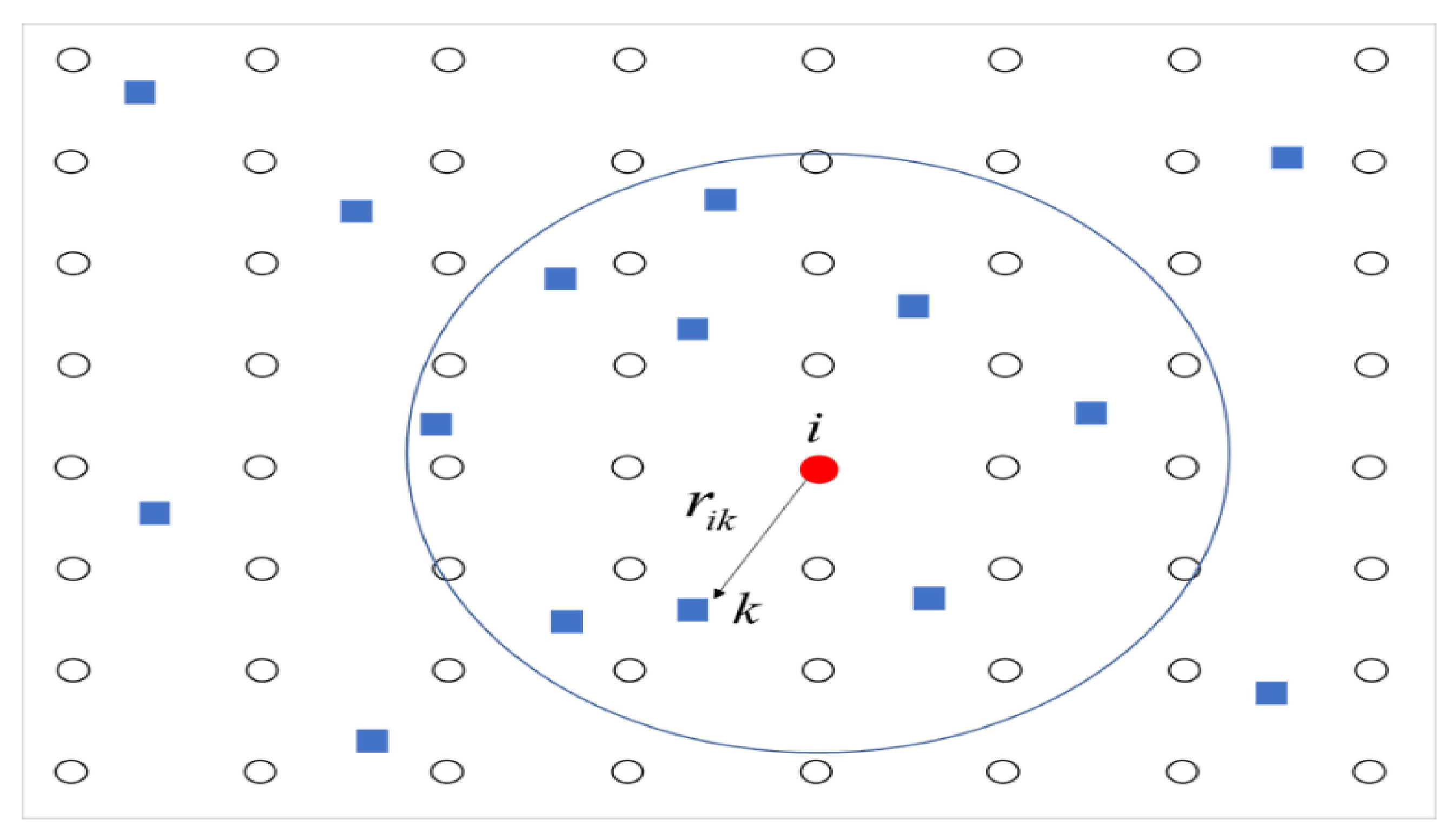
The Cressman technique was developed by George Cressman in 1959, and is the process of modifying the background table point values (derived from the forecast model) by a linear combination of residual values between the predicted and observed values. This technique involves continuously inserting station data into a user-defined latitude–longitude grid, through a grid at a smaller radius of influence, for increased accuracy. The scheme starts with a background field from a numerical forecast, with the background values at each grid point being continuously adjusted based on nearby observations. The advantages of the Cressman method include the associated ease and speed of calculation, combining forecast data into the background field, and offering generally satisfactory results. These multi-faceted advantages of the Cressman method have made it very popular. One disadvantage of the model is that large deviations are often observed around the edges [30]. The Cressman method is not suitable for multiple observations, as it does not take the observational error into account, which is another disadvantage of this method. In this work, the simulation is divided into two cases: the “control” case and the “Cressman initialized” case. Both of these cases are simulations using different inputs where the two inputs differ in terms of their resolution and data source. The control initialized model uses the coarse 2 × 2 degree ICOADS SST data, which provides an analysis that is based solely on in situ data. The Cressman method is used to initialize the model with an analysis product that is based on satellite data AND in situ data, such as ships, buoys, and Argo floats, with a resolution of 0.25 × 0.25 degrees. A schematic of the grid points of the Cressman method is shown in Figure 2.
The model state is assumed to be univariate and is represented as a grid point value. Previous estimates of the model state (background), provided by previous forecasts, are represented by f i n , while observations of the same parameter are represented by f k o , where k = 1 , . . . , K . The Cressman analytical equation is defined by the model state f i n + 1 at each grid point i, according to Equation (2):
f i n + 1 = f i n + k = 1 K w i k n ( f k o f k n ) k = 1 K w i k n + ε 2 ,
where f i n is grid point i of the model at the n th iteration evaluation, f k o is observation point k, f k n is the estimated value at point k of the n th iteration evaluation, ε 2 is the estimation of the error between the model and observed data, and K is the number of observation points. The following equations determine the weights w i k n :
w i k n = R n 2 r i k 2 R n 2 + r i k 2 w h e r e r i k 2 R n 2 0 w h e r e r i k 2 > R n 2 ,
where r i k is the distance between observation point k and grid point i and R n is the radius of the n th iteration evaluation.

2.3. Optimum Interpolation Sea Surface Temperature

NOAA 1/4 daily Optimum Interpolation Sea Surface Temperature (or daily OISST) is an analysis created by combining observations from various platforms, including satellites, boats, buoys, and Argo floats, on a regular global grid. This method includes adjusting the biases of satellite and ship observations (referring to buoys), in order to compensate for platform differences and sensor bias, with a spatially complete SST map being created with corrections to fill the gaps. Satellite data from the Advanced Very High Resolution Radiometer (AVHRR) are the primary input, which have allowed for high temporal and spatial coverage, from late 1981 to the present. The AVHRR is a broadband sensor, featuring three bands in the visible and near-infrared, and three bands in the infrared spectral domain. It is used to represent various world phenomena, in terms of meteorology, soil analysis, and ocean analysis; for example, in the calculation of vegetation indices, cloud properties, dust, snow, ice, fire detection, sea ice concentration, and SST. The spatial resolution of AVHRR is 1 km, at the lowest point reached by a celestial body during its apparent orbit around a given point of observation. These instruments are operated on satellites such as the National Oceanic and Atmospheric Administration (NOAA-11) and European Meteorological Operational (MetOp) satellites. The SST is generated in real-time, using the AVHRR infrared transponder from High-Resolution Picture Transmission (HRPT) using Seaspace’s Tera Scan software and NOAA’s multi-channel regression algorithm [32,33]. The individual SST scenes are daily combined day–night mean grids for the U.S. East coast, where overpasses occur at roughly 1:30 a.m., 9:30 a.m., 1:30 p.m., and 9:30 p.m. (local time) each day. In this work, we considered combining day- and night-time temperatures, in order to represent the daily averaged sea-surface temperature. Daily grids are combined into 3-day, 7-day, monthly, seasonal, and yearly average grids. As this work required monthly SSTA data, NOAA’s daily day–night data were analyzed as monthly data.
The optimum interpolation (OI) sea surface temperature (SST) analysis was performed on a regular grid using irregularly spaced data. The analysis is based on the weighted sum of the data using linear weights OI, which is determined by regression [34].
r k = i = 1 N w i k q i ,
where r k is the analyzed SST, w i k is linear weights, q i are the SST, k is grid points, index i is for data and N is the number of data. The values of q and r are defined as differences from the analysis in the previous time step, and q and r are usually different from the first guess reference system. The average of the analysis correlation error π i π j is assumed to be representative and is proportional of a Gaussian distribution, as follows:
π i π j = e x p ( x i x j ) 2 λ x 2 + ( y i y j ) 2 λ y 2
where π i π j is the average of the analysis correlation error, x and y are the zonal and meridional data and analysis locations, and λ x and λ y are the zonal and meridional spatial scales. The weight was then determined according to Reynolds and Smith 1994 by
i = 1 N π i π j + ϵ i 2 δ i j w i k = π i π j ,
where ϵ i is the noise-to-signal standard deviation ratio, δ i j is data correlation error and w i k is a linear weighting coefficient. The averages of the data errors is assumed to be uncorrelated between the different observations. Therefore, the data correlation error is δ i j = 1 for i = j, and 0 otherwise. Data types currently include ships, buoys, and day and night satellite data for each instrument. Spatial functions are defined for each of these quantities with different ϵ i fields for each data type.

2.4. Extended Reconstructed Sea Surface Temperature

The SSTA data of the National Oceanic and Atmospheric Administration (NOAA, Washington, DC, USA) monthly SST analysis dataset, provided by the Extended Reconstructed Sea Surface Temperature (ERSST) project, were used as input data for the EICM [35,36]. The ERSST dataset is a global monthly SST dataset that derived entirely from in situ observational data and it is provided on a coarse 2 × 2 degree grid, [37,38]. These data were obtained from the International comprehensive Ocean–Atmosphere Dataset (ICOADS) from 1854 until present, as derived from Argo floats above 5 m. The ERSST is suitable for long-term and basin-wide global studies, and uses smooth, specific, and short-term models in the dataset. ERSST version 5 is the newest version of the ERSST, which has improved SST spatial and temporal variability. The newest version of ERSST improves absolute SST, shifting from using the Nighttime Marine Air Temperature (NMAT) to the use of SST buoys as a reference to correct ship SST biases. The ERSST data were used as input to the EICM, as shown in Table 1.
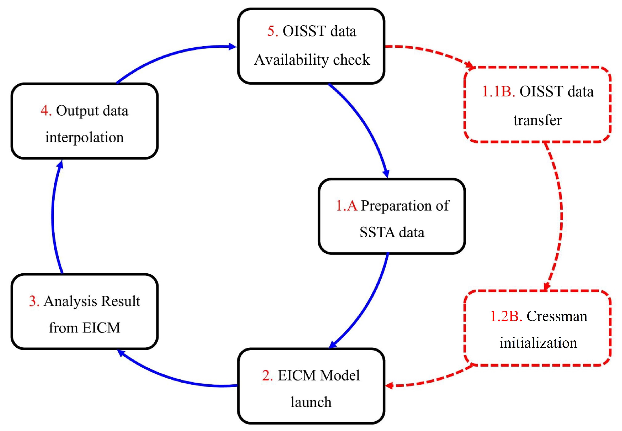
The Cressman analysis procedure was used to improve the accuracy of the model from AVHRR. Subsequently, the system was switched back to the EICM format. Figure 3 shows an outline of how the CIEICM works automatically, using the inputs from the NOAA.

3. Results and Discussion

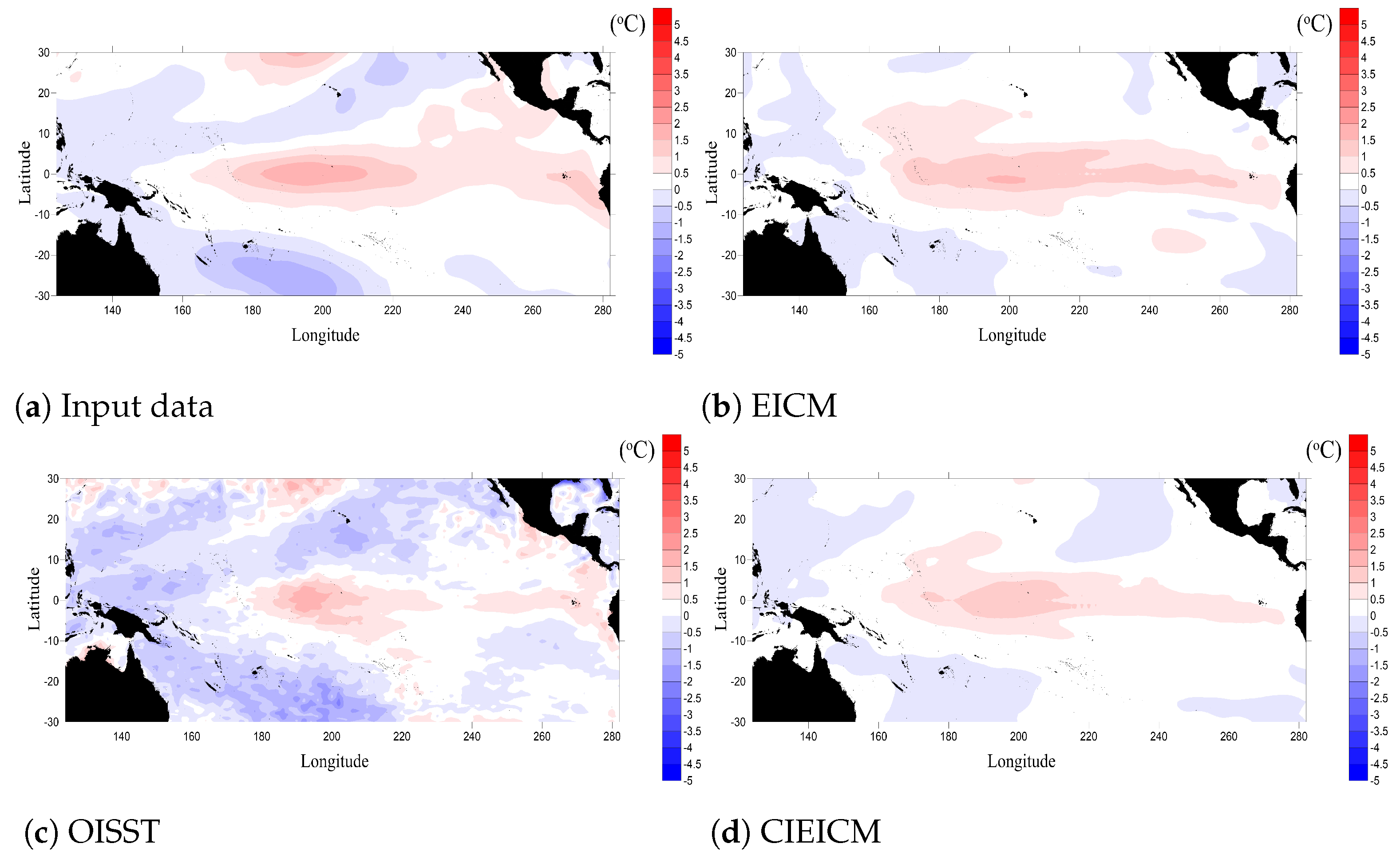
Simulation was performed for the SSTA data of OISST in the EICM and CIEICM, using historical data spanning from 1995 to 2019. The results of EICM and CIEICM simulations were compared with the observed data from NOAA/PMEL TAO buoy network, in order to determine whether the Cressman method had worked properly. A comparison of the SSTA result samples from each simulation with the observations was carried out, in order to assess the accuracy of the preliminary models. The absorption validation with EICM consists of three parts: First, the results of both simulations are compared with the OISST data to determine if the initial method is working correctly. Second, the results of both simulations are compared with source data, to verify the accuracy of the two simulations. Finally, the results of the model are computed, in SSTA index format, in the Niño 3.4 area and compared with data from Hadley Center’s Sea Ice and Sea Surface Temperature (HadISST) [39]. Figure 4 shows the Pacific region SSTA data for January 1995, including SSTA data from ERSST (which was the EICM import data, shown in Figure 4a). The SSTA data of EICM from ICOADS are shown in Figure 4b. The SSTA data, obtained from OISST, are shown in Figure 4c, while SSTA data of CIEICM that Cressman initialized from OISST are shown in Figure 4d.
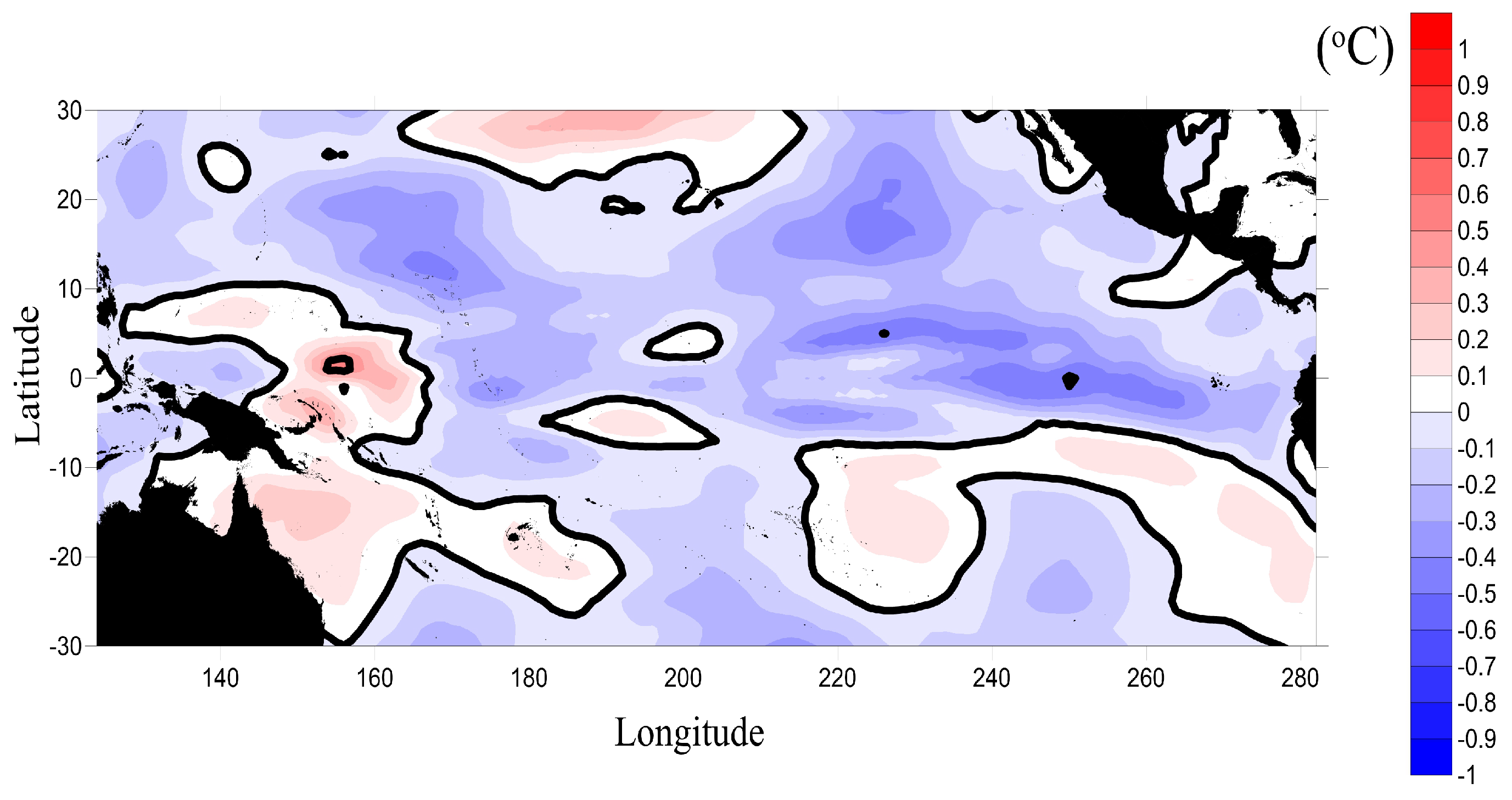
From Figure 4, the OISST data yielded SSTAs lower than those from ERSST and EICM. CIEICM found that most SSTAs were lower than EICM, and similar to those from ERSST and OISST, as expected. Figure 5 shows a comparison of SSTA data from EICM and CIEICM in January 1995, where the blue color means that Cressman Initialized resulted in lower SSTA values. White and red colours indicate that Cressman Initialized increased the SSTA value of the model. The simulation results showed that SSTAs were mostly reduced from EICM, which was consistent with Figure 4.
Visual comparison may not be sufficient and, therefore, a statistical method must be utilised to assess the validity of the model. The statistics used were the Root Mean Square Deviation, shown as Equation (7), Correlation Coefficient, shown as Equation (8), and Standard Deviation of Error, shown in Equation (9).
Root Mean Square Deviation:
R M S D = i = 1 n ( m i o i ) 2 n .
Correlation Coefficient:
R = i = 1 n ( m i m ¯ ) × ( o i o ¯ ) i = 1 n ( m i m ¯ ) 2 × i = 1 n ( o i o ¯ ) 2 .
Standard Deviation:
S D = i = 1 n ( e i e ¯ ) 2 n .
In the above equations, m i denotes the SSTA data from the EICM and CIEICM, o i denotes the SSTA data from OISST, m ¯ denotes the mean SSTA data from EICM and CIEICM, o ¯ denotes the mean SSTA data from OISST, n is the number of grids of data, e i is the Error information between the model and OISST ( m i o i ) , and e ¯ is the mean of the Error. Comparing SSTA data from EICM and CIEICM with the OISST from 1995 to 2019 (i.e., over 25 years), it was found that, when using Cressman Initialized, there was less discrepancy, as the Root Mean Square Deviation value decreased from 0.616 to 0.605. The correlation between the simulation and OISST increased from 0.535 to 0.548, and there was less variation in the error (which decreased from 0.896 to 0.869), as shown in Table 2.
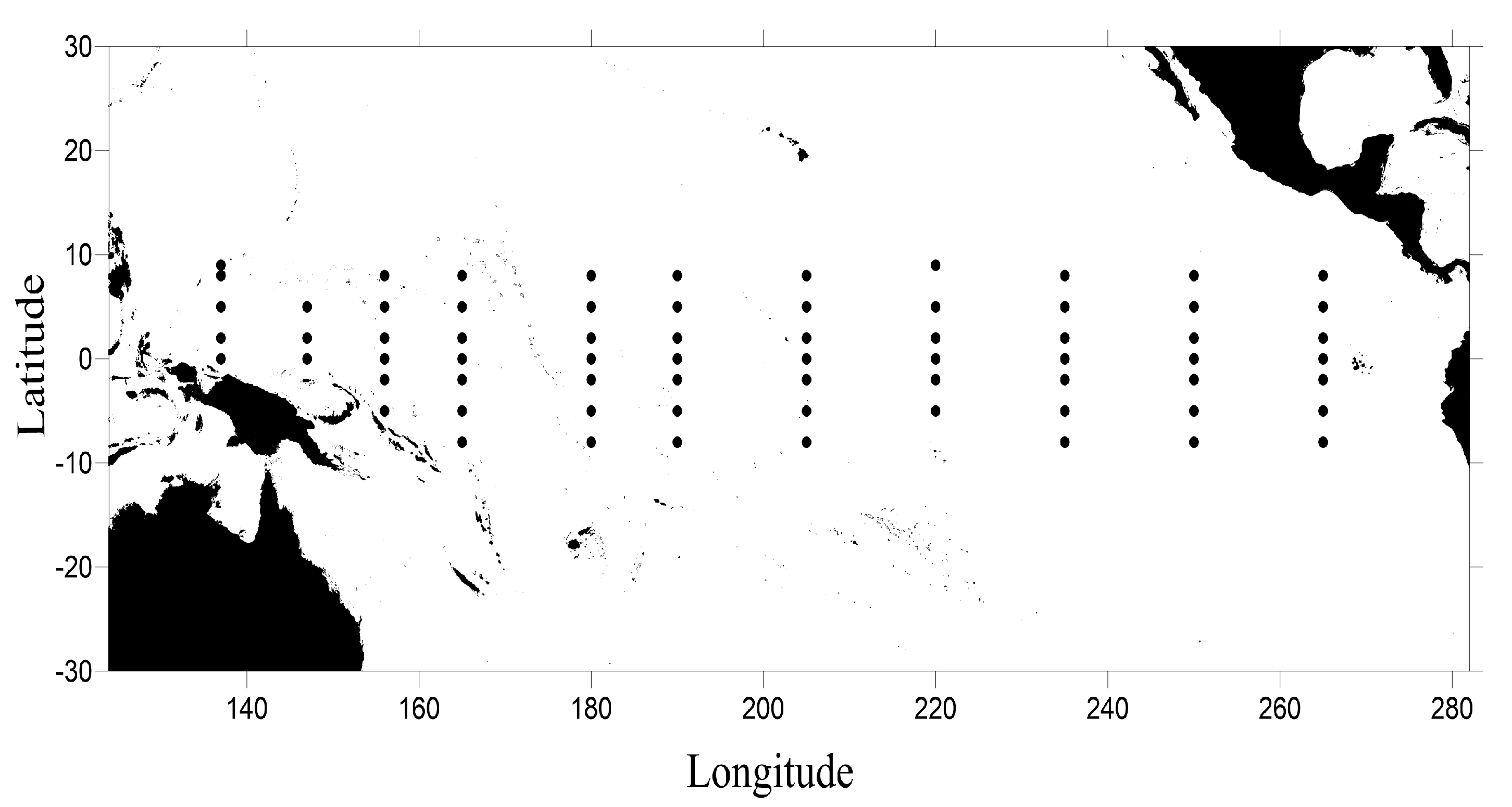
When comparing the CIEICM with OISST, the absorption algorithm worked correctly. A comparison of the precision of both models and OISST with in situ data from 1995 to 2019 was carried out, in order to validate the model and to correlate the model with situational data, where the in situ data were obtained from the NOAA/PMEL TAO buoy network [40,41], for which the buoy locations in the central Pacific Ocean to predict ENSO-related climate variations are shown in Figure 6.
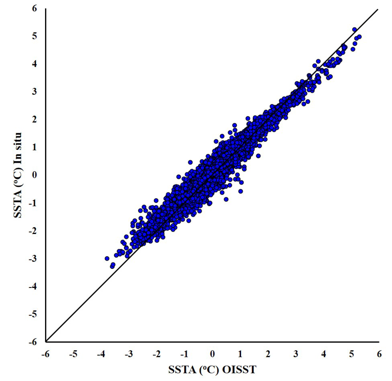
Figure 7 shows the correlation of SSTA data between OISST and source data, with black lines showing that the OISST data and in situ data were highly correlated. If the SSTA value is below the black line, the OISST data were higher than the source data. If the SSTA value is higher than the black line, the OISST data were lower than the source data. From the figure, the data from OISST had a correlation coefficient of 0.968.
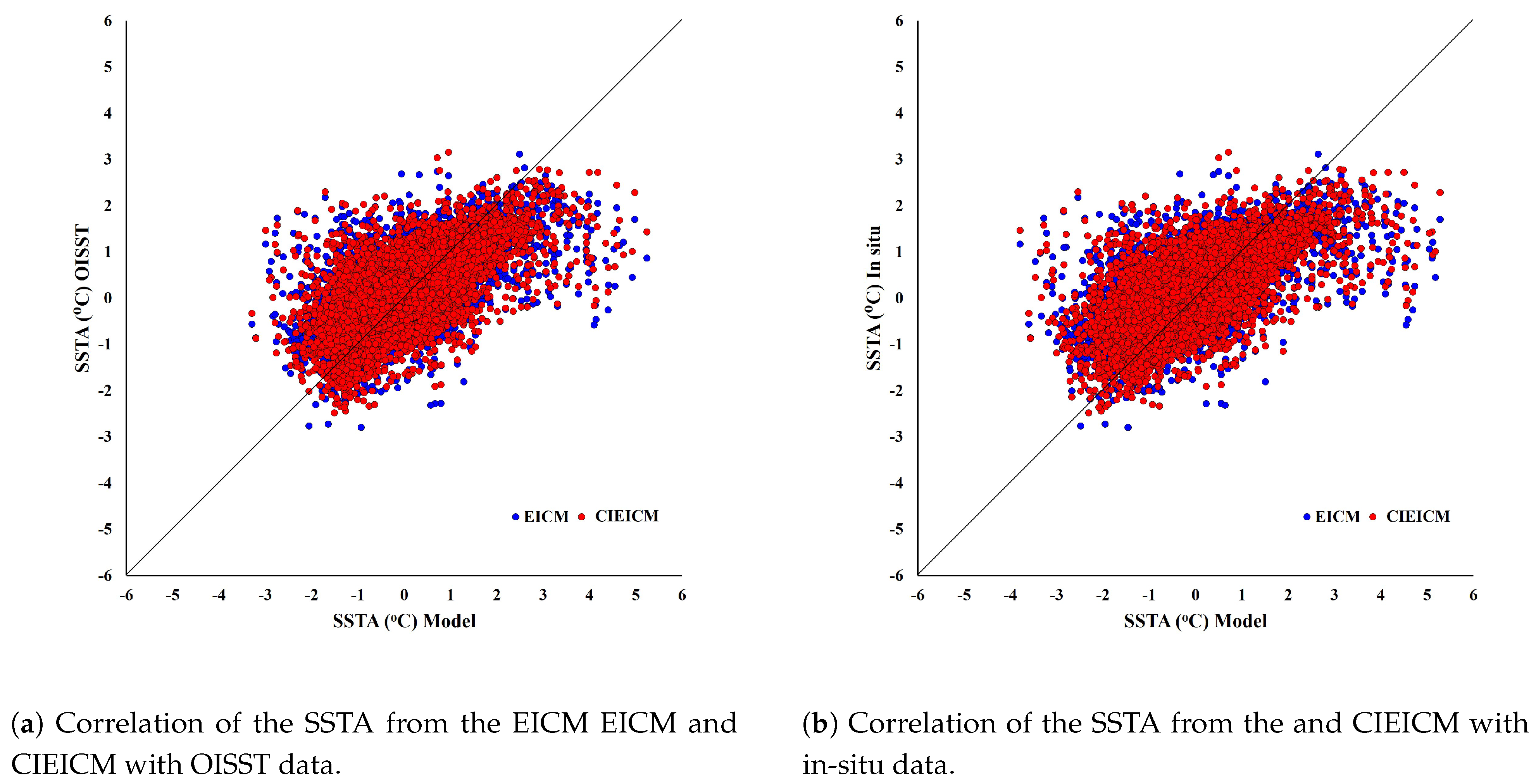
Figure 8a shows the SSTA relationship between EICM or CIEICM and OISST, where blue indicates the relationship between EICM and OISST, and red shows the relationship between CIEICM and OISST. It was found that the EICM was less correlated than that of the CIEICM (at 0.624 and 0.637, respectively). Figure 8b shows the the SSTA relationship between EICM and CIEICM and in situ data, where the blue colour shows the relationship between EICM and in situ data, and red shows the relationship between CIEICM and in situ data. It was found that the EICM was less correlated than that of the CIEICM (at 0.614 and 0.632, respectively).
Comparison of the accuracy of the two simulations with in situ data for each month from 1995 to 2019 found that the CIEICM was able to reduce the model error. During the period from June to August, the model tolerance was better than in other months, where the R M S D from CIEICM was approximately 0.024 less than EICM. When comparing the model relationships, it was found that the CIEICM was more correlated than that of the model; it was also found that the EICM had a correlation of approximately 0.16, as shown in Table 3.
The EICM error was compared with the in situ data, and the CIEICM error was compared with 300 in situ data by the Mann–Whitney U statistical method. Considering the statistical value of the Mann–Whitney U Test, it was found that the value was 41,416.5, and the Asymptotic Significance (1-tailed) value was 0.455, which was compared with the statistical significance level to conclude. As a result of the analysis, the Asymptotic Significance (1-tailed) value was less than the significance level of 0.05. The error from the EICM is greater than the error from the CIEICM, as shown in Table 4.
The Taylor diagram shows a comparison of the SSTA Index in Niño 3.4 (180 E–240 E and 5 S–5 N). The red dot is the SSTA data from the EICM for each ensemble of 100 ensemble and HadISST data. The blue dot is the SSTA data from the CIEICM for each ensemble of 100 ensembles and data from HadISST. The red cross is the SSTA mean from all EICM 100 ensembles and data from HadISST, and the blue cross is the SSTA mean from all CIEICM 100 ensembles and data from HadISST. Figure 9 shows the prediction results for each month. It was found that, in the forecast using imported data from December 1994 to November 2019, the forecast from January 1995 to December 2019 had a forecast period of 1 month. The R M S D of each ensemble was 0.53 to 0.55 and the R M S D of the Mean Ensemble was 0.49 over a 12-month forecast period. Forecasts for December 1995 through December 2019 had an R M S D of each ensemble from 1.2 to 1.4 and a Mean Ensemble R M S D of 0.8. When forecasting SSTA in the near-term, there was little discrepancy, while the longer period SSTA forecast increased the error.
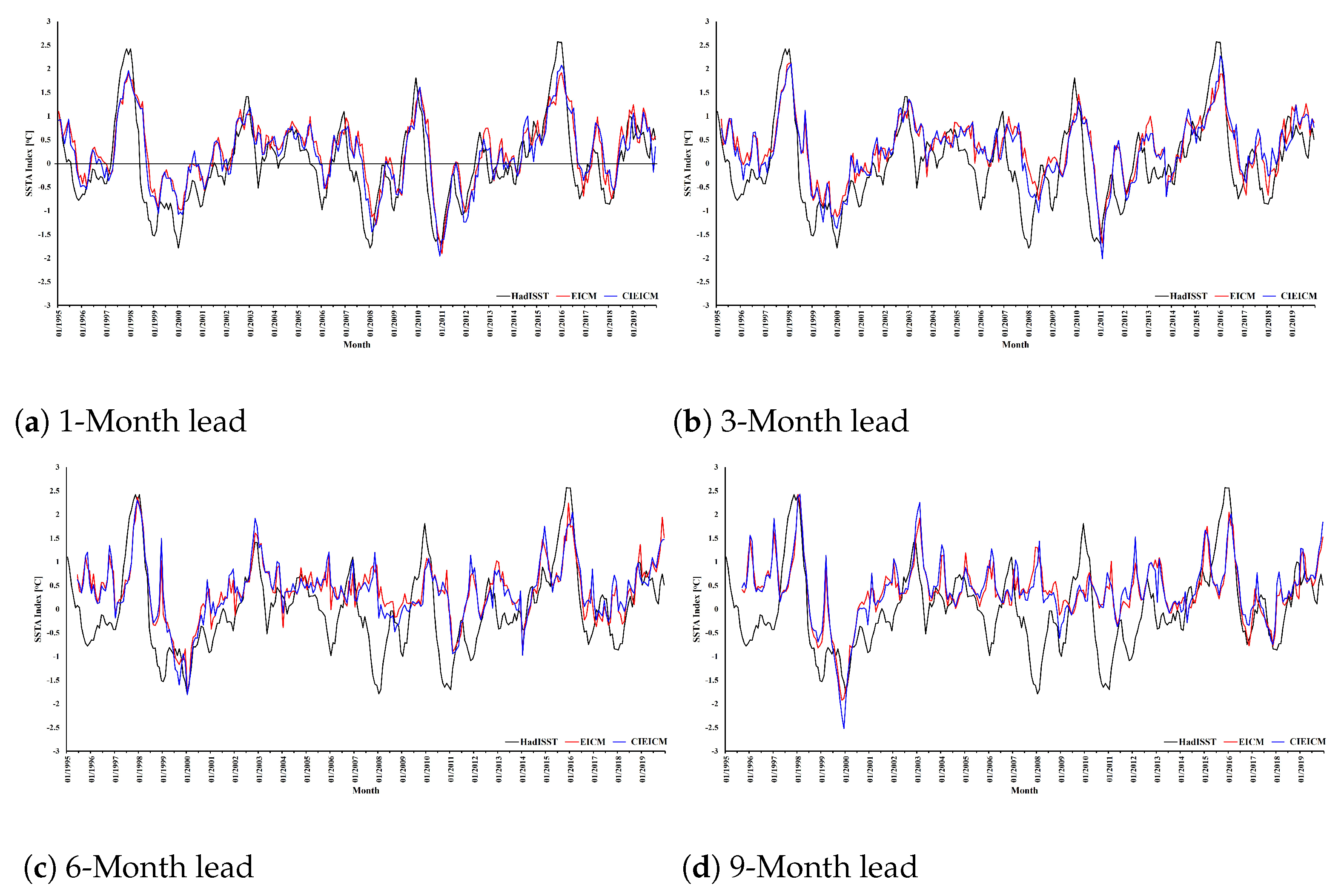
Figure 10 shows the SSTA Index at Niño 3.4, in order to determine the ENSO phenomenon, where the black line is the SSTA Index data from HadISST, the red line is the SSTA Index data from EICM, and the blue line is the SSTA Index data. If the Niño 3.4 index is greater than 0.5, then the El Niño is defined to occur. If the value of the index is between 0.5 and 1, a weak El Niño is defined to occur. If it is between 1 and 1.5, it is defined to be a moderate El Niño. If it is between 1.5 and 2, it is defined to be strong. Finally, if it is greater than 2, it is defined to be very strong. On the other hand, if the Oceanic Niño index is negative and lower than −0.5, then the La Niña is defined to occur. The level of the phenomenon is defined to be divided into weak, moderate, and strong, similar to that for El Niño. The shorter the forecast is, the less accurate the forecast; the longer the forecast, the greater the error.
Comparing the accuracy of the two simulations with HadISST for each month’s lead time from 1995 to 2019, the CIEICM was able to reduce the model error. With 1–8 months lead time, the CIEICM yielded better forecasts than the EICM. With 9–12 months lead time, the two simulations showed no significant differences in terms of R M S D , with the mean R M S D from CIEICM being approximately 0.017 less than EICM. When comparing the model relationships, it was found that the CIEICM was more correlated than the EICM, with an increase of approximately 0.11. In the ranges 1, 2–6, and 7–12 months lead, the relationship was at the levels of very strong, strong, and moderate, respectively, as shown in Table 5.
Figure 11 shows the Pacific SSTA data in November 2015, which includes SSTA data from EICM and SSTA data from CIEICM. It was found that, during the El Niño phenomenon, CIEICM simulations yielded higher SSTAs than EICMs in the Niño region, as shown in Figure 11a,b, respectively. Figure 11c shows the difference between EICM and CIEICM, where blue means that carrying out Cressman Initialized resulted in a decrease in the model’s SSTA, while white and red meant that Cressman Initialization increased the model’s SSTA. Most SSTA values were reduced from EICM.
Figure 12 shows the Pacific SSTA data in January 2000, which includes SSTA data from EICM and SSTA data from CIEICM. It was found that, during the La Niña phenomenon, CIEICM simulation led to lower SSTA than EICM during Niño region, as shown in Figure 12a,b. Figure 12c shows the difference between EICM and CIEICM, where blue means Cressman Initialized decreased the model SSTA, while white and red indicate that Cressman Initialization increased the model SSTA. Most SSTA values were reduced from EICM.

4. Conclusions

Accurately predicting the occurrence of ENSO phenomena several months in advance is a major goal of climate research. It is necessary to find a procedure that can yield model predictions which agree with the observed data. This study, therefore, focused on improving the predictions of ENSO phenomena in the Pacific using the Cressman method to improve SST forecasts with the EICM and CIEICM from 1995 to 2019. The work consisted of three main parts. Part 1, comparing the results from EICM and CIEICM with OISST data, it was found that the Cressman method works properly because the Cressman Initialization method minimizes the error. From the statistical analysis, Root Mean Square Deviation decreased from 0.616 to 0.605, and the relationship between simulation and OISST increased from 0.535 to 0.548. Part 2 compares SST data between EICM that initializing with ICOADS and SST data from NOAA/PMEL TAO buoy network and compares SST data between CIEICM that initializing with Cressman using OISST and SST data from NOAA/PMEL TAO buoy network. It was found that the CIEICM was able to reduce the error each month. The R M S D value decreased from 0.676 to 0.652, and the correlation coefficient increased from 0.600 to 0.616. The results showed that the Asymptotic Significance (1-tailed) value was less than the significance level of 0.05. This means that the test has a greater EICM error than the CIEICM error is shown in Table 4. The last part compared the SSTA index at Niño 3.4 of the two simulations using HadISST data. It was found that the CIEICM was more accurate than the EICM. Moreover, the CIEICM simulation was more correlated with data from HadISST than EICM. Both simulations were able to predict the occurrence of ENSO phenomena well in the first six months, and had a strong correlation. This confirmed the reliability of the algorithm using OISST data in conjunction with the EICM to obtain the CIEICM, which yielded better prediction results.
Several studies have attempted to solve problems associated with the input data used in the model to increase ENSO prediction accuracy. The results of the study of Ji and Leetmaa indicated that adequate physical parameters of data assimilation can improve forecasting results and, thus, improve predictive skills [42]. Chen demonstrated the effects and necessity of data assimilation on ICM and pointed out that assimilation is key in improving the prediction skills of the current ENSO model [43]. Many assimilation techniques have been used for the initial simulation of the ocean atmosphere [44]. A four-dimensional variational (4D-Var) data assimilation method has been implemented in an improved model of the tropical Pacific, in order to improve the accuracy of the model. The results showed that 4D-Var can effectively reduce the error in ENSO analysis [45,46,47]. However, improving forecasting skills by assimilation is not the only method that can be achieved. The need for assimilation may create an imbalance between early ocean conditions and models. The results of the study of Zavala-Garay suggest that there is little room for improvement in predictive skills, as a result of the highly limited data assimilation method [48]. These imbalances and errors in the model can be a significant limiting factor in forecasting skills, especially for predictions that occur in the northern winter. Most studies to date have focused on improving the model through data assimilation, while future studies are expected to focus on optimal error study efforts and actual forecast limit estimates [49]. Some limiting factors cannot be avoided using data assimilation; they have to be addressed through modifications to the model.

Author Contributions

Conceptualization, S.I. and A.K.; methodology, S.I.; software, S.I.; validation, S.I., A.W., U.H. and A.Y.; formal analysis, S.I.; investigation, S.I.; resources, A.W. and A.Y.; data curation, S.I.; writing original draft preparation, S.I.; writing review and editing, S.I.; visualization, A.W. and A.K.; supervision, U.H.; project administration, U.H.; funding acquisition, S.I. All authors have read and agreed to the published version of the manuscript.

Funding

The authors would like to acknowledge the Petchra Pra Jom Klao Ph.D. Research Scholarship from King Mongkut’s University of Technology Thonburi and the authors would like to thank Office of National Higher Education Science Research and Innovation Policy Council [number B16F630087].

Institutional Review Board Statement

Not applicable.

Informed Consent Statement

Not applicable.

Data Availability Statement

Not applicable.

Acknowledgments

The authors would like to thank Office of National Higher Education Science Research and Innovation Policy Council [number B16F630087], Thai Research Fund (TRF) [RDG6230004], and ARDA [PRP6405031190]. The authors would like to acknowledge the Petchra Pra Jom Klao Ph.D. Research Scholarship from King Mongkut’s University of Technology Thonburi.

Conflicts of Interest

The authors declare no conflict of interest.

Abbreviations

The following abbreviations are used in this manuscript:
AVHRRAdvanced Very High-Resolution Radiometer
EICMEnsemble Intermediate Coupled Model
CIEICMCressman Initialized Ensemble Intermediate Coupled Model
ENSOEl Niño–Southern Oscillation
ERSSTExtended Reconstructed Sea Surface Temperature
HadISSTHadley Center’s Sea Ice and Sea Surface Temperature
HCMHybrid Coupled Model
HRPTHigh-Resolution Picture Transmission
ICMIntermediate Coupled Model
IOMIntermediate Ocean Model
MetOpMeteorological Operational
NMATNight-time Marine Air Temperature
NOAANational Oceanic and Atmospheric Administration
OISSTOptimum Interpolation Sea Surface Temperature
RCorrelation Coefficient
R M S D Root Mean Square Deviation
S D Standard Deviation
SSTSea Surface Temperature
SSTASea Surface Temperature Anomaly

References

  1. Merchant, C.J.; Embury, O.; Roberts-Jones, J.; Fiedler, E.; Bulgin, C.; Corlett, G.K.; Good, S.; Mclaren, A.J.; Rayner, N.; Morak-Bozzo, S.; et al. Sea surface temperature datasets for climate applications from Phase 1 of the European Space Agency Climate Change Initiative (SST CCI). Geosci. Data J. 2014, 1, 179–191. [Google Scholar] [CrossRef] [Green Version]
  2. Bjerknes, J. Atmospheric teleconnections from the equatorial Pacific. Mon. Weather Rev. 1969, 97, 163–172. [Google Scholar] [CrossRef]
  3. McCreary, J.P., Jr. A model of tropical ocean-atmosphere interaction. Mon. Weather Rev. 1969, 111, 370–387. [Google Scholar] [CrossRef] [Green Version]
  4. Wyrtki, K. El Niño-the dynamic response of the equatorial Pacific Ocean to atmospheric forcing. J. Phys. Oceanogr. 1975, 5, 572–584. [Google Scholar] [CrossRef]
  5. Cane, M.A.; Zebiak, S.E.; Dolan, S.C. Experimental forecasts of El Niño. Nature 1986, 321, 827–832. [Google Scholar] [CrossRef]
  6. Zhang, R.-H.; Zheng, F.; Zhu, J.; Wang, Z. A successful real-time forecast of the 2010–11 La Niña event. Sci. Rep. 2013, 3, 1–7. [Google Scholar] [CrossRef]
  7. Barnston, A.G.; Tippett, M.K.; L’Heureux, M.L.; Li, S.; DeWitt, D.G. Skill of Real-Time Seasonal ENSO Model Predictions during 2002–11: Is Our Capability Increasing? Bull. Am. Meteorol. Soc. 2012, 93, 631–651. [Google Scholar] [CrossRef]
  8. Barnett, T.P.; Latif, M.; Graham, N.; Flugel, M.; Pazan, S.; White, W. ENSO and ENSO-related predictability. Part I: Prediction of equatorial Pacific sea surface temperature with a hybrid coupled ocean-atmosphere model. J. Clim. 1993, 6, 1545–1566. [Google Scholar] [CrossRef] [Green Version]
  9. Kang, I.S.; Kug, J.S. An El Nino prediction system using an intermediate ocean and a statistical atmosphere. Geophys. Res. Lett. 2000, 27, 1167–1170. [Google Scholar] [CrossRef]
  10. Zhang, R.H.; Gao, C. The IOCAS intermediate coupled model (IOCAS ICM) and its real-time predictions of the 2015-16 El Niño event. Sci. Bull. 2016, 66, 1061–1070. [Google Scholar] [CrossRef] [Green Version]
  11. Zhang, S.; Harrison, M.J.; Wittenberg, A.T.; Rosati, A.; Anderson, J.L.; Balaji, V. Initialization of an ENSO forecast system using a parallelized ensemble filter. Mon. Weather Rev. 2005, 133, 3176–3201. [Google Scholar] [CrossRef]
  12. Webb, D.J.; Cowaed, A.C.; Snaith, H.M. A comparison of ocean model data and satellite observations of features affecting the growth of the North Equatorial Counter Current during the strong 1997–1998 El Niño. Ocean. Sci. 2020, 16, 565–574. [Google Scholar] [CrossRef]
  13. Zheng, F.; Zhang, R.-H. Ensemble hindcasts of SST anomalies in the tropical Pacific using an intermediate coupled model. Geophys. Res. Lett. 2006, 33, 1–5. [Google Scholar] [CrossRef]
  14. Zheng, F.; Zhu, J.; Wang, H.; Zhang, R.-H. Ensemble Hindcasts of ENSO Events over the Past 120 Years Using a Large Number of Ensembles. Adv. Atmos. Sci. 2009, 26, 359–372. [Google Scholar] [CrossRef] [Green Version]
  15. Chen, D.; Zebiak, S.E.; Busalacchi, A.J.; Cane, M.A. An improved procedure for El Niño forecasting: Implications for predictability. Science 1995, 269, 1699–1702. [Google Scholar] [CrossRef] [PubMed] [Green Version]
  16. Artur, N.; Lidia, D.G.; Macigj, J.; Macigi, K. Assimilation of the satellite SST data in the 3D CEMBS model. Oceanologia 2015, 57, 17–24. [Google Scholar]
  17. Abbasi, M.R.; Chegini, V.; Sadrinasab, M.; Siadatmousavi, S.M. Capabilities of data assimilation in correcting sea surface temperature in the Persian Gulf. Pollution 2017, 3, 273–283. [Google Scholar]
  18. Zheng, F.; Zhu, J. Improved ensemble mean forecasting of ENSO events by a zero mean stochastic error model of an intermediate coupled model. Clim. Dyn. 2016, 47, 3901–3915. [Google Scholar] [CrossRef]
  19. Evensen, G. The ensemble Kalman filter: Theoretical formulation and practical implementation. Ocean. Dyn. 2003, 53, 343–367. [Google Scholar] [CrossRef]
  20. Evensen, G. Sampling strategies and square root analysis schemes for the EnKF. Ocean. Dyn. 2003, 54, 539–560. [Google Scholar] [CrossRef]
  21. Zebiak, S.E.; Cane, M.A. A model EI Niño-Southern Oscillation. Mon. Weather Rev. 1987, 115, 2262–2278. [Google Scholar] [CrossRef] [Green Version]
  22. Zhang, R.-H.; Zebiak, S.E.; Kleeman, R. A new intermediate coupled model for El Niño simulation and prediction. Geophys. Res. Lett. 2003, 30, 1–4. [Google Scholar] [CrossRef] [Green Version]
  23. Zhang, R.-H.; Kleeman, R.; Zebiak, S.E.; Keenlyside, N.; Raynaud, S. An empirical parameterization of subsurface entrainment temperature for improved SST simulations in an intermediate ocean model. J. Clim. 2005, 18, 350–371. [Google Scholar] [CrossRef] [Green Version]
  24. Zhu, J.; Zhou, G.; Zhang, R.-H.; Sun, Z. On the role of ocean entrainment temperature (Te) in decadal changes of El Niño/ Southern Oscillation. Ann. Geophys. 2011, 29, 529–540. [Google Scholar] [CrossRef] [Green Version]
  25. Zhu, J.; Zhou, G.; Zhang, R.-H.; Sun, Z. Improving ENSO prediction in a hybrid coupled model with an embedded entrainment temperature parameterization. Int. J. Climatol. 2013, 33, 343–355. [Google Scholar] [CrossRef]
  26. Keenlyside, N.; Kleeman, R. Annual cycle of equatorial zonal currents in the Pacific. Geophys. Res. Lett. 2002, 107, 1–13. [Google Scholar] [CrossRef]
  27. McCreary, J.P. A linear stratified ocean model of the equatorial undercurrent. Philos. Trans. R. Soc. Lond. 1981, 298, 603–635. [Google Scholar]
  28. Gill, A.E. An estimation of sea-level and surface-currents during the 1972 EI Niño and consequenct thermal effects. J. Phys. Oceanogr. 1983, 13, 486–606. [Google Scholar] [CrossRef]
  29. Zhang, R.-H.; Busalacchi, A.J. The Roles of Atmospheric Stochastic Forcing (SF) and Oceanic Entrainment Temperature (Te) in Decadal Modulation of ENSO. J. Clim. 2007, 21, 674–704. [Google Scholar] [CrossRef]
  30. Cressman, G.P. An operational objective analysis system. Mon. Weather Rev. 1959, 87, 367–374. [Google Scholar] [CrossRef]
  31. Kalnay, E. Atmospheric Modeling, Data Assimilation and Predictability; Cambridge University Press: Cambridge, UK, 2003; Volume 87, pp. 136–204. [Google Scholar]
  32. Li, X.; Pichel, W.; Maturi, E.; Clemente-Colon, P.; Sapper, J. Deriving the operational nonlinear multichannel sea surface temperature algorithm coefficients for NOAA-15 AVHRR/3. Int. J. Remote Sens. 2001, 22, 699–704. [Google Scholar] [CrossRef]
  33. Li, X.; Pichel, W.; Clemente-Colon, P.; Krasnopolsky, V.; Sapper, J. Validation of coastal sea and lake surface temperature measurements derived from NOAA/AVHRR data. Int. J. Remote. Sens. 2001, 22, 1285–1303. [Google Scholar] [CrossRef]
  34. Reynolds, R.W.; Smith, T.M. Improved global sea surface temperature analyses. J. Clim. 1994, 7, 929–948. [Google Scholar] [CrossRef] [Green Version]
  35. Smith, T.M.; Reynolds, R.W.; Peterson, T.C.; Lawrimore, J. Improvements NOAAs Historical Merged Land-Ocean Temp Analysis (1880–2006). J. Clim. 2008, 21, 2283–2296. [Google Scholar] [CrossRef]
  36. Xue, Y.; Smith, T.M.; Reynolds, R.W. Interdecadal Changes of 30-Yr SST Normals during 1871–2000. J. Clim. 2003, 16, 1601–1612. [Google Scholar] [CrossRef] [Green Version]
  37. Eric, F.; Elizabeth, C.K.; Philip, B.; Thomas, C.; Lydia, G.; Boyin, H.; Chunying, L.; Shawn, R.S.; Steven, J.W.; Zhang, H.-M. The International Comprehensive Ocean-Atmosphere Data Set— Meeting Users Needs and Future Priorities. Front. Mar. Sci. 2019, 23, 1–8. [Google Scholar]
  38. Liu, W.; Huang, B.; Thorne, P.W.; Banzon, V.F.; Zhang, H.M.; Freeman, E.; Lawrimore, J.; Peterson, T.C.; Smith, T.M.; Woodruff, S.D. Extended Reconstructed Sea Surface Temperature Version 4 (ERSST.v4): Part II. Parametric and Structural Uncertainty Estimations. J. Clim. 2015, 28, 931–951. [Google Scholar] [CrossRef]
  39. Rayner, N.A.; Parker, D.E.; Horton, E.B.; Folland, C.K.; Alexander, L.V.; Rowell, D.P.; Kent, E.C.; Kaplan, A. Global analyses of sea surface temperature, sea ice, and night marine air temperature since the late nineteenth century. J. Geophys. Res. 2003, 108, 4407. [Google Scholar] [CrossRef]
  40. McPhaden, M.J.; Busalacchi, A.J.; Anderson, D.L.T. A TOGA retrospective. Oceanography 2010, 23, 86–103. [Google Scholar] [CrossRef] [Green Version]
  41. McPhaden, M.J.; Busalacchi, A.J.; Cheney, R.; Donguy, J.R.; Gage, K.S.; Halpern, D.; Ji, M.; Julian, P.; Meyers, G.; Mitchum, G.T.; et al. The Tropical Ocean-Global Atmosphere (TOGA) observing system: A decade of progress. J. Geophys. Res. 2020, 103, 14169–14240. [Google Scholar]
  42. Ji, M.; Leetmaa, A. Impact of Data Assimilation on Ocean Initialization and El Niño Prediction. Mon. Weather Rev. 1997, 125, 742–753. [Google Scholar] [CrossRef]
  43. Chen, D. Coupled data assimilation for enso prediction. Adv. Geosci. 2010, 18, 45–62. [Google Scholar]
  44. Oberhuber, J.M. Predicting the E1 Nifio event with a global climate model. Geophys. Res. Lett. 1998, 25, 2273–2276. [Google Scholar] [CrossRef] [Green Version]
  45. Gao, C.; Wu, X.; Zhang, R.H. Testing a Four-Dimensional Variational Data Assimilation Method Using an Improved Intermediate Coupled Model for ENSO Analysis and Prediction. Adv. Atmos. Sci. 2016, 33, 875–888. [Google Scholar] [CrossRef] [Green Version]
  46. Gao, C.; Zhang, R.H.; Wu, X.; Sun, J. Idealized experiments for optimizing model parameters using a 4D-Variational method in an intermediate coupled model of ENSO. Adv. Atmos. Sci. 2018, 35, 410–422. [Google Scholar] [CrossRef]
  47. Injan, S.; Wangwongchai, A.; Humphries, U. Application of Data Assimilation and the Relationship between ENSO and Precipitation. Math. Comput. Appl. 2021, 26, 1–16. [Google Scholar]
  48. Zavala-Garay, J.; Moore, A.M.; Kleeman, R. Influence of stochastic forcing on ENSO prediction. J. Geophys. Res. Ocean. 2004, 109, 1–10. [Google Scholar] [CrossRef]
  49. Tang, Y.; Zhang, R.H.; Liu, T.; Duan, W.; Yang, D.; Zheng, F.; Ren, H.; Lian, T.; Gao, C.; Chen, D.; et al. Progress in ENSO prediction and predictability study. Natl. Sci. Rev. 2018, 5, 826–839. [Google Scholar] [CrossRef]
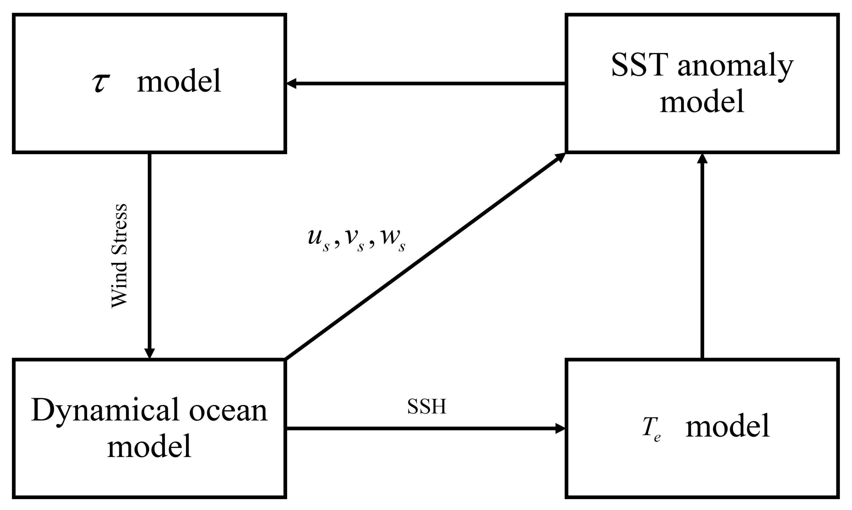
Figure 1. General simple structure of the EICM [29].
Axioms 10 00189 g001
Figure 2. Model data coordinates (circle) and observation data (square) [31].
Axioms 10 00189 g002
Figure 3. CIEICM with the operational assimilation working scheme.
Axioms 10 00189 g003
Figure 4. Comparison of the sample results from the EICM and CIEICM.
Axioms 10 00189 g004
Figure 5. Difference between EICM and CIEICM SSTA data in January 1995.
Axioms 10 00189 g005
Figure 6. Location of measurement data from NOAA/PMEL TAO buoy network.
Axioms 10 00189 g006
Figure 7. Correlation of the SSTA from the OISST with in situ data.
Axioms 10 00189 g007
Figure 8. Correlation of the SSTA from the EICM and CIEICM with OISST and in-situ data.
Axioms 10 00189 g008
Figure 9. Taylor diagram comparing the SSTA index at Niño 3.4 (180 E–240 E and 5 S–5 N).
Axioms 10 00189 g009
Figure 10. ENSO Phenomenon from 1995 to 2019.
Axioms 10 00189 g010
Figure 11. Comparison of the El Niño range.
Axioms 10 00189 g011
Figure 12. Comparison of the El Niño range.
Axioms 10 00189 g012
Table 1. Details of the data in this research.
DetailERSSTOISSTIN SITU
SourceNational Oceanic and Atmospheric Administration (NOAA)
Name of dataSea Surface Temperature Anomaly (SSTA)
Longitude0 E to 360 E0.125 E to 359.875 E137 E to 265 E
Latitude−90 N to 90 N−89.875 N to 89.875 N−8 N to 9 N
Time1854-01 to Present1981-09 to Present1977-01 to Present
Resolution2 × 2 0.25 × 0.25 Point
Searchhttps://www.ncdc.noaa.gov/data-access/marineocean-data/extended-reconstructed-sea-surface-temperature-erssthttps://www.ncdc.noaa.gov/oissthttps://www.pmel.noaa.gov/tao/drupal/disdel/index.html
[accessed on 5 August 2020][accessed on 22 December 2020][accessed on 27 February 2021]
Table 2. Comparison of accuracy between EICM and CIEICM with OISST data.
Model TypeRoot MeanCorrelationStandardSignificance of the Correlation
Square Deviation ( C)Coefficient (−)Deviation ( C)Coefficient (p-Value)
EICM0.6160.5350.8960
CIEICM0.6050.5480.8690
Table 3. Comparison of accuracy between EICM and CIEICM with in situ data.
Month LeadMeasurementsRoot Mean Square DeviationCorrelation Coefficients
EICMCIEICMEICMCIEICM
Jan14130.6910.6690.7770.789
Feb14020.5590.5350.7660.778
Mar14020.5330.5130.6910.718
Apr13910.550.5210.6060.629
May13920.6680.6460.4050.399
Jun13690.7720.7430.3180.336
Jul13830.7740.7440.4360.434
Aug13890.7670.7330.4190.476
Sep13940.7370.710.5160.556
Oct13840.6910.6520.7230.746
Nov13940.6840.6630.7580.763
Dec13960.7100.6650.7700.788
Mean0.6760.6520.6000.616
Table 4. Statistical data analysis results by the Mann–Whitney U Test method.
Mann-Whitney UWilcoxon WZAsymp. Sig (1-Tailed)
R M S D 41,416.586,566.5−1.6880.0455
Table 5. Accuracy comparison between EICM, CIEICM, and HadISST data.
Month LeadMeasurementsRoot Mean Square DeviationCorrelation Coefficients
EICMCIEICMEICMCIEICM
1-Month Lead3000.5550.510.8270.842
2-Month Lead2990.6540.6240.7590.77
3-Month Lead2980.6730.6510.7440.749
4-Month Lead2970.7210.7160.7060.698
5-Month Lead2960.760.7540.6590.676
6-Month Lead2950.8080.7940.6110.63
7-Month Lead2940.8610.8430.550.563
8-Month Lead2930.8970.8770.5060.509
9-Month Lead2920.9040.890.4940.481
10-Month Lead2910.8890.8890.4990.464
11-Month Lead2900.8810.8710.450.499
12-Month Lead2890.8710.8550.4340.489
Mean0.7900.7730.6030.614
Publisher’s Note: MDPI stays neutral with regard to jurisdictional claims in published maps and institutional affiliations.