Abstract
This note is devoted to a robust stability analysis, as well as to the problem of the robust stabilization of a class of continuous-time Markovian jump linear systems subject to block-diagonal stochastic parameter perturbations. The considered parametric uncertainties are of multiplicative white noise type with unknown intensity. In order to effectively address the multi-perturbations case, we use scaling techniques. These techniques allow us to obtain an estimation of the lower bound of the stability radius. A first characterization of a lower bound of the stability radius is obtained in terms of the unique bounded and positive semidefinite solutions of adequately defined parameterized backward Lyapunov differential equations. A second characterization is given in terms of the existence of positive solutions of adequately defined parameterized backward Lyapunov differential inequalities. This second result is then exploited in order to solve a robust control synthesis problem.
Keywords:
Markov jump systems; robust stability; structured parametric uncertainties; stability radius; scaling; linear matrix inequalities MSC:
93E15; 93D09
1. Introduction
The class of Markovian jump linear systems is very appropriate for modeling a plant the structure of which is subject to random abrupt changes. Problems, such as stability and optimal control, as well as important applications of such systems, can be found in several references in the current literature, for instance in [1,2,3,4] and the references therein. On the other hand, robustness, with respect to stochastic parametric uncertainties for this class of system, has attracted a lot of interest from the research community. This is partly due to the engineering applications potential of such a modeling paradigm. We will restrict ourselves in this paper to those works that relied on the concept of stability radii in the treatment of the parametric uncertainties robustness problem. Without being exhaustive, we cite here [5,6,7,8]. For the interested reader, a comprehensive historical perspective of the different aspects regarding the stability radius, both in deterministic and stochastic frameworks, may be found in [9].
In the current paper, we study the robust stability and robust stabilization problems, under multi-perturbations, for a class of continuous-time Markovian jump linear systems affected by parametric uncertainties of multiplicative white noise type with unknown intensity. The only available information is that the intensities of the white noises are output-dependent, unknown, nonlinear functions. In order to effectively address the multi-perturbations case, we will use scaling techniques (see [10,11]) in order to obtain an estimation of the lower bound of the stability radius. We first provide a lower bound of the stability radius in terms of the unique bounded and positive semidefinite solutions of adequately defined parameterized backward Lyapunov differential equations. A second characterization of a lower bound of the stability radius is given in terms of the existence of positive solutions of adequately defined parameterized backward Lyapunov differential inequalities. This second result is very useful for the robust control synthesis problem as it allows the formulation of the feedback gains computation as a convex optimization problem under the Linear Matrix Inequalities (LMIs) paradigm. The original contributions of the paper could be summarized as follows:
- (i)
- An estimation of the lower bound of the stability radius is obtained for a class of continuous-time Markovian jump linear systems subject to block-diagonal stochastic parameter perturbations. The considered parametric uncertainties are of multiplicative white noise type with unknown intensity;
- (ii)
- Scaling techniques have been used in order to effectively address the multi-perturbations case. This allows us to provide a lower bound of the stability radius in terms of the unique bounded and positive semidefinite solutions of adequately defined parameterized backward Lyapunov differential equations;
- (iii)
- A second characterization of a lower bound of the stability radius is given in terms of the existence of positive solutions of adequately defined parameterized backward Lyapunov differential inequalities. This second formulation allows us to state and solve a robust stabilization problem as a convex optimization problem.
Section 2 provides some preliminary definitions and introduces the problem formulation. Several preliminary issues are given in Section 3, which are related to some Lyapunov-type operators as well as to the scaling technique. The main results are established in Section 4. In Section 5, a numerical example is provided to illustrate the theoretical results.
2. Problem Formulation
2.1. Model Description
Let us consider the system , which has the state space representation described by:
, where are state parameters at the instance time t. Here, is an r-dimensional standard Wiener process defined on a given probability space and is a standard Markov process with right-continuous paths and left limits defined on the same probability space , taking values in the finite set and having the transition semigroup , where is a matrix whose elements have the properties:
for all For more details regarding the properties of a standard Wiener process and of the solutions of the stochastic differential equation affected by multiplicative white noise perturbations, we refer to the monographs [12,13,14]. For the properties of the Markov processes, we mention [15,16].
Throughout the paper, we shall write , , , whenever .
Regarding the stochastic processes and the functions that describe the coefficients of the system (1), we make the assumptions:
Hypothesis 1a.
and are -independent stochastic processes;
Hypothesis 1b.
the initial probability distribution of the Markov process , where .
Hypothesis 1c.
, , , , , are bounded and continuous matrix valued functions.
The functions , which model the parametric uncertainties occurring in (1a), satisfy the assumptions:
Hypothesis 2.
The functions are arbitrary nonlinear functions, which are Borel measurable with the property that , , and which satisfy a Lipschitz condition of the form:
, . Throughout the paper, denotes the Euclidean norm of a vector.
The system (1) can be viewed as a disruption of the following system:
which will be named the nominal system. The disruption is produced by a disturbance modeled by the stochastic process:
whose magnitude depends nonlinearly on the output:
Often we shall say that the nominal system is defined by the pair , where are the matrix valued functions satisfying the assumption of Hypothesis 1c and Q is the generator matrix of the Markov process the elements of which satisfy (2).
For each , stands for the -algebra generated by the random variables and with . Further, we denote the set of random vectors , which are -measurable and satisfy . Here, and in the sequel, denotes the mathematical expectation.
Reasoning as in the proof of Theorem 1.1 in Chapter 5 from [12], we obtain the following result regarding the existence of the solution of a stochastic differential equation of type (1) for an arbitrary function , satisfying the assumption of Hypothesis 2.
Proposition 1.
Assume that the matrix valued functions arising in (1) satisfy the assumption Hypotheses 1a–1c. Let and be arbitrary. Then, for any nonlinear function satisfying the assumption Hypothesis 2, the system described by (1) has a unique solution , , which has the properties:
- (a)
- is almost surely continuous in any ;
- (b)
- for any , ;
- (c)
- .
Remark 1.
Since the functions satisfy the assumption of Hypothesis 2, we deduce that the result in Proposition 1 is also applicable in the case of the nominal system (4).
2.2. Robust Stability: Stability Radius
In order to define the concept of robustness of the stability of the zero solution of the nominal system (4) with respect to the structured perturbation (5), we shall introduce a norm in the set of admissible uncertainties of all nonlinear functions of type:
and , and are arbitrary functions satisfying the assumption of Hypothesis 2. To ease the expression of (6), we rewrite it in the form:
where .
We set:
Now we define
where we have denoted
Remark 2.
Among the subsets of the set of admissible uncertainties , we distinguish the subset consisting of all uncertainties of type (6), where
for each , for all , where are arbitrary continuous and bounded matrix valued functions. In this case, the smallest for which the inequality (3) is satisfied is given by:
Let us recall the concept of stability of the zero equilibrium of a system of type (1) and of the nominal system (4) that will be used in the rest of the paper.
Definition 1.
We say that the zero solution of a system , , is:
- (a)
- globally exponentially mean square stable with conditioning (GESMS–C) if there exist , with the property:, , and any initial probability distribution of the Markov process;
- (b)
- globally stochastically stable with conditioning (GSS–C) if there exists with the property:, , and any initial probability distribution of the Markov process.
Remark 3.
- (a)
- (b)
- Since the nominal system (4) is a special case of a system of type (1) (with ), it follows that the previous definition is also applicable in the case of the nominal system. It is worth noting that the system (4) is a linear system and this is why the "global" epithet of the stability is redundant. At the same time, in the linear case, the stability property is not related to a solution, it is a property of the whole system. Therefore, we shall say that the nominal system is exponentially stable in mean square with conditioning (ESMS–C) if its solutions have a behavior like that described by (14).
- (c)
- Applying Theorem 8.3.7 from [4], we deduce that the zero solution of a system is GESMS–C if and only if it is GSS–C.
Roughly speaking, the mean square exponential stability with the conditioning of the nominal system (4) is robust with respect to the structured uncertainties of type (5) if the zero solution of all perturbed systems is ESMS–C for all admissible uncertainties from a subset of .
To measure the level of the robustness of the stability of a linear system of type (4) with respect to the structured uncertainties of type (5) we introduce the following concept of stability radius. This definition is an extension of Definition 3.2 from [18].
Definition 2.
3. Several Preliminary Issues
3.1. The Lyapunov Type Operators and Lyapunov Differential Equations
Let be the linear space of symmetric matrices of size . We set . The elements of are of the form , where , . Equipped with the inner product:
is a finite dimensional ordered Hilbert space. The order relation on denoted by “⪰” is induced by the convex cone . Here, means that is a positive semidefinite matrix.
Based on the coefficients of the nominal system (4), we consider the operator valued function defined by:
, .
Here, denotes the space of the linear operators defined in . In (18b), are the real numbers, which satisfy conditions (2).
.
Let be the linear evolution operator defined by the linear differential equation
that is, , where is the solution of the Lyapunov type differential Equation (20), satisfying .
Applying Theorem 2.7.5 and Theorem 3.2.2 (a) from [4], we obtain:
Proposition 2.
If the nominal system (4) is ESMS–C, then, for each bounded and continuous function , the backward Lyapunov differential equation (BLDE),
has a unique solution which is bounded on . This solution has the representation
Furthermore, if , .
3.2. The Scaling of the Uncertainties
The system (1) may be rewritten into an equivalent form:
where and is defined by
for all .
From (3) and (22), one sees that for any vector of scaling parameters , we have that satisfy the assumption of Hypothesis 2, if satisfy Hypothesis 2.
Moreover, from (8) it follows that
where .
Let us consider the BLDE,
being the operator valued function defined by (19).
Specializing the statement of Proposition 2 to the case of BLDE (25), we obtain:
Proposition 3.
Suppose that the following conditions are satisfied:
- (a)
- The assumption is fulfilled;
- (b)
- The nominal system (4) is ESMS–C;
Under these conditions, for each vector of scaling parameters , , the BLDE (25) has a unique solution which is bounded on and , . Moreover, the dependence with respect to the scaling parameters of the solution is described by
, where for each , is the unique bounded solution of the following BLDE:
4. The Main Results
4.1. A Lower Bound of the Stability Radius
In the sequel, we shall use the notation and the set of the vectors , .
The next Theorem provides a lower bound of the stability radius in terms of the unique bounded and positive semi-definite solutions of the BLDE (25).
Theorem 4.
Assume:
- (a)
- The assumptions and hold true;
- (b)
- The nominal system (4) is ESMS–C.
Let be given. If there exists such that
where is the unique bounded solution of the BLDE (25) associated to the parameter α, then
Proof.
Let be an arbitrary admissible uncertainty satisfying
We show that the corresponding system is GESMS–C. Invoking Proposition 3, we deduce that, under the considered assumptions, the BLDE (25) has a unique bounded on solution , and this solution is positive semidefinite, that is, , .
Applying an Itô type formula (see, for example, Theorem 1.10.2 from [4]) in the case of the function , along the trajectories of the equivalent version (20) of the system , we obtain
, , and is the solution of (1) or, equivalently, of its version (21). Employing (21b) and (25), we rewrite the first integral from the right hand side of (31) as
Setting , we get
, , .
Since is unique bounded on and a positive semi-definite solution of the BLDE (25), we deduce that there exists such that ; This inequality, together with (28) and (34), allow us to infer that:
where does not depend upon .
Letting , we obtain
, , .
, , and does not depend upon , , i.
Applying Theorem 3.6.1 (ii) from [4] in the case of system (1), taking , , , one gets
The next result provides a lower bound of the stability radius of the nominal system (4) with respect to the stochastic structured uncertainties of type (5).
Theorem 5.
Assume that the assumptions of Theorem 4 are fulfilled. Then,
where
being the unique bounded and positive semi-definite solution of the BLDE (25) associated to the vector of scaling parameters .
Proof.
Let us assume by contradiction that (37) is not true. Hence, . Let be such that
Besides BLDE (25), we may consider the following two kinds of backward Lyapunov differential inequalities (BLDIs) on :
and
We recall that if , we shall say that is uniform negative and we shall write , , if there exists such that (i.e., is negative semi-definite), . We will say that is uniform positive on and we shall write , iff is uniform negative on .
Lemma 6.
Under the assumptions Hypotheses 1b and 1c the following hold:
Proof.
□
Now, we provide a lower bound of the stability radius of the nominal system (4) in terms of the solutions of the BLDIs (40) and (41).
Corollary 7.
- (a)
- Assume that the assumptions of Theorem 4 are fulfilled. Let be given. If there exists a vector of scaling parameters and a bounded solution of the corresponding BLDI (40), satisfying the conditionthen
- (b)
- Assume that the assumptions of Hypotheses 1a–1c is fulfilled. If there exists a vector of scaling parameters and a bounded and uniform positive on solution of the BLDI (41) satisfying a condition of type (42), then
- (i)
- the nominal system (4) is ESMS–C;
- (ii)
Proof.
- (a)
- (b)
- The fact that the nominal system is ESMS–C is obtained from Lemma 6 (i). The part (ii) is obtained in the same way as in the proof of (a) from above. Thus the proof ends.
□
4.2. Robust Stabilization via a State Feedback
Let us consider the controlled system,
where are the states of the system at time t and is the vector of the control parameters. If the system (44) is subject to the parametric uncertainties of type (5), it takes the form
. In both (44) and (45) , are bounded and continuous matrix valued functions. The other matrix valued functions involved in (44) and (45) are satisfying the assumptions of Hypotheses 1a–1c and Hypothesis 2.
Our aim is to find conditions that guarantee the existence of a control of type:
which stabilizes the nominal system (44) together with all perturbed systems of type (45), corresponding to the admissible uncertainties satisfying , where is a prescribed level of robustness of the stabilization achieved by the designed control.
An answer to the problem stated here is given in the following theorem:
Theorem 8.
Let be given. Assume:
- (a)
- There exist -matrix valued functions , which are bounded with a bounded derivative;
- (b)
- There exist bounded and continuous matrix valued functions ;
- (c)
- There exist positive scalars , , , , , satisfying the following system of linear matrix inequalities (LMIs):, , , where we denoted, .
Proof.
Pre and post multiplying (47a) by and using the Schur complement technique, we obtain that solves the following BLDI
At the same time, the Schur complement technique used in the case of (47b) allows us to deduce that:
where we have denoted . Rewriting (52) in the equivalent form,
we may obtain, via the definition of the spectral norm of a symmetric and positive semidefinite matrix, that:
for all . The previous inequality yields
where . This allows us to infer that
Remark 4.
- (a)
- It is worth mentioning that if the matrix valued functions, which are involved as coefficients of (47), are periodic functions, and if (47) has a solution and with , , then (47) also has a solution , , which is periodic with the same period as the coefficients of (47);
- (b)
- Since the constant functions can be regarded as periodic functions of an arbitrary period, one obtains that, if the coefficients of (47) do not depend upon t, then (47) has a constant solution and with , if it is solvable. Hence, without loss of generality, in the periodic case to test the solvability of (47) we look for a periodic solution with the same period as the coefficients. Moreover, if the coefficients of (47) do not depend upon t, then we test its solvability, looking for constant solutions.
5. Numerical Experiments
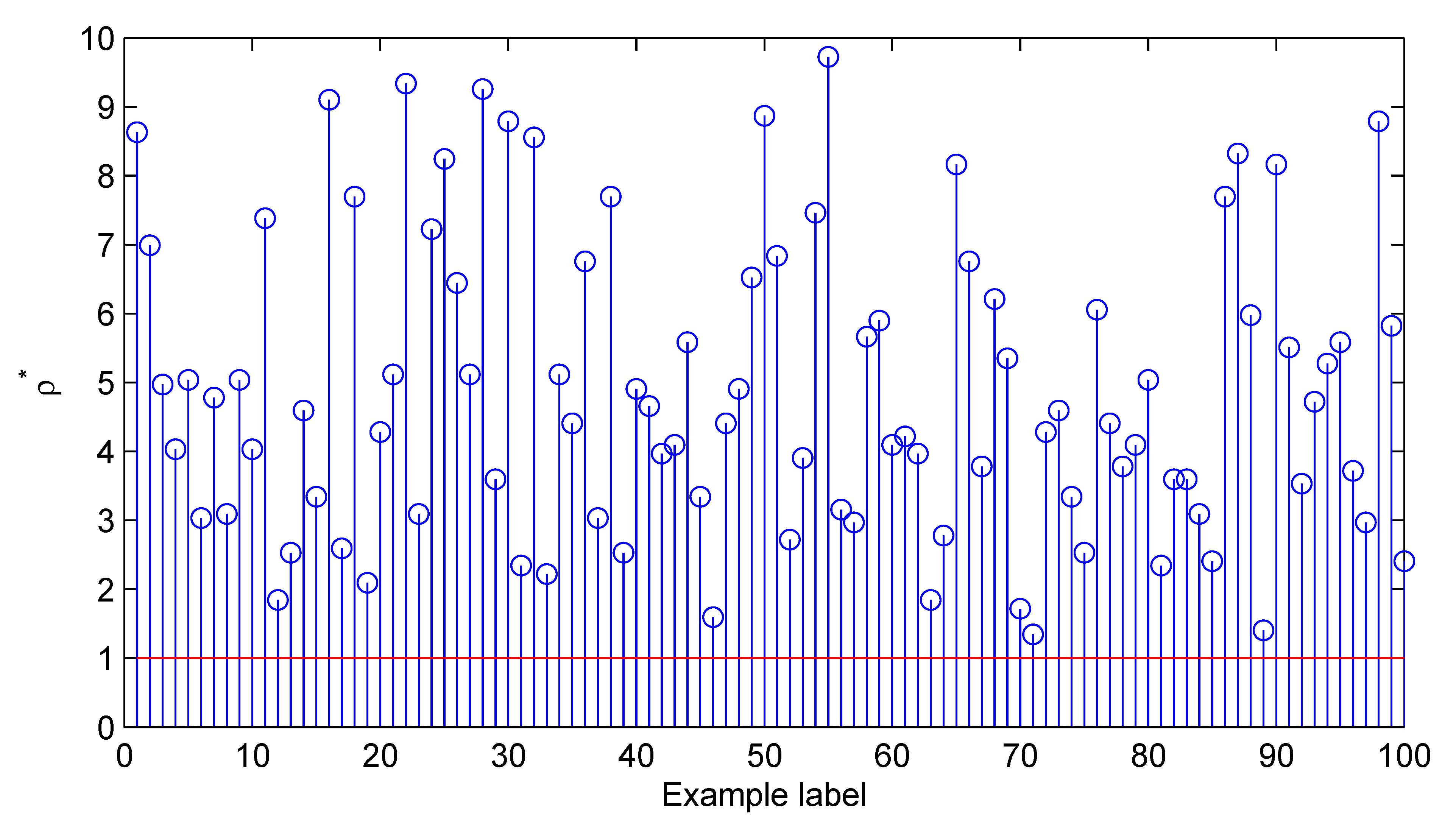
In this section, we will address the problem of robust stabilization described in Section 4.2. We will consider the time-invariant case. This will simplify the presentation and we believe that the conclusions from this section still hold in the time-varying case. The main objective here is to show how the extra degree of freedom provided by the scaling technique allows the improvement of the estimation of the lower bound of the stability radius when compared to a non-scaling one. Let and be the lower bounds corresponding to the non-scaling and the scaling paradigms, respectively. is obtained by solving the following maximization problem under LMIs constraints:
, while is computed using Theorem 8.
We have randomly generated 100 numerical examples and computed for each example the parameter . The obtained results are illustrated by Figure 1. As one expected, one clearly sees the advantage of the scaling technique paradigm.
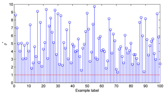
Figure 1.
Plot of the quantity .
6. Conclusions
In this paper, we have addressed the problem of a robust stability analysis of a class of continuous-time Markovian jump linear systems subject to block-diagonal stochastic parameter perturbations. The multi-perturbations case has been efficiently tackled by using scaling techniques. As a robustness metric, we used the concept of stability radius and we obtained an estimation of its lower bound. A first characterization of this lower bound is obtained in terms of solutions of adequately defined parameterized backward Lyapunov differential equations. Then, a second characterization was obtained in terms of solutions of a class of parameterized backward Lyapunov differential inequalities. Based on this result, we solved, in a second step, a state-feedback robust stabilization problem under a convex optimization paradigm.
Our ongoing efforts are devoted, on one hand, to the problem of output–feedback robust stabilization of the considered class of stochastic systems. In this case, only output measurements are available instead of the whole state variables. The resulting robust controller will be in a dynamical/static output–feedback form. Some recent works on the deterministic framework [19,20,21] offer some potential directions to be explored and adapted to our setting. On the other hand, we are interested by the generalization of our results to a more general setting. More specifically, we would like to consider a class of MJLSs with the state space of the underlying Markov chain being countably infinite or being some local compact topological space.
Author Contributions
Conceptualization, V.D. and S.A.; methodology, V.D. and S.A.; software, S.A.; validation, V.D. and S.A.; formal analysis, V.D. and S.A; investigation, V.D. and S.A; writing—original draft preparation, V.D. and S.A.; writing—review and editing, V.D. and S.A. All authors have read and agreed to the published version of the manuscript.
Funding
This research received no external funding.
Institutional Review Board Statement
Not applicable.
Informed Consent Statement
Not applicable.
Data Availability Statement
Not applicable.
Conflicts of Interest
The authors declare no conflict of interest.
References
- Boukas, E.K. Stochastic Switching Systems: Analysis and Design; Birkhauser: Basel, Switzerland, 2004. [Google Scholar]
- Costa, O.L.V.; Fragoso, M.D.; Marques, R.P. Discrete-Time Markov Jump Linear Systems; Springer: Berlin/Heidelberg, Germany, 2005. [Google Scholar]
- Dragan, V.; Morozan, T.; Stoica, A. Mathematical Methods in Robust Control of Discrete-Time Linear Stochastic Systems; Springer: Berlin/Heidelberg, Germany, 2010. [Google Scholar]
- Dragan, V.; Morozan, T.; Stoica, A.M. Mathematical Methods in Robust Control of Linear Stochastic Systems; Springer: New York, NY, USA, 2013. [Google Scholar]
- Aberkane, S.; Dragan, V. Robust Stability and Robust Stabilization of a Class of Discrete-Time Time-Varying Linear Stochastic Systems. SIAM J. Control Optim. 2015, 53, 30–57. [Google Scholar] [CrossRef]
- Dragan, V. Robust stabilization of discrete-time time-varying linear systems with Markovian switching and nonlinear parametric uncertainties. Int. J. Syst. Sci. 2014, 45, 1508–1517. [Google Scholar] [CrossRef]
- El Bouhtouri, A.; Hinrichsen, D.; Pritchard, A.J. Stability radii of discrete-time stochastic systems with respect to blockdiagonal perturbations. Automatica 2000, 36, 1033–1040. [Google Scholar] [CrossRef]
- El Bouhtouri, A.; El Hadri, K. Robust stabilization of discrete-time jump linear systems with multiplicative noise. IMA J. Math. Control Inf. 2005, 23, 447–462. [Google Scholar] [CrossRef]
- Hinrichsen, D.; Pritchard, A.J. Mathematical Systems Theory I, Modeling, State Space Analysis, Stability and Robustness; Springer: Berlin/Heidelberg, Germany, 2005. [Google Scholar]
- Doyle, J. Analysis of feedback systems with structured uncertainties. Proc. IEEE 1986, 129, 242–250. [Google Scholar] [CrossRef] [Green Version]
- Hinrichsen, D.; Pritchard, A.J. Real and complex stability radii: A survey. In Control of Uncertain Systems, Progress in System and Control Theory; Hinrichsen, D., Martensson, B., Eds.; Birkhauser: Basel, Switzerland, 1990; Volume 6, pp. 119–162. [Google Scholar]
- Friedman, A. Stochastic Differential Equations and Applications; Academic: New York, NY, USA, 1975; Volume 1. [Google Scholar]
- Mao, X.; Yuan, C. Stochastic Differential Equations with Markovian Switching; Imperial College Press: London, UK, 2006. [Google Scholar]
- Oksendal, B. Stochastic Differential Equations; Springer: Berlin/Heidelberg, Germany, 1998. [Google Scholar]
- Chung, K.L. Markov Chains with Stationary Transition Probabilities; Springer: Berlin/Heidelberg, Germany, 1967. [Google Scholar]
- Doob, J.L. Stochastic Processes; Wiley: New York, NY, USA, 1967. [Google Scholar]
- Dragan, V.; Morozan, T. Stability and robust stabilization to linear stochastic systems described by differential equations with Markov jumping and multiplicative white noise. Stoch. Anal. Appl. 2002, 20, 33–92. [Google Scholar] [CrossRef]
- Hinrichsen, D.; Pritchard, A.J. Stability radii of systems with stochastic uncertainty and their optimization by output feedback. SIAM J. Control Optim. 1996, 34, 1972–1998. [Google Scholar] [CrossRef] [Green Version]
- Chang, Y.; Zhang, S.; Alotaibi, N.D.; Alkhateeb, A.F. Observer-based adaptive finite-time tracking control for a class of switched nonlinear systems with unmodelled dynamics. IEEE Access 2020, 8, 204782–204790. [Google Scholar] [CrossRef]
- Wang, Y.; Niu, B.; Wang, H.; Alotaibi, N.; Abozinadah, E. Neural network-based adaptive tracking control for switched nonlinear systems with prescribed performance: An average dwell time switching approach. Neurocomputing 2021, 435, 295–306. [Google Scholar] [CrossRef]
- Zhou, P.; Zhang, L.; Zhang, S.; Alkhateeb, A.F. Observer-Based Adaptive Fuzzy Finite-Time Control Design with Prescribed Performance for Switched Pure-Feedback Nonlinear Systems. IEEE Access 2020, 9, 69481–69491. [Google Scholar] [CrossRef]
Publisher’s Note: MDPI stays neutral with regard to jurisdictional claims in published maps and institutional affiliations. |
© 2021 by the authors. Licensee MDPI, Basel, Switzerland. This article is an open access article distributed under the terms and conditions of the Creative Commons Attribution (CC BY) license (https://creativecommons.org/licenses/by/4.0/).