Symmetry Breaking of a Time-2D Space Fractional Wave Equation in a Complex Domain

Abstract

(1) Background: symmetry breaking (self-organized transformation of symmetric stats) is a global phenomenon that arises in an extensive diversity of essentially symmetric physical structures. We investigate the symmetry breaking of time-2D space fractional wave equation in a complex domain; (2) Methods: a fractional differential operator is used together with a symmetric operator to define a new fractional symmetric operator. Then by applying the new operator, we formulate a generalized time-2D space fractional wave equation. We shall utilize the two concepts: subordination and majorization to present our results; (3) Results: we obtain different formulas of analytic solutions using the geometric analysis. The solution suggests univalent (1-1) in the open unit disk. Moreover, under certain conditions, it was starlike and dominated by a chaotic function type sine. In addition, the authors formulated a fractional time wave equation by using the Atangana–Baleanu fractional operators in terms of the Riemann–Liouville and Caputo derivatives.

1. Introduction

Symmetry breaking is a phenomenon in which (infinitesimally) small fluctuations performing on a system possessing a critical point (fixed point, the roots of the transform operator) adopts the system’s outcome, by defining which division of a bifurcation is occupied. This procedure is known symmetry breaking, because such changes typically transform the system from a symmetric but the disorganized state into one or more certain conditions. Symmetry breaking is studied theoretically in the nonlinear optics, lasers, liquid crystals and other areas in physics (see [1,2,3]).

Recently, Sa et al. [4] presented a review study on a complex-plane generalization of the successive distribution utilized to distinguish regular from chaotic quantum spectra. The approach structures the spreading of complex valued ratios between nearest- and next-to-nearest-neighbor spacing. Some results are discussed in the open unit disk.

In this study, we propose a time-2D space fractional wave equation of a complex variable using the modified Atangana–Baleanu fractional differential operator without singular kernel, which is catting in a special class of normalized analytic functions in the open unit disk. Some of its properties are discussed geometrically. The fractional differential operator is used together with a symmetric operator to define a new fractional symmetric operator. Then the new operator is employed to formulate a generalized time-2D space fractional wave equation. Our method is based on the subordination and majorization theory in the open unit disk [5,6]. For two analytic functions f and g in the open unit disk $\mathbb{U}=\{z\in \mathbb{C}:|z|<1\},$ we say that f is majorized by $g(f\ll g)$ if there is an analytic function in the open unit disk $\varpi$ such that $f\left(z\right)=\varpi \left(z\right)g\left(z\right).$ Moreover, f is subordinated to g$(f\prec g)$ if $f\left(z\right)=g\left(\varpi \right(z\left)\right)$ (see [5]). As a result, we obtain altered formulas of analytic geometric solutions based on the geometric function theory.

2. Materials and Methods

Our methods are divided into two subsections as follows:

2.1. Complex Fractional Differential Operator

Fernandez [7] formulated Atangana–Baleanu complex fractional differential operator in terms of the Caputo derivative and the Riemann–Liouville formula respectively, as follows:

$${}^C{\Delta }^{\nu }h\left(z\right)={\displaystyle \frac{\beta \left(\nu \right)}{2\pi i(1-\nu )}}{\int }_{\mathbb{D}}{h}^{\prime }\left(\zeta \right){\mathsf{\Xi }}_{\nu }(-{\mu }_{\nu }{(z-\zeta )}^{\nu })d\zeta ,$$

(1)

where $\beta \left(\nu \right)$ is normalized function by $\beta \left(0\right)=\beta \left(1\right)=1$ and ${\mathsf{\Xi }}_{\nu }\left(w\right)$ is the Mittag–Leffler function

$${\displaystyle {\mathsf{\Xi }}_{\nu }\left(w\right)=\sum _{n=0}^{\infty }\frac{w^n}{\mathsf{\Gamma }(\nu n+1)}.}$$

Moreover, Fernandez [7] introduced the following fractional differential operator

$${}^R{\Delta }^{\nu }h\left(z\right)={\displaystyle \frac{\beta \left(\nu \right)}{2\pi i(1-\nu )}}{\displaystyle \frac{d}{dz}}{\int }_{\mathbb{D}}h\left(\zeta \right){\mathsf{\Xi }}_{\nu }(-{\mu }_{\nu }{(z-\zeta )}^{\nu })d\zeta ,$$

(2)

$$\left({\mu }_{\nu }={\displaystyle \frac{\nu }{1-\nu }},\nu \in [0,1],\mathbb{D}=\{z+r{e}^{i\pi }(z-\ell ):0<r<1\}\right).$$

where ${}^C{\Delta }^{\nu }h\left(z\right)$ is the complex Atangana and Baleanu differential operator in Caputo formula and ${}^R{\Delta }^{\nu }h\left(z\right)$ is the complex Atangana and Baleanu differential operator in the Riemann–Liouville formula. The Atangana–Baleanu fractional operators are used the generalized Mittag–Leffler function as non-local and non-singular kernel. Therefore, they have ability for practising in physics and computational studies. They are recommended in filtering and information theory.

To modify the above operators, we present a class of analytic functions by

$$f\left(z\right)=z+\sum _{n=2}^{\infty }{a}_n{z}^n,z\in \mathbb{U}.$$

This class is denoted by $\mathsf{\Lambda }$ and knowing as the class of univalent functions which is normalized by $f\left(0\right)=f^{\prime }\left(0\right)-1=0.$

Definition 1.

Let $f\in \mathsf{\Lambda }.$ Then the modified operators of (1) and (2) are formulated by the integrals respectively

$${}^C{\Delta }_z^{\nu }f\left(z\right)={\displaystyle \frac{\beta \left(\nu \right)}{1-\nu }}{\int }_0^z{f}^{\prime }\left(\zeta \right){\mathsf{\Xi }}_{\nu ,\upsilon }(-{\mu }_{\nu }{\zeta }^{\nu }){\mathsf{\Xi }}_{\nu }(-{\mu }_{\nu }{(z-\zeta )}^{\nu })d\zeta ,$$

(3)

and

$${}^R{\Delta }_z^{\nu }f\left(z\right)={\displaystyle \frac{\beta \left(\nu \right)}{1-\nu }}{\displaystyle \frac{d}{dz}}{\int }_0^{z}f\left(\zeta \right){\mathsf{\Xi }}_{\nu ,\upsilon }(-{\mu }_{\nu }{\zeta }^{\nu }){\mathsf{\Xi }}_{\nu }(-{\mu }_{\nu }{(z-\zeta )}^{\nu })d\zeta ,$$

(4)

where υ indicates the power of $z.$

For example, let $f\left(z\right)=z,$ then in virtue of [8]—Theorem 2.4 or [9]—Theorem 11.2, we conclude that

$$\begin{array}{cc}\hfill {}^C{\Delta }_z^{\nu }\left(z\right)& =(\beta \left(\nu \right)/1-\nu ){\int }_0^z{\mathsf{\Xi }}_{\nu }(-{\mu }_{\nu }{\zeta }^{\nu }){\mathsf{\Xi }}_{\nu }(-{\mu }_{\nu }{(z-\zeta )}^{\nu })d\zeta \hfill \\ \hfill & =(\beta \left(\nu \right)/1-\nu )z{\mathsf{\Xi }}_{\nu ,2}^2(-{\mu }_{\nu }{\left(z\right)}^{\nu })\hfill \\ \hfill & =(\beta \left(\nu \right)/1-\nu )z\sum _{k=0}^{\infty }{\displaystyle \frac{{\left(2\right)}_k{z}^k}{k!\mathsf{\Gamma }(k\nu +2)}},{(\wp )}_0=1,{(\wp )}_n=\wp (\wp +1)\dots (\wp +n-1).\hfill \end{array}$$

According to [8], Theorem 2.2, we obtain

$$\begin{array}{cc}\hfill {}^R{\Delta }_z^{\nu }\left(z\right)& =(\beta \left(\nu \right)/1-\nu ){\displaystyle \frac{d}{dz}}{\int }_0^z{\mathsf{\Xi }}_{\nu }(-{\mu }_{\nu }{\zeta }^{\nu }){\mathsf{\Xi }}_{\nu }(-{\mu }_{\nu }{(z-\zeta )}^{\nu })\zeta d\zeta \hfill \\ \hfill & =(\beta \left(\nu \right)/1-\nu ){\left(z^2{\mathsf{\Xi }}_{\nu ,3}^2(-{\mu }_{\nu }{\left(z\right)}^{\nu })\right)}^{\prime }\hfill \\ \hfill & =(\beta \left(\nu \right)/1-\nu )\left(z{\mathsf{\Xi }}_{\nu ,2}^2(-{\mu }_{\nu }{\left(z\right)}^{\nu })\right).\hfill \end{array}$$

Clearly, we have

$${}^C{\Delta }_z^{\nu }\left(z\right)={}^R{\Delta }_z^{\nu }\left(z\right).$$

Generally, we have

$${}^C{\Delta }_z^{\nu }\left(z^n\right)=(\beta \left(\nu \right)/1-\nu )n{z}^n\left({\mathsf{\Xi }}_{\nu ,1+n}^2(-{\mu }_{\nu }{\left(z\right)}^{\nu })\right),n\ge 1,$$

$${}^R{\Delta }_z^{\nu }\left(z^n\right)=(\beta \left(\nu \right)/1-\nu )z^n\left({\mathsf{\Xi }}_{\nu ,1+n}^2(-{\mu }_{\nu }{\left(z\right)}^{\nu })\right).$$

Next, we study some properties of the above operators.

Proposition 1.

Consider the operators (3) and (4) for $f\in \mathsf{\Lambda }$. Then by letting $♭\left(\nu \right):=\left(\beta \right(\nu )/1-\nu ),$ the following relations hold

(A) 

$${}^{\mathfrak{C}}{\Delta }_z^{\nu }f\left(z\right):={\displaystyle \frac{{}^C{\Delta }_z^{\nu }f\left(z\right)}{♭\left(\nu \right){\mathsf{\Xi }}_{\nu ,2}^2(-{\mu }_{\nu }{\left(z\right)}^{\nu })}}\in \mathsf{\Lambda }$$

and

$${}^{\mathfrak{R}}{\Delta }_z^{\nu }f\left(z\right):={\displaystyle \frac{{}^R{\Delta }_z^{\nu }f\left(z\right)}{♭\left(\nu \right){\mathsf{\Xi }}_{\nu ,2}^2(-{\mu }_{\nu }{\left(z\right)}^{\nu })}}\in \mathsf{\Lambda },$$

(B) 

${}^{\mathfrak{R}}{\Delta }_z^{\nu }f\left(z\right)\ll {}^{\mathfrak{C}}{\Delta }_z^{\nu }f\left(z\right),$

(C) 

${}^{\mathfrak{R}}{\Delta }_z^{\nu }f\left(z\right)\prec {}^{\mathfrak{C}}{\Delta }_z^{\nu }f\left(z\right),$ provided that ${}^{\mathfrak{C}}{\Delta }_z^{\nu }f\left(z\right),$ is locally univalent of the first order (like convex function [10]) when $\left|z\right|\in (0.28,\sqrt{2}-1]$ or locally univalent of the second order (like the class of univalent functions [10]) when $\left|z\right|\in (0.21,0.3).$

Proof. 

For $f\in \mathsf{\Lambda },$ a computation brings

$$\begin{array}{cc}\hfill {}^{\mathfrak{C}}{\Delta }_z^{\nu }f\left(z\right)& ={\displaystyle \frac{{}^C{\Delta }_z^{\nu }f\left(z\right)}{♭\left(\nu \right){\mathsf{\Xi }}_{\nu ,2}^2(-{\mu }_{\nu }{\left(z\right)}^{\nu })}}\hfill \\ \hfill & ={\displaystyle \frac{♭\left(\nu \right){\mathsf{\Xi }}_{\nu ,2}^2(-{\mu }_{\nu }{\left(z\right)}^{\nu })z+{\sum }_{n=2}^{\infty }{a}_n♭\left(\nu \right)n\left({\mathsf{\Xi }}_{\nu ,1+n}^2(-{\mu }_{\nu }{\left(z\right)}^{\nu })\right)z^n}{♭\left(\nu \right){\mathsf{\Xi }}_{\nu ,2}^2(-{\mu }_{\nu }{\left(z\right)}^{\nu })}}\hfill \\ \hfill & =z+\sum _{n=2}^{\infty }{a}_{n}n\left({\displaystyle \frac{{\mathsf{\Xi }}_{\nu ,1+n}^2(-{\mu }_{\nu }{\left(z\right)}^{\nu })}{{\mathsf{\Xi }}_{\nu ,2}^2(-{\mu }_{\nu }{\left(z\right)}^{\nu })}}\right)z^n\hfill \\ \hfill & \Rightarrow {}^{\mathfrak{C}}{\Delta }_z^{\nu }f\left(z\right)\in \mathsf{\Lambda }.\hfill \end{array}$$

Similarly, we have ${}^{\mathfrak{R}}{\Delta }_z^{\nu }f\left(z\right)\in \mathsf{\Lambda }.$ This completes the first part. For the second part, it is adequate to show that (see [11])

$${|}^{\mathfrak{R}}{\Delta }_z^{\nu }{f\left(z\right)|\le |}^{\mathfrak{C}}{\Delta }_z^{\nu }f\left(z\right)|.$$

A calculation yields

$$\begin{array}{cc}\hfill {|}^{\mathfrak{R}}{\Delta }_z^{\nu }f\left(z\right)|& =|z+\sum _{n=2}^{\infty }{a}_n\left({\displaystyle \frac{{\mathsf{\Xi }}_{\nu ,1+n}^2(-{\mu }_{\nu }{\left(z\right)}^{\nu })}{{\mathsf{\Xi }}_{\nu ,2}^2(-{\mu }_{\nu }{\left(z\right)}^{\nu })}}\right)z^n|\hfill \\ \hfill & \le |z+\sum _{n=2}^{\infty }{a}_{n}n\left({\displaystyle \frac{{\mathsf{\Xi }}_{\nu ,1+n}^2(-{\mu }_{\nu }{\left(z\right)}^{\nu })}{{\mathsf{\Xi }}_{\nu ,2}^2(-{\mu }_{\nu }{\left(z\right)}^{\nu })}}\right)z^n|\hfill \\ \hfill & {=|}^{\mathfrak{C}}{\Delta }_z^{\nu }f\left(z\right)|.\hfill \end{array}$$

The last part immediately recognizes by [11]—Corollaries 1 and 2 respectively. □

2.2. Symmetric Fractional Differential Operator (SFDO)

For a function $f\left(z\right)\in \mathsf{\Lambda }$ and a constant $ð\in [0,1],$ the SFDO can be defined by using ${}^{\mathfrak{R}}{\Delta }_z^{\nu }f\left(z\right)$ or ${}^{\mathfrak{C}}{\Delta }_z^{\nu }f\left(z\right)$ as follows:

$$\begin{array}{cc}\hfill & {}^{\mathfrak{R}}{\left({\mathcal{S}}_{ð}^{\nu }\right)}^{0}f\left(z\right)=f\left(z\right)\hfill \\ \hfill & {}^{\mathfrak{R}}{\left({\mathcal{S}}_{ð}^{\nu }\right)}^{1}f\left(z\right)=ð\left({}^{\mathfrak{R}}{\Delta }_z^{\nu }f\right)\left(z\right)-(1-ð)\left({}^{\mathfrak{R}}{\Delta }_z^{\nu }f\right)(-z)\hfill \\ \hfill & =ð\left(z+\sum _{n=2}^{\infty }{a}_n\left({\displaystyle \frac{{\mathsf{\Xi }}_{\nu ,1+n}^2(-{\mu }_{\nu }{\left(z\right)}^{\nu })}{{\mathsf{\Xi }}_{\nu ,2}^2(-{\mu }_{\nu }{\left(z\right)}^{\nu })}}\right)z^n\right)\hfill \\ \hfill & -(1-ð)\left(-z+\sum _{n=2}^{\infty }{(-1)}^n{a}_n\left({\displaystyle \frac{{\mathsf{\Xi }}_{\nu ,1+n}^2(-{\mu }_{\nu }{(-z)}^{\nu })}{{\mathsf{\Xi }}_{\nu ,2}^2(-{\mu }_{\nu }{(-z)}^{\nu })}}\right)z^n\right)\hfill \\ \hfill & =z+\sum _{n=2}^{\infty }\left(ð\left({\displaystyle \frac{{\mathsf{\Xi }}_{\nu ,1+n}^2(-{\mu }_{\nu }{\left(z\right)}^{\nu })}{{\mathsf{\Xi }}_{\nu ,2}^2(-{\mu }_{\nu }{\left(z\right)}^{\nu })}}\right)-(1-ð){(-1)}^n\left({\displaystyle \frac{{\mathsf{\Xi }}_{\nu ,1+n}^2(-{\mu }_{\nu }{(-z)}^{\nu })}{{\mathsf{\Xi }}_{\nu ,2}^2(-{\mu }_{\nu }{(-z)}^{\nu })}}\right)\right)a_n{z}^n\hfill \\ \hfill & :=z+\sum _{n=2}^{\infty }{\complement }_n^{\nu ,ð}\left(z\right)a_n{z}^n\hfill \\ \hfill & {}^{\mathfrak{R}}{\left({\mathcal{S}}_{ð}^{\nu }\right)}^{2}f\left(z\right)={}^{\mathfrak{R}}{\left({\mathcal{S}}_{ð}^{\nu }\right)}^1{[}^{\mathfrak{R}}{\left({\mathcal{S}}_{ð}^{\nu }\right)}^{1}f\left(z\right)]=z+\sum _{n=2}^{\infty }{\left[{\complement }_n^{\nu ,ð}\left(z\right)\right]}^2{a}_n{z}^n\hfill \\ \hfill & ⋮\hfill \\ \hfill & {}^{\mathfrak{R}}{\left({\mathcal{S}}_{ð}^{\nu }\right)}^{k}f\left(z\right)={}^{\mathfrak{R}}{\left({\mathcal{S}}_{ð}^{\nu }\right)}^1{[}^{\mathfrak{R}}{\left({\mathcal{S}}_{ð}^{\nu }\right)}^{k-1}f\left(z\right)]=z+\sum _{n=2}^{\infty }{\left[{\complement }_n^{\nu ,ð}\left(z\right)\right]}^k{a}_n{z}^n.\hfill \end{array}$$

(5)

Similarly, we can use ${}^{\mathfrak{C}}{\Delta }_z^{\nu }f\left(z\right)$ to obtain the following SFDO

$${}^{\mathfrak{C}}{\left({\mathcal{S}}_{ð}^{\nu }\right)}^{k}f\left(z\right)={}^{\mathfrak{C}}{\left({\mathcal{S}}_{ð}^{\nu }\right)}^1{[}^{\mathfrak{C}}{\left({\mathcal{S}}_{ð}^{\nu }\right)}^{k-1}f\left(z\right)]=z+\sum _{n=2}^{\infty }{\left[{\mho }_n^{\nu ,ð}\left(z\right)\right]}^k{a}_n{z}^n,$$

where

$${\mho }_n^{\nu ,ð}\left(z\right):=ðn\left({\displaystyle \frac{{\mathsf{\Xi }}_{\nu ,1+n}^2(-{\mu }_{\nu }{\left(z\right)}^{\nu })}{{\mathsf{\Xi }}_{\nu ,2}^2(-{\mu }_{\nu }{\left(z\right)}^{\nu })}}\right)-(1-ð){(-1)}^{n}n\left({\displaystyle \frac{{\mathsf{\Xi }}_{\nu ,1+n}^2(-{\mu }_{\nu }{(-z)}^{\nu })}{{\mathsf{\Xi }}_{\nu ,2}^2(-{\mu }_{\nu }{(-z)}^{\nu })}}\right).$$

Obviously, ${}^{\mathfrak{R}}{\left({\mathcal{S}}_{ð}^{\nu }\right)}^{k}f\left(z\right)$ and ${}^{\mathfrak{C}}{\left({\mathcal{S}}_{ð}^{\nu }\right)}^{k}f\left(z\right)$ are in the normalized class $\mathsf{\Lambda }$ with functional connected coefficients. Next, we shall introduce a generalized time-2D space wave equation using the SFDO. In this place, we note that there are different applications of the class of complex differential operators (see [12,13,14,15,16]).

2.3. Time-2D Space Wave Equation

The Koebe function is an extreme function in the field of geometric function theory. To study the generalized wave equation associated with SFDO, we deal with the parametric Koebe function taking the formula

$$\begin{array}{cc}\hfill f_{\varsigma }(t,z)& ={\displaystyle \frac{z}{{(1-tz)}^{\varsigma }}}\hfill \\ \hfill & =z+\varsigma t{z}^2+1/2\varsigma (\varsigma +1)t^2{z}^3+1/6\varsigma (\varsigma +1)(\varsigma +2)t^3{z}^4\hfill \\ \hfill & +1/24\varsigma (\varsigma +1)(\varsigma +2)(\varsigma +3)t^4{z}^5+1/120\varsigma (\varsigma +1)(\varsigma +2)(\varsigma +3)(\varsigma +4)t^5{z}^6\hfill \\ \hfill & +O\left(z^7\right)\hfill \\ \hfill & =z+\sum _{n=2}^{\infty }{\displaystyle \frac{{\left(\varsigma \right)}_{n-1}}{(n-1)!}}{t}^{n-1}{z}^n,t<\left|z\right|<1.\hfill \end{array}$$

Then the generalized heat equation is given by

$${{[}^{\mathfrak{R}}{\left({\mathcal{S}}_{ð}^{\nu }\right)}^k{f}_{\sigma }(t,z)]}_{tt}={{[}^{\mathfrak{R}}{\left({\mathcal{S}}_{ð}^{\nu }\right)}^k{f}_{\sigma }(t,z)]}_{zz},z\in \mathbb{U}.$$

(6)

Or

$${{[}^{\mathfrak{C}}{\left({\mathcal{S}}_{ð}^{\nu }\right)}^k{f}_{\sigma }(t,z)]}_{tt}={{[}^{\mathfrak{C}}{\left({\mathcal{S}}_{ð}^{\nu }\right)}^k{f}_{\sigma }(t,z)]}_{zz},z\in \mathbb{U}.$$

(7)

Our aim is to optimize the solution of (6) and (7) by the chaotic function (see Figure 1)

$$\begin{array}{cc}\hfill sin\left({\displaystyle \frac{z}{{(1-tz)}^{\varsigma }}}\right)& =z+\varsigma t{z}^2+z^3(1/2\varsigma (\varsigma +1)t^2-1/6)+1/6\varsigma t{z}^4((\varsigma +1)(\varsigma +2)t^2-3)\hfill \\ \hfill & +1/120z^5(-60{\varsigma }^2{t}^2+5\varsigma (\varsigma +1)(\varsigma +2)(\varsigma +3)t^4-30\varsigma (\varsigma +1)t^2+1)\hfill \\ \hfill & +1/120\varsigma t{z}^6(-10(9{\varsigma }^2+9\varsigma +2)t^2+({\varsigma }^4+10{\varsigma }^3+35{\varsigma }^2+50\varsigma +24)t^4+5)\hfill \\ \hfill & +O\left(z^7\right)\hfill \\ \hfill & :=z+\sum _{n=2}^{\infty }{\sigma }_n(\varsigma ,t)z^n,t\le \left|z\right|<1.\hfill \end{array}$$

(8)

Note that $sin\left(\omega \right)$ is univalent in the disk $\left|z\right|<\pi /2.$ (see [17]).

3. Results

In this section, we shall present the analytic solution of Equations (6) and (7) for $k=1$, which is optimized by $sin\left(\omega \right)$.

Proposition 2.

Consider the wave Equation (6). For a small value of $\nu \in [0,1],$ the solution of (6) (similarly of (7)) is optimized by the chaotic function $sin({\displaystyle \frac{z}{{(1-tz)}^{\varsigma }}})$ whenever $\left|\varsigma \right|\ge 1$ and $ð\ge 1/2$ (for Equation (7), $ð\ge 3/4.$)

Proof. 

Clearly, $\nu \to 0$ implies

$$\left({\displaystyle \frac{{\mathsf{\Xi }}_{\nu ,1+n}^2(-{\mu }_{\nu }{\left(z\right)}^{\nu })}{{\mathsf{\Xi }}_{\nu ,2}^2(-{\mu }_{\nu }{\left(z\right)}^{\nu })}}\right)\approx 1,$$

then

$$\begin{array}{cc}\hfill {}^{\mathfrak{R}}\left({\mathcal{S}}_{ð}^{\nu }\right)f(t,z)& =z+\sum _{n=2}^{\infty }\left[{\complement }_n^{\nu ,ð}\left(z\right)\right]a_n{t}^{n-1}{z}^n\hfill \\ \hfill & \approx z+\sum _{n=2}^{\infty }\left(ð-(1-ð){(-1)}^n\right)z^n{t}^{n-1}\hfill \\ \hfill & :=z+\sum _{n=2}^{\infty }{\kappa }_n(ð,t)z^n.\hfill \end{array}$$

(9)

To optimize the solution of (6), it is sufficient to show that $|{\kappa }_n(ð,t)|\le |{\sigma }_n(\varsigma ,t)|.$ A comparison between the coefficients $|{\kappa }_n(ð,t)|$ and $|{\sigma }_n(\varsigma ,t)|,$ we obtain the optimization for all value of $\varsigma \ge 1$ and $ð\ge 1/2.$ Similarly, for

$$\begin{array}{cc}\hfill {}^{\mathfrak{C}}\left({\mathcal{S}}_{ð}^{\nu }\right)f(t,z)& =z+\sum _{n=2}^{\infty }\left[{\mho }_n^{\nu ,ð}\left(z\right)\right]a_n{t}^{n-1}{z}^n\hfill \\ \hfill & \approx z+\sum _{n=2}^{\infty }n\left(ð-(1-ð){(-1)}^n\right)z^n{t}^{n-1}\hfill \\ \hfill & :=z+\sum _{n=2}^{\infty }{\mathbb{k}}_n(ð,t)z^n.\hfill \end{array}$$

(10)

Thus, a computation yields $|{\mathbb{k}}_n(ð,t)|\le |{\sigma }_n(\varsigma ,t)|,$ whenever $\varsigma \ge 1$ and $ð\ge 3/4.$ □

Corollary 1.

Consider the wave Equations (6) and (7). Then for $\nu ,t\to 1$ and $0.21<\left|z\right|<0.3$

$${}^{\mathfrak{R}}\left({\mathcal{S}}_{ð}^{\nu }\right)f(t,z)\prec sin\left({\displaystyle \frac{z}{{(1-tz)}^{\sigma }}}\right)$$

and

$${}^{\mathfrak{C}}\left({\mathcal{S}}_{ð}^{\nu }\right)f(t,z)\prec sin\left({\displaystyle \frac{z}{{(1-tz)}^{\sigma }}}\right).$$

Proof. 

In view of Proposition 2, we have

$${}^{\mathfrak{R}}\left({\mathcal{S}}_{ð}^{\nu }\right)f(t,z)\ll sin\left({\displaystyle \frac{z}{{(1-tz)}^{\sigma }}}\right).$$

Since $sin\left(\omega \right)$ is univalent and ${{[}^{\mathfrak{R}}\left({\mathcal{S}}_{ð}^{\nu }\right)f(t,0)]}_z=1>0,$ then in view of [11]—Corollary 2, we conclude that

$${}^{\mathfrak{R}}\left({\mathcal{S}}_{ð}^{\nu }\right)f(t,z)\prec sin\left({\displaystyle \frac{z}{{(1-tz)}^{\sigma }}}\right).$$

Similarly for the second part. □

Corollary 2.

Consider the wave Equations (6) and (7). Then for $z\in \mathbb{U},\left|z\right|\le 0.26794$ and $t\to 1$

$${{[}^{\mathfrak{R}}\left({\mathcal{S}}_{ð}^{\nu }\right)f(t,z)]}_z\ll {[sin\left({\displaystyle \frac{z}{{(1-tz)}^{\sigma }}}\right)]}_z,$$

$${{[}^{\mathfrak{C}}\left({\mathcal{S}}_{ð}^{\nu }\right)f(t,z)]}_z\ll {[sin\left({\displaystyle \frac{z}{{(1-tz)}^{\sigma }}}\right)]}_z,.$$

Proof. 

According to Proposition 2, we obtain

$${}^{\mathfrak{R}}\left({\mathcal{S}}_{ð}^{\nu }\right)f(t,z)\ll sin(z/{(1-tz)}^{\sigma }).$$

In view of [11]-Theorem 1, where $sin\left(\omega \right)$ is of the second kind of locally univalent function, we get the require assertions. □

3.1. Time-Fractional Wave Equation

Wave equation can be generalized to time-fractional wave equation by using the Riemann–Liouville derivative:

$${\displaystyle \frac{{\partial }^{2\nu }}{\partial t^{2\nu }}}{[}^{\mathfrak{R}}\left({\mathcal{S}}_{ð}^{\nu }\right)(t,x,y)]-\ell \left({{[}^{\mathfrak{R}}\left({\mathcal{S}}_{ð}^{\nu }\right)(t,x,y)]}_{xx}+{{[}^{\mathfrak{R}}\left({\mathcal{S}}_{ð}^{\nu }\right)(t,x,y)]}_{yy}\right)=sin(t,x,y),$$

(11)

where $z=x+iy$ and ℓ is a positive coefficient known as the diffusion of the medium. By using the complex transformation

$$\omega ={\displaystyle \frac{c_1{t}^{2\nu }}{\mathsf{\Gamma }(1+2\nu )}}+c_{2}x+c_{3}y,$$

Equation (11) becomes

$$\ell \left(c_2^2+c_3^2-c_1^2\right){{[}^{\mathfrak{R}}\left({\mathcal{S}}_{ð}^{\nu }\right)\left(\omega \right)]}_{\omega \omega }=sin\left(\omega \right),$$

(12)

where $c_1,c_2$ and $c_3$ are constants. Now, we solve Equation (12) to get the following solution

$${[}^{\mathfrak{R}}\left({\mathcal{S}}_{ð}^{\nu }\right)\left(\omega \right)]={\complement }_1+{\complement }_2\omega -{\displaystyle \frac{sin\left(\omega \right)}{K}},K:=\ell \left(c_2^2+c_3^2-c_1^2\right).$$

(13)

Since ${}^{\mathfrak{R}}\left({\mathcal{S}}_{ð}^{\nu }\right)\left(\omega \right)\in \mathsf{\Lambda }$ then we have ${\complement }_1=0$ and ${\complement }_2=1.$ Similar conversation can be considered for the operator ${}^{\mathfrak{C}}\left({\mathcal{S}}_{ð}^{\nu }\right)\left(\omega \right)\in \mathsf{\Lambda }.$ We conclude the above construction in the following result

Proposition 3.

Consider the operator ${}^{\mathfrak{R}}\left({\mathcal{S}}_{ð}^{\nu }\right)(t,x,y),z=x+iy.$ Then the wave Equation (11) has an analytic chaotic solution of the form

$${}^{\mathfrak{R}}\left({\mathcal{S}}_{ð}^{\nu }\right)(t,x,y)={\displaystyle \frac{c_1{t}^{2\nu }}{\mathsf{\Gamma }(1+2\nu )}}+c_{2}x+c_{3}y-{\displaystyle \frac{sin\left({\displaystyle \frac{c_1{t}^{2\nu }}{\mathsf{\Gamma }(1+2\nu )}}+c_{2}x+c_{3}y\right)}{K}},$$

(14)

where K is defined in (13) (see Figure 2).

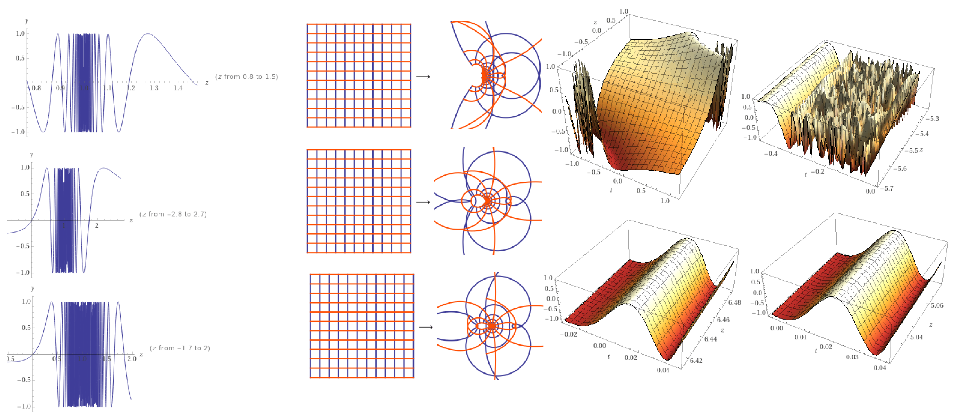
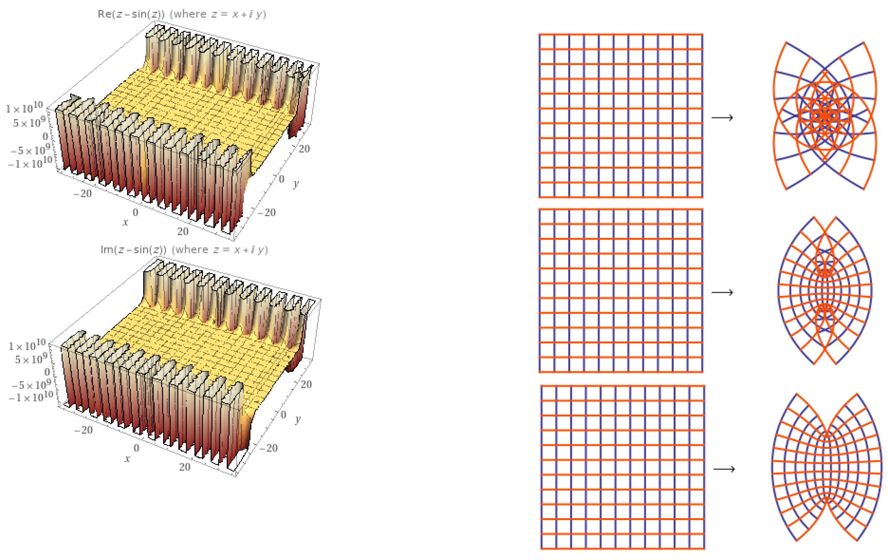
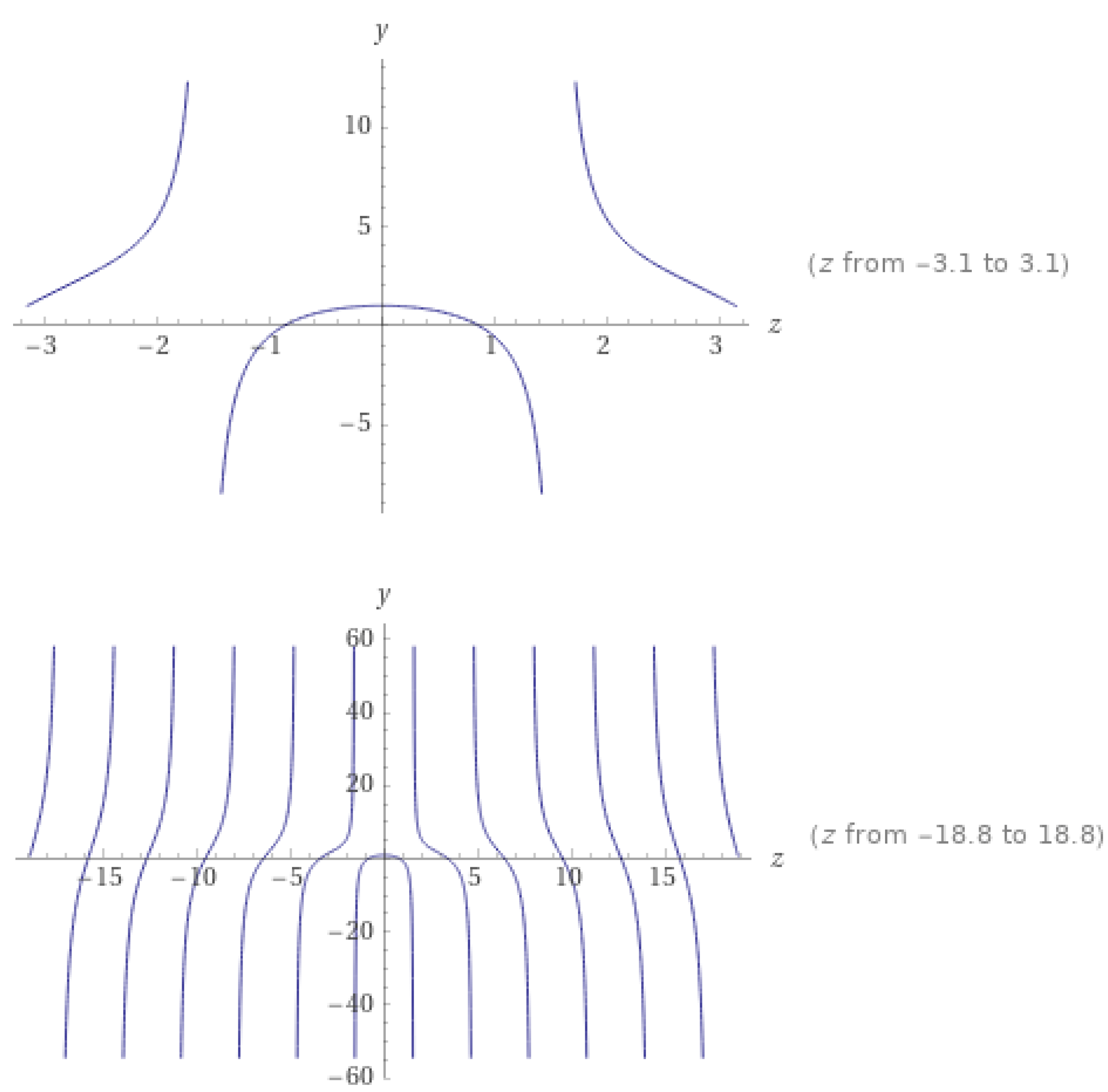
3.2. Dominated Solutions by a Chaotic Function

Next propositions indicate different conditions for the upper bound solutions of the wave Equations (6) and (7).

Proposition 4.

If ${}^{\mathfrak{R}}\left({\mathcal{S}}_{ð}^{\nu }\right)f(t,z)$ and ${}^{\mathfrak{C}}\left({\mathcal{S}}_{ð}^{\nu }\right)f(t,z)$ satisfy

$$z^2{{[}^{\mathfrak{R}}\left({\mathcal{S}}_{ð}^{\nu }\right)f(t,z)]}_{zz}+♭\left(z\right)z{{[}^{\mathfrak{R}}\left({\mathcal{S}}_{ð}^{\nu }\right)f(t,z)]}_z+{[}^{\mathfrak{R}}\left({\mathcal{S}}_{ð}^{\nu }\right)f(t,z)]\prec sin\left({\displaystyle \frac{z}{{(1-tz)}^{\varsigma }}}\right)$$

(15)

and

$$z^2{{[}^{\mathfrak{C}}\left({\mathcal{S}}_{ð}^{\nu }\right)f(t,z)]}_{zz}+♭\left(z\right)z{{[}^{\mathfrak{C}}\left({\mathcal{S}}_{ð}^{\nu }\right)f(t,z)]}_z+{[}^{\mathfrak{C}}\left({\mathcal{S}}_{ð}^{\nu }\right)f(t,z)]\prec sin\left({\displaystyle \frac{z}{{(1-tz)}^{\varsigma }}}\right)$$

(16)

respectively then for $t\to 1$ and $\Re (♭(z\left)\right)\ge 1,$ the inequalities

$${[}^{\mathfrak{R}}\left({\mathcal{S}}_{ð}^{\nu }\right)f(t,z)]\prec sin\left({\displaystyle \frac{z}{{(1-tz)}^{\varsigma }}}\right)$$

(17)

and

$${[}^{\mathfrak{C}}\left({\mathcal{S}}_{ð}^{\nu }\right)f(t,z)]\prec sin\left({\displaystyle \frac{z}{{(1-tz)}^{\varsigma }}}\right)$$

(18)

are occurred and $sin\left({\displaystyle \frac{z}{{(1-tz)}^{\varsigma }}}\right)$ is the best dominate whenever $\left|z\right|<0.86033$.

Proof. 

For $t\to 1,$ and in view of Proposition 1, the operators ${}^{\mathfrak{R}}\left({\mathcal{S}}_{ð}^{\nu }\right)f(t,z)$ and ${}^{\mathfrak{C}}\left({\mathcal{S}}_{ð}^{\nu }\right)f(t,z)$ are in the class $\mathsf{\Lambda }.$ Moreover,

$$sin{\left({\displaystyle \frac{z}{{(1-tz)}^{\varsigma }}}\right)}_{|z=0}=0,{[sin\left({\displaystyle \frac{z}{{(1-tz)}^{\varsigma }}}\right)]}_{z|z=0}=1.$$

A computation leads to (see Figure 3)

$$\Re \left(1+{\displaystyle \frac{z{[sin\left({\displaystyle \frac{z}{{(1-tz)}^{\varsigma }}}\right)]}_{zz}}{{[sin\left({\displaystyle \frac{z}{{(1-tz)}^{\varsigma }}}\right)]}_z}}\right)>0,\left|z\right|<0.86033;$$

thus $sin\left({\displaystyle \frac{z}{{(1-tz)}^{\varsigma }}}\right)$ is convex in the disk $\left|z\right|<0.86033.$

Then in view of [5]—Theorem 4.1e, the relations (15) and (16) imply the inequalities (17) and (18) respectively. □

Proposition 5.

If ${}^{\mathfrak{R}}\left({\mathcal{S}}_{ð}^{\nu }\right)f(t,z)$ and ${}^{\mathfrak{C}}\left({\mathcal{S}}_{ð}^{\nu }\right)f(t,z)$ satisfy

$$z{{[}^{\mathfrak{R}}\left({\mathcal{S}}_{ð}^{\nu }\right)f(t,z)]}_z\prec z{[sin\left({\displaystyle \frac{z}{{(1-tz)}^{\varsigma }}}\right)]}_z$$

(19)

and

$$z{{[}^{\mathfrak{C}}\left({\mathcal{S}}_{ð}^{\nu }\right)f(t,z)]}_z\prec z{[sin\left({\displaystyle \frac{z}{{(1-tz)}^{\varsigma }}}\right)]}_z$$

(20)

respectively then for $t\to 1$

$${[}^{\mathfrak{R}}\left({\mathcal{S}}_{ð}^{\nu }\right)f(t,z)]\prec sin\left({\displaystyle \frac{z}{{(1-tz)}^{\varsigma }}}\right)$$

(21)

and

$${[}^{\mathfrak{C}}\left({\mathcal{S}}_{ð}^{\nu }\right)f(t,z)]\prec sin\left({\displaystyle \frac{z}{{(1-tz)}^{\varsigma }}}\right).$$

(22)

And $sin\left({\displaystyle \frac{z}{{(1-tz)}^{\varsigma }}}\right)$ is the best dominate when $\left|z\right|<\pi /2$.

Proof. 

Since when $t\to 1,$ the operators ${}^{\mathfrak{R}}\left({\mathcal{S}}_{ð}^{\nu }\right)f(t,z)$ and ${}^{\mathfrak{C}}\left({\mathcal{S}}_{ð}^{\nu }\right)f(t,z)$ are in the class $\mathsf{\Lambda };$ and $z{[sin\left({\displaystyle \frac{z}{{(1-tz)}^{\varsigma }}}\right)]}_z$ is starlike in the disk $\left|z\right|<\pi /2$ [17], then in view of [5]—Corollary 3.4h.1, the relations (19) and (20) hit the inequalities (21) and (22) coordinately. □

4. Conclusions

From the above study, we introduced a new method for finding the analytic chaotic solution of a class of the symmetric wave equations defined by a symmetric fractional differential operator (SFDO) of a convex structure. The solution was suggested to be univalent (1-1) in the open unit disk. Moreover, under certain conditions, it was starlike. In addition, we formulated a fractional time wave equation by using the Riemann–Liouville derivative. We have utilized different techniques including majorization and subordination theory. The above approach can be used in various classes of physical equations like the Schrodinger equation. For future works, one can suggest different classes of analytic functions such as meromorphic functions, multivalent functions and harmonic functions.

References

1. Li, P.; Malomed, B.A.; Mihalache, D. Symmetry breaking of spatial Kerr solitons in fractional dimension. Chaos Solitons Fractals 2020, 132, 109602. [Google Scholar] [CrossRef] [Green Version]
2. Rusin, R.; Marangell, R.; Susanto, H. Symmetry breaking bifurcations in the NLS equation with an asymmetric delta potential. Nonlinear Dyn. 2020, 100, 3815–3824. [Google Scholar] [CrossRef]
3. Yagasaki, K.; Yamazoe, S. Numerical analyses for spectral stability of solitary waves near bifurcation points. Jpn. J. Ind. Appl. Math. 2021, 38, 125–140. [Google Scholar] [CrossRef]
4. Sa, L.; Ribeiro, P.; Prosen, T. Complex spacing ratios: A signature of dissipative quantum chaos. Phys. Rev. 2020, 10, 021019. [Google Scholar] [CrossRef]
5. Miller, S.S.; Mocanu, P.T. Differential Subordinations: Theory and Applications; CRC Press: Boca Raton, FL, USA, 2000. [Google Scholar]
6. MacGregor, T.H. Majorization by univalent functions. Duke Math. J. 1967, 43, 95–102. [Google Scholar] [CrossRef]
7. Fernandez, A. A complex analysis approach to Atangana-Baleanu fractional calculus. Math. Methods Appl. Sci. 2019, 44, 8070–8087. [Google Scholar] [CrossRef] [Green Version]
8. Shukla, A.K.; Prajapati, J.C. On a generalization of Mittag-Leffler function and its properties. J. Math. Anal. Appl. 2007, 336, 797–811. [Google Scholar] [CrossRef] [Green Version]
9. Haubold, H.J.; Mathai, A.M.; Saxena, R.K. Mittag-Leffler functions and their applications. J. Appl. Math. 2011, 2011, 298628. [Google Scholar] [CrossRef] [Green Version]
10. Godula, J.; Starkov, V.V. Sharpness of certain Campbell and Pommerenke estimates. Math. Notes 1998, 63, 586–592. [Google Scholar] [CrossRef]
11. Campbell, D.M. Majorization-subordination theorems for locally univalent functions, II. Can. J. Math. 1973, 25, 420–425. [Google Scholar] [CrossRef]
12. Ibrahim, R.W.; Baleanu, D. On quantum hybrid fractional conformable differential and integral operators in a complex domain. In Revista de la Real Academia de Ciencias Exactas, Fisicas y Naturales. Serie A. Matemáticas; Springer: Berlin, Germany, 2021; Volume 115, pp. 1–13. [Google Scholar]
13. Ibrahim, R.W.; Baleanu, D. On a combination of fractional differential and integral operators associated with a class of normalized functions. AIMS Math. 2021, 6, 4211–4226. [Google Scholar] [CrossRef]
14. Ibrahim, R.W.; Elobaid, R.M.; Obaiys, S.J. Generalized Briot-Bouquet differential equation based on new differential operator with complex connections. Axioms 2020, 9, 42. [Google Scholar] [CrossRef]
15. Ibrahim, R.W.; Elobaid, R.M.; Obaiys, S.J. On subclasses of analytic functions based on a quantum symmetric conformable differential operator with application. Adv. Differ. Equ. 2020, 2020, 325. [Google Scholar] [CrossRef]
16. Ibrahim, R.W.; Baleanu, D. Analytic Solution of the Langevin Differential Equations Dominated by a Multibrot. Fractal Set. Fractal Fract. 2021, 5, 50. [Google Scholar] [CrossRef]
17. Goodman, A.W. An invitation to the study of univalent and multivalent functions. Intr. Nat. J. Hath. Mh. Sci. 1979, 2, 163–186. [Google Scholar]
Figure 1. The plot of sin ( z / ( 1 t z ) ς ) , when t = 1 , ς = 1 , 2 , 3 . The last two columns are 2D plot for ς = 1 , 2 , 3 , 4 .
Axioms 10 00141 g001
Figure 2. Plot of the solution of Equation (11), when K = 1, 2, 3 in mesh mode respectively.
Axioms 10 00141 g002
Figure 3. Plot of 1 + z [ sin z ( 1 t z ) ς ] z z [ sin z ( 1 t z ) ς ] z , which shows the convexity of sin z ( 1 t z ) ς in the disk | z | < 0.86033 .
Axioms 10 00141 g003
Publisher’s Note: MDPI stays neutral with regard to jurisdictional claims in published maps and institutional affiliations.