1. Introduction
Maintenance comprises a set of procedures and methods for keeping a system in an operational state or returning the system to a functional state after failure [
1]. Depending on the activity and time for their implementation, maintenance can be corrective or preventive. Corrective maintenance implies a set of activities to be undertaken after a system stopped working, i.e., stopped performing its main function. In other words, the corrective maintenance activities are to be implemented only in cases of failure occurring as a result of an error (human, procedural or an error made by testing equipment), due to deterioration, environmental effect or damage caused by improper handling. In this category of maintenance, repairing or replacing a part, not before the exact moment of failure, is considered more efficient. The preventive maintenance implies periodical checking of the system’s conditions and parameters to prevent the occurrence of failure. This concept of preventive maintenance is based on the supervision and control of the system’s conditions while it is still in function and on the undertaking of those activities which delay the occurrence of failure and keep the system in its operational state. Since the occurrences of unplanned failures and damage to the system are almost unavoidable, even in cases when a system is regularly maintained, corrective maintenance should not be disregarded. All activities, whether in the form of preventive or corrective maintenance, require a certain period for their implementation. This time frame is usually called downtime and refers to a period when the observed component or system is not available. Because a large number of factors influence the duration of delay, these can be divided into waiting and active downtimes. The waiting downtimes are delays that occur due to waiting for spare parts, administrative procedures, deliveries, staff, etc. The active downtime refers to the time used for the repair or replacement of a component or system. As numerous factors can affect the time for repair, we can conclude that it is a random variable. Systems or components are divided into repairable and non-repairable. In non-repairable systems, the distribution of time to failure is most commonly observed. Many authors have dealt with these issues in their papers [
2,
3,
4]. On the other hand, there are repairable systems, i.e., systems that can be returned to their functional state with certain activities, after the occurrence of failure. The key performance measures of both repairable and non-repairable systems are availability and reliability. The availability is defined as a probability that a system will perform its function in a time [
5]. When it comes to military aircraft and weapon industry, availability can be defined as “a measure of the degree to which an item is in an operable state and can be committed at the start of a mission when the mission is called for at an unknown (random) point in time” [
6].
Maintenance contracts are most likely utilized when the system’s availability is vital. Their characteristic is that no specific maintenance activities such as servicing, repairs and required materials are paid for, but only the performances of the system result from the undertaking maintenance activities. This concept originates from the military industry, i.e., it is related to the maintenance of military aircraft and weapon systems. These types of contracts are called performance-based logistic (PBL) contracts. In other words, it is a strategy utilized in complex systems to lower maintenance expenses and increase their reliability and availability [
7]. Maintenance contracts have also found their use in civilian companies, under the name performance-based contracts (PBC) [
8]. In practice, when the airplane’s engine is serviced under the PBL contract, maintenance is not charged by the number of working hours used for engine repair or by the number of used spare parts, but by the time during which the airplane is available after repairs i.e., number of hours the engine is in the operational state [
9]. Kang et al. [
10] have observed systems whose maintenance was regulated with PBL contracts. They concluded that the mean time between failures (MTBF), mean time To repair (MTTR) and the number of spare parts have the greatest impact on availability. Evaluating the availability of a certain component or system is a common topic in the related literature. Inherited availability and methods for its evaluation in repairable systems have been researched in papers [
11,
12,
13]. Papers [
9,
14,
15,
16] provided major contributions concerning the issue of calculating the availability of repairable systems and operating under the maintenance contracts. Moreover, some control problems with interval analysis are presented in [
17,
18] and some statistical analyses that can be used for this purpose are presented in [
19,
20]. A similar issue was researched in paper [
21], in which it was concluded that the repair time and reliability have a significantly greater effect on the system’s availability than the number of spare parts in the inventory. Thus, according to reviewed literature, it can be concluded that the reliability and repair rate have the greatest impact on availability. In this paper, we observed a system modeled using an alternating renewal process and we analyzed the system repair rate in order to provide support in decision-making process when it comes to system maintenance planning. The main contribution of our paper is the new method that relies on the observation of the annual repair rate. This method was based on the determination of the maximal repair rate of units that compose a corresponding entity, including its magnitude and performance measures that unambiguously define the total repair rate of an observed entity and which have not been discussed in renewal theory literature to date. We calculated two new parameters that are interesting for the observation, maximal and minimal repair rate of each unit that constitute the corresponding entity by observing them as stochastic variables. In this way, we obtained analytical expressions that can be used to predict the total repair time of the corresponding entity. These generalized PDF expressions are our main contribution.
2. Mathematical Method for System Repair Rate Analysis
The stochastic modeling of a component or system repair time is not new and has already been justified in the paper [
22]. There, the author emphasizes the importance of the stochastic modeling of the system maintenance by observing a one-unit reparable system with a non-negligible repair time. The homogeneous, nonhomogeneous and compound Poisson process for system maintenance modeling was investigated. In this paper, we used a model presented in [
23], where the authors studied similar systems such as that in [
22] with the assumption that the MTBF is Rayleigh distributed. Based on these assumptions, they investigated the repair rate in dependence of the desired level of availability. Only repairable components and systems were taken into consideration, i.e., the systems that alternate between successive up and down intervals. Thus, the alternating renewal process [
24] was used to model such a system. This process can be observed as a series of independent and non-negative random variables such as the time to failure and time to repair. It was assumed that each time the failure occurs, the component will be restored and start to behave the same as the new one. Notably, we only observed perfect repair, although in the literature and in practice, there are two types of repair: perfect and imperfect. While perfect repair means that the unit can be reused in the state “as good as new”, imperfect repair is defined as an action after which the unit is not “as good as new” but it is in usable/operational condition.
The purpose of maintenance contracts is to reduce the costs and increase system availability that can be further calculated as expected operative time
and a renewal cycle (
i.e., sum of the expected operative time and time to repair) [
25]:
The expected operative time is a random variable which, if probability density function exists, can be calculated as
In [
4], the authors assumed that this variable is Rayleigh distributed with the following probability density function (PDF):
Assuming that the expected time to failure of the component is a Rayleigh-distributed random variable, the authors provided the expression for the PDF of the repair rate in dependence of unit’s availability as
where
A is availability,
is the repair rate, and
. Based on Equation (
4), the cumulative probability density function CDF can be expressed as
Based on these calculations for a single component or subsystem, in this paper, we proposed a new model for calculating the maximal and minimal repair rate of the system comprised of two or more components. The PDF function of the first component is:
where
is the set level of availability of the first unit and, i.e., the mathematical expectation of the Rayleigh-distributed parameter for that component. The cumulative density function (CDF) is then:
Using the same equation, we can determine the PDF of the second unit
with availability
and
as
and the CDF:
For a system composed of two parts, we can calculate the maximal repair rate as
. In that case, the PDF is:
while the CDF is:
Furthermore, when a system is comprised of n parts, then the repair rate can be calculated as
. The general form of the repair rate’s PDF is then:
and the general form of the CDF is:
Similarly, we can calculate the minimal repair rate as
, so the PDF is:
while the CDF is:
General forms of the PDF and CDF equations when the system is comprised of n parts and repair rate is
are:
and the general form of the CDF for this system is:
3. Numerical Results and Discussions
To verify the model presented in the previous section, we used the data calculated in [
10,
21]. In these papers, the authors observed the unmanned aerial vehicle (UAV), i.e., its three major components: engine, propeller and avionics. The available data of the major interest for our paper are as follows:
- -
Each UAV is supposed to have 120 flight hour per month, which further means 1440 flight hours per year;
- -
MTBF for UAV’s engine is 750 flight hours, while for avionics this is 1000 h and 500 h for propeller per year.
- -
Thus, based on that in [
21], the failure rate was calculated as 1.92 (failures per year) for the engine, 2.88 for the propeller and 1.44 for avionics.
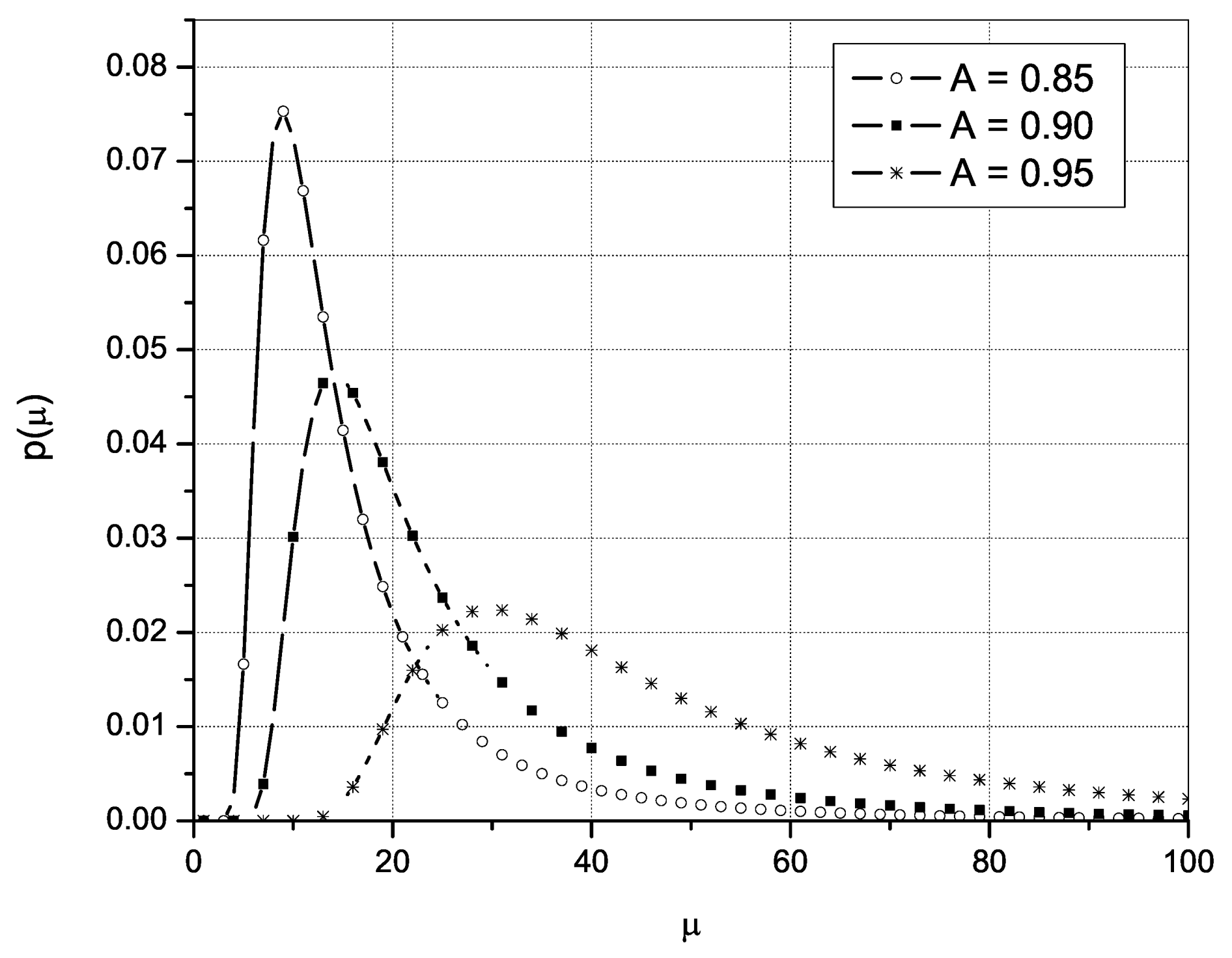
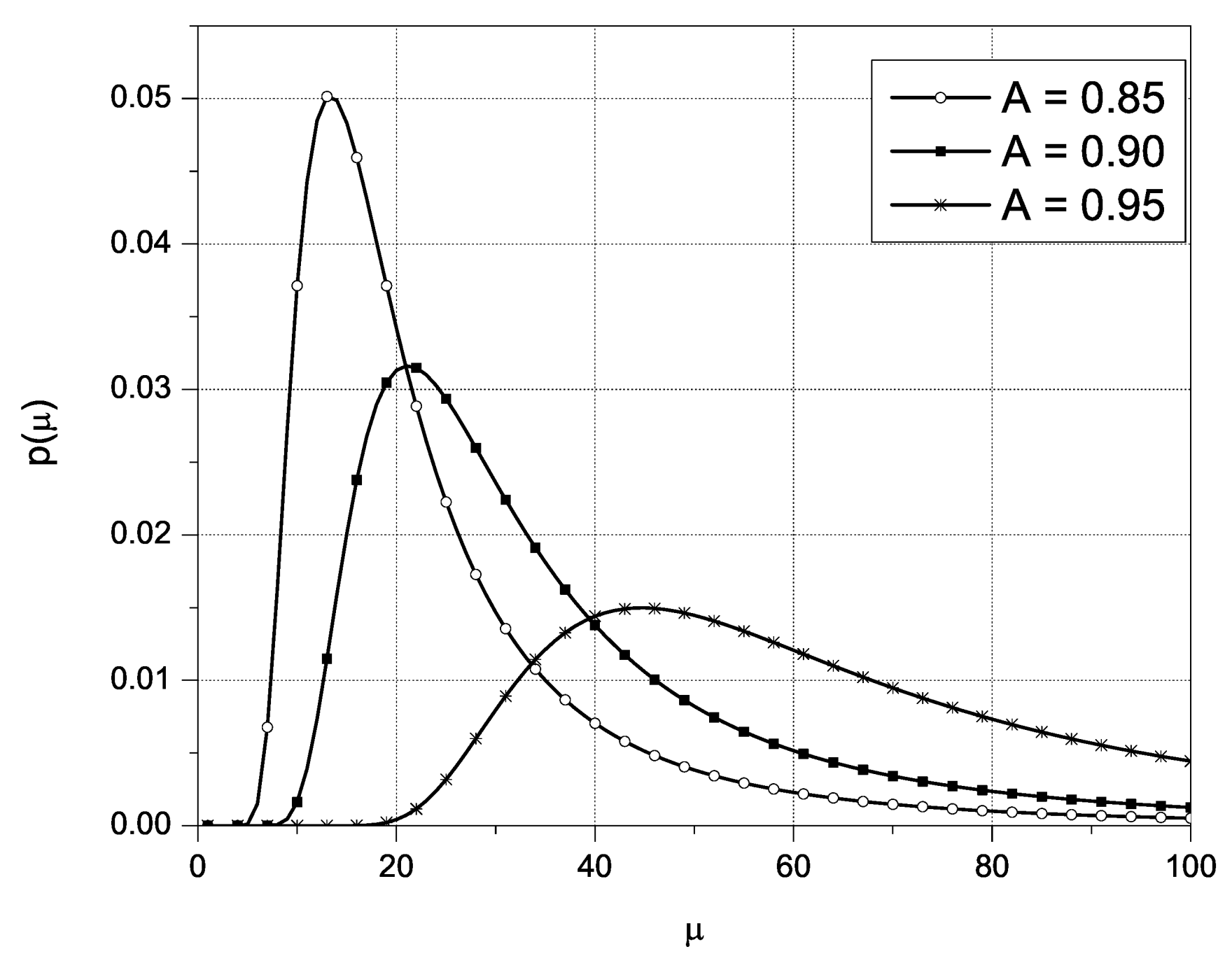
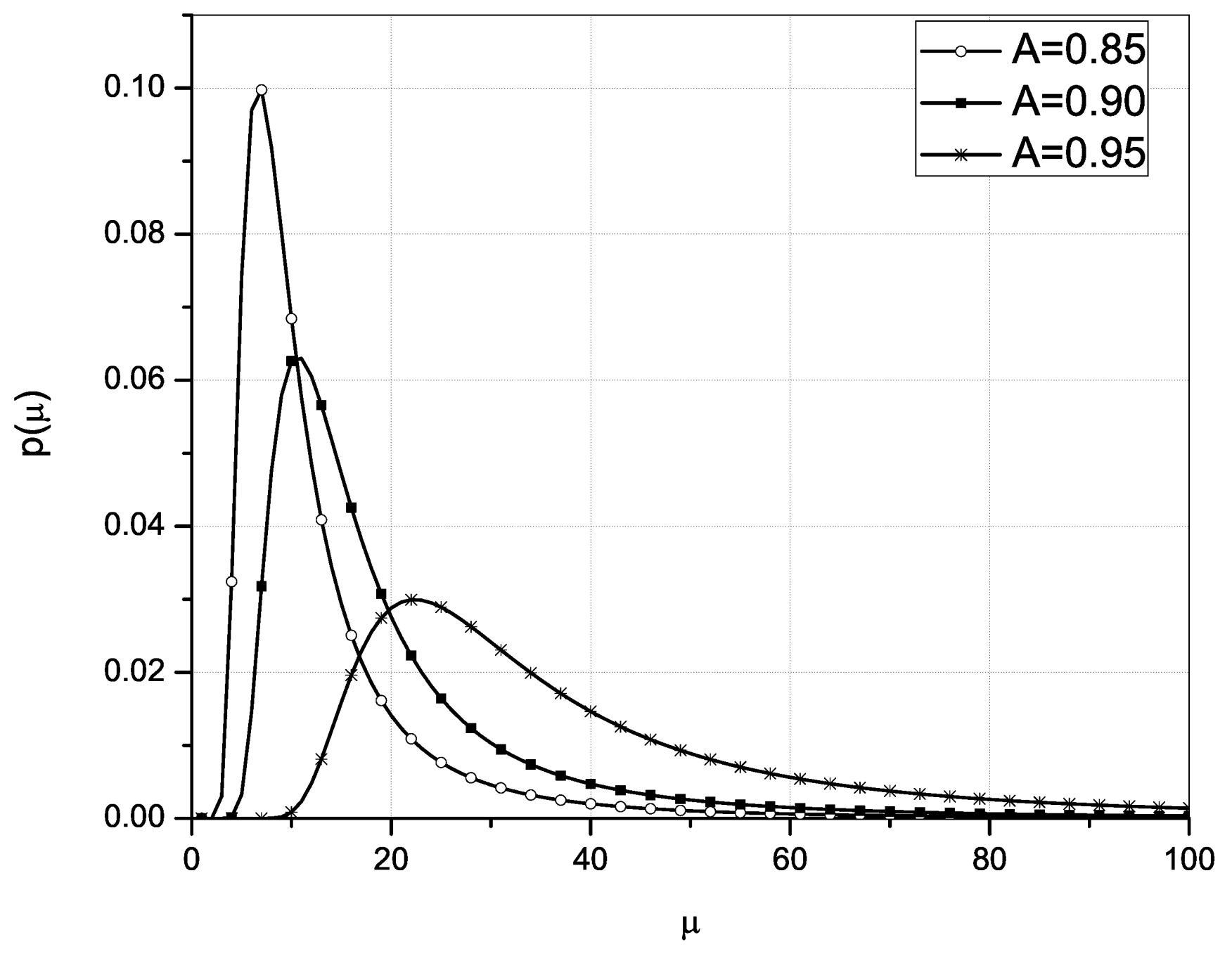
As can be seen, all three figures present the PDF of the UAV’s engine, propeller and avionics, respectively, for different values of availability (any other value could also be selected).
As the availability A increases, the maximum PDF values moves to the right, which further means that maximum PDF values are obtained for higher annual repair rate values, i.e., as A grows a higher value of
is needed to achieve maximum PDF. For example, as it can be seen on
Figure 1 that present maximum annual repair rate in dependence of availability for UAV’s engine, to achieve the availability of 85% the number of repairs per year should be around 10, for availability of 90% the repair rate should be around 15 and for 95% it should be around 30. The same interpretation could be given for
Figure 2 and
Figure 3 that presents the dependence of the annual repair rate of availability for UAV’s propeller and avionics.
Similarly, we can calculate the annual expected time for the maximum and minimum repair rate of the UAV system. We have to take into consideration all three critical components of the UAV system: engine, propeller and avionics. Here, we set the availability at
. Since in this case we are observing a system comprised of three critical UAV components, the PDF maximal repair rate can be calculated as:
According to the Equation (
12), the PDF of the repair rate is:
while the CDF is:
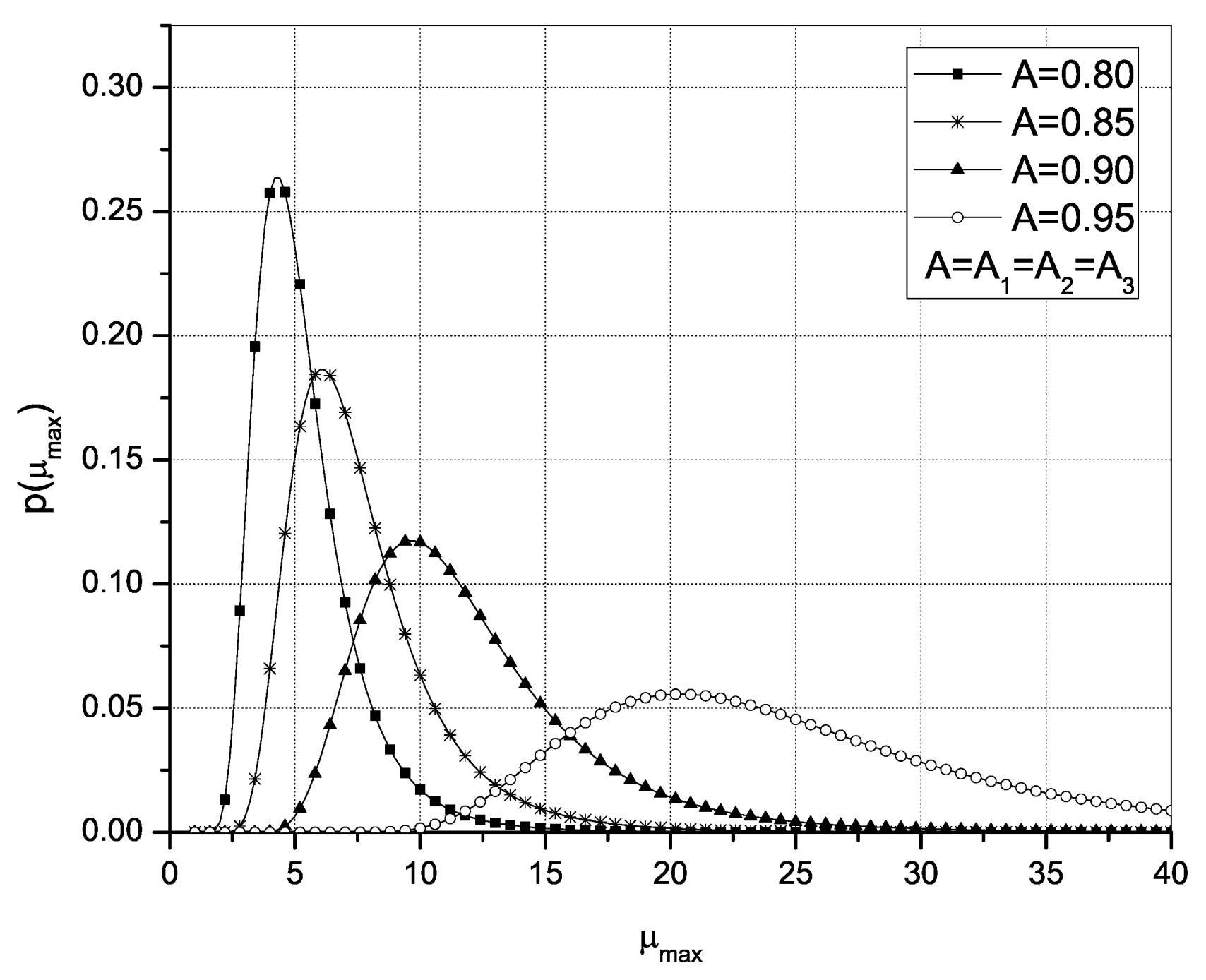
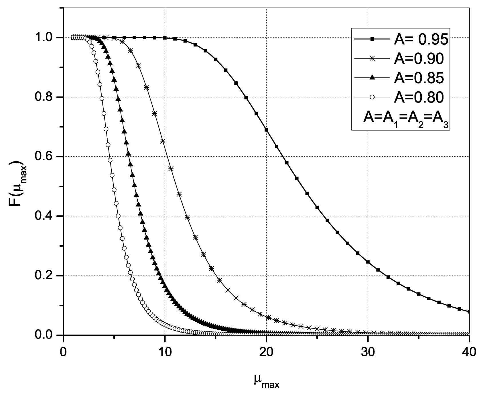
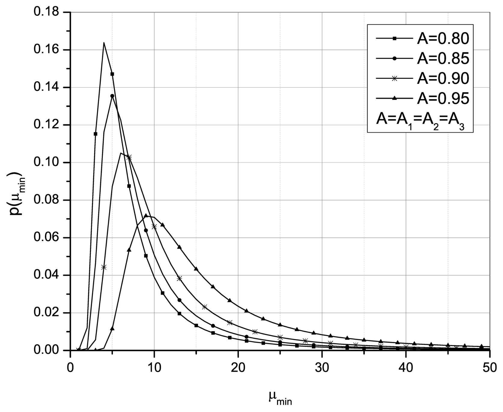
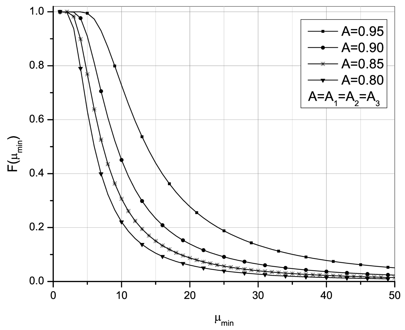
Figure 4 and
Figure 5 represent the PDF and CDF, respectively, of the UAV’s repair rate depending on time; the repair rate was calculated as the maximum of its components’ repair rate and based on the presented equations. The desired level of availability is set to 80%, 85%, 90% and 95%. Actually, in
Figure 4, we observed the magnitude of the maximum repair rate of the system comprised of the engine, propeller and avionics. It can be seen that the maximum PDF of this parameter shifts to the right again as the value of availability increases, which means that with the higher values of
A, the maximum value of the repair rate of the whole system is more likely to take on a higher value.
Figure 5 shows that for smaller values of
A, the range of values that the maximum repair rate could take is smaller, but when the availability increases, the range that maximum repair rate values can take also increases.
Similarly, we can determine the minimal repair rate of the observed UAV, comprised of three critical components as
, so the PDF is:
while the CDF is:
Figure 6 and
Figure 7 represent the PDF and CDF, respectively, of the UAV’s repair rate depending on time and the repair rate is calculated as the minimum of its components’ repair rate. The desired level of availability is set to 80%, 85%, 90% and 95% as in the previous example. From
Figure 6 and
Figure 7, we can also see that as the
A parameter increases, the maximum PDF values migrate to the right as in previous case. However when compared to
Figure 4 and
Figure 5 we can see that for the same values of parameter
A, maximum PDF values are obtained for lower annual repair rate values and this repair rate value represents lower system performance bound for observed entity. The presented figures show the probability that the repairs conducted in a certain time frame will provide the desired level of system availability.
4. Conclusions
The analysis presented in this paper can be applied to other repairable systems, not only to ones where the component time to failure is modeled with Rayleigh distribution. After determining the characteristics of the repair rate of an individual unit, the statistical analysis of the repair rate of a system consisting of several components is presented, which was the main contribution of this paper. Actually, a novel method for the determination of the maximal and minimal repair rate of the entity comprised of the observed units is presented. The obtained generalized PDF expressions can be used to predict total repair time. The presented method provides two new measures that comprehensively define the total repair time and have not been studied in this way before. In the numerical section, the proposed model was applied to a UVA system consisting of three key components: the motor, propeller, and avionics. PDFs of repair rate for each component, as well as the PDF and CDF maximum and minimum repair rates for the entire UAV system. The obtained information is graphically presented and it can be concluded that as that maximum PDF values are obtained for higher annual repair rate values as the availability increases, i.e., as A grows, a higher value of repair rate is needed to achieve a maximum PDF. The similar behavior is noticed when we observed the minimal annual repair rate but in this case the maximum PDF values are obtained for lower annual repair rate values and this repair rate value represent a lower system performance bound for an observed entity. Based on that, we can predict the time interval by which the maintenance action will have to be successfully completed in order to achieve the desired level of availability. Although we set availability to certain levels, numerical analysis can be repeated with different availability values.


