Approximations of an Equilibrium Problem without Prior Knowledge of Lipschitz Constants in Hilbert Spaces with Applications

Abstract

The objective of this paper is to introduce an iterative method with the addition of an inertial term to solve equilibrium problems in a real Hilbert space. The proposed iterative scheme is based on the Mann-type iterative scheme and the extragradient method. By imposing certain mild conditions on a bifunction, the corresponding theorem of strong convergence in real Hilbert space is well-established. The proposed method has the advantage of requiring no knowledge of Lipschitz-type constants. The applications of our results to solve particular classes of equilibrium problems is presented. Numerical results are established to validate the proposed method’s efficiency and to compare it to other methods in the literature.

1. Introduction

Suppose that $\mathcal{C}$ is a nonempty closed and convex subset of a real Hilbert space $\mathcal{H}.$ The inner product and induced norm are denoted by $\langle ·,·\rangle$ and $\parallel ·\parallel$, respectively. Let $f:\mathcal{H}\times \mathcal{H}\to \mathcal{R}$ be a bifunction and $f(y,y)=0,$ for all $y\in \mathcal{C}.$ The equilibrium problem (EP) [1,2] for a bifunction f on $\mathcal{C}$ is defined in the following way:

$$\mathrm{Find}{u}^{*}\in \mathcal{C}\mathrm{such}\mathrm{that}f(u^{*},y)\ge 0,\forall y\in \mathcal{C}.$$

(EP)

The equilibrium problem is a general mathematical problem in the sense that it unifies various mathematical problems, i.e., fixed-point problems, vector and scalar minimization problems, problems of variational inequality, complementarity problems, Nash equilibrium problems in noncooperative games, saddle point problems, and inverse optimization problems [2,3,4]. The equilibrium problem is also known as the well-known Ky Fan inequality due to the result [1]. Many authors established and generalized several results on the existence and nature of the solution of the equilibrium problems (see for more detail [1,4,5]). Due to the importance of this problem (EP) in both pure and applied sciences, many researchers studied it in recent years [6,7,8,9,10,11,12,13,14,15,16,17] and other in [18,19,20,21,22].

Tran et al. in [23] introduced iterative sequence $\left\{u_n\right\}$ in the following way:

$$\left\{\begin{array}{c}{u}_0\in \mathcal{C},\hfill \\ y_n=\underset{z\in \mathcal{C}}{argmin}\{\chi f(u_n,z)+\frac{1}{2}\parallel u_n-z{\parallel }^2\},\hfill \\ u_{n+1}=\underset{z\in \mathcal{C}}{argmin}\{\chi f(y_n,z)+\frac{1}{2}\parallel u_n-z{\parallel }^2\},\hfill \end{array}\right.$$

(1)

where $0<\chi <min\left\{\frac{1}{2c_1},\frac{1}{2c_2}\right\}.$ This method is also known as the extragradient method in [23] due to the previous contribution of Korpelevich [24] to solve the saddle-point problems. The iterative sequence generated by the above-mentioned method is weakly convergent to the solution with prior knowledge of Lipschitz-type constants. These Lipschitz-like constants are often not known or are difficult to compute. Recently, Hieu et al. [25] introduced an extension of the method (1) for solving the equilibrium problem. Let us consider that ${\left[p\right]}_{+}:=max\{p,0\}$ and choose $u_0\in \mathcal{C},$$\mu \in (0,1)$ with ${\chi }_0>0$ such that

$$\left\{\begin{array}{c}{y}_n=\underset{z\in \mathcal{C}}{argmin}\{{\chi }_{n}f(u_n,z)+\frac{1}{2}\parallel u_n-z{\parallel }^2\},\hfill \\ u_{n+1}=\underset{z\in \mathcal{C}}{argmin}\{{\chi }_{n}f(y_n,z)+\frac{1}{2}\parallel u_n-z{\parallel }^2\},\hfill \end{array}\right.$$

(2)

where $\left\{{\chi }_n\right\}$ is updated in the following manner:

$${\chi }_{n+1}=min\left\{{\chi }_n,\frac{\mu (\parallel u_n-y_n{\parallel }^2+\parallel u_{n+1}-y_n{\parallel }^2)}{2{[f(u_n,u_{n+1})-f(u_n,y_n)-f(y_n,u_{n+1})]}_{+}}\right\}.$$

Inertial-like methods are well-known two-step iterative methods in which the next iteration is derived from the previous two iterations (see [26,27] for more details). To speed up the iterative sequence convergence rate, an inertial extrapolation term is used. Numerical examples show that inertial effects improve numerical performance in terms of execution time and the expected number of iterations. Recently, many existing methods were established for the case of equilibrium problems (see [28,29,30,31] for more details).

In this paper, inspired by the methods in [23,25,26,32], we introduce a general inertial Mann-type subgradient extragradient method to evaluate the approximate solution of the equilibrium problems involving pseudomonotone bifunction. A strong convergence result corresponding to the proposed algorithm is well-established by assuming certain mild conditions. Some of the applications for our main results are considered to solve the fixed-point problems. Lastly, computational results show that the new method is more successful than existing ones [23,33,34].

2. Preliminaries

A metric projection $P_{\mathcal{C}}\left(u\right)$ of $u\in \mathcal{H}$ onto a closed and convex subset $\mathcal{C}$ of $\mathcal{H}$ is defined by

$$P_{\mathcal{C}}\left(u\right)=\underset{y\in \mathcal{C}}{argmin}\{\parallel y-u\parallel \}.$$

In this study, the equilibrium problem under the following conditions:

(c1).

A bifunction $f:\mathcal{H}\times \mathcal{H}\to \mathcal{R}$ is said to be pseudomonotone [3,35] on $\mathcal{C}$ if

$$f(y_1,y_2)\ge 0⟹f(y_2,y_1)\le 0,\forall y_1,y_2\in \mathcal{C}.$$

(c2).

A bifunction $f:\mathcal{H}\times \mathcal{H}\to \mathcal{R}$ is said to be Lipschitz-type continuous [36] on $\mathcal{C}$ if there exist constants $c_1,c_2>0$ such that

$$f(y_1,y_3)\le f(y_1,y_2)+f(y_2,y_3)+c_1\parallel y_1-y_2{\parallel }^2+c_2{\parallel y_2-y_3\parallel }^2,\forall y_1,y_2,y_3\in \mathcal{C}.$$

(c3).

$\underset{n\to \infty }{lim\; sup}f(y_n,y)\le f(q^{*},y)$ for all $y\in \mathcal{C}$ and $\left\{y_n\right\}\subset \mathcal{C}$ satisfy $y_n\rightharpoonup q^{*}.$

(c4).

$f(u,·)$ is convex and subdifferentiable on $\mathcal{H}$ for each $u\in \mathcal{H}.$

A cone on $\mathcal{C}$ at $u\in \mathcal{C}$ is defined by

$$N_{\mathcal{C}}\left(u\right)=\{t\in \mathcal{H}:\langle t,y-u\rangle \le 0,\forall y\in \mathcal{C}\}.$$

Let a convex function $\daleth :\mathcal{C}\to \mathcal{R}$ and subdifferential of ℸ at $u\in \mathcal{C}$ is defined by

$$\partial \daleth \left(u\right)=\{t\in \mathcal{H}:\daleth (y)-\daleth (u)\ge \langle t,y-u\rangle ,\forall y\in \mathcal{C}\}.$$

Lemma 1.

 [37] Let $\daleth :\mathcal{C}\to \mathcal{R}$ be a subdifferentiable, lower semicontinuous, and convex function on $\mathcal{C}$. Then, $u\in \mathcal{C}$ is said to be a minimizer of ℸ if and only if $0\in \partial \daleth \left(u\right)+N_{\mathcal{C}}\left(u\right)$, where $\partial \daleth \left(u\right)$ stands for the subdifferential of ℸ at $u\in \mathcal{C}$ and $N_{\mathcal{C}}\left(u\right)$ is a normal cone of $\mathcal{C}$ on $u.$

Lemma 2.

 [38] Assume that $P_{\mathcal{C}}:\mathcal{H}\to \mathcal{C}$ be a metric projection such that

(i)

$\parallel y_1-P_{\mathcal{C}}\left(y_2\right){\parallel }^2+\parallel P_{\mathcal{C}}\left(y_2\right)-y_2{\parallel }^2\le {\parallel y_2-y_1\parallel }^2,y_1\in \mathcal{C},y_2\in \mathcal{H}.$  

(ii)

$y_3=P_{\mathcal{C}}\left(y_1\right)$ if and only if $\langle y_1-y_3,y_2-y_3\rangle \le 0,\forall y_2\in \mathcal{C}.$  

(iii)

$\parallel y_1-P_{\mathcal{C}}\left(y_1\right)\parallel \le \parallel y_1-y_2\parallel ,y_2\in \mathcal{C},y_1\in \mathcal{H}.$

Lemma 3.

 [39] Assume that $\left\{{\daleth }_n\right\}\subset (0,+\infty )$ is a sequence satisfying, i.e., ${\daleth }_{n+1}\le (1-{\mho }_n){\daleth }_n+{\mho }_n{ð}_n,\mathrm{for}\mathrm{all}n\in \mathbb{N}.$ Moreover, let $\left\{{\mho }_n\right\}\subset (0,1)$ and $\left\{{ð}_n\right\}\subset \mathcal{R}$ be two sequences, such that ${lim}_{n\to \infty }{\mho }_n=0,{\sum }_{n=1}^{\infty }{\mho }_n=+\infty and{lim\; sup}_{n\to \infty }{ð}_n\le 0.$ Then, ${lim}_{n\to \infty }{\daleth }_n=0.$

Lemma 4.

 [40] Assume that $\left\{{\daleth }_n\right\}$ be a sequence of real numbers such that there exists a subsequence $\left\{n_i\right\}$ of $\left\{n\right\}$ such that ${\daleth }_{n_i}<{\daleth }_{n_{i+1}}$ for all $i\in \mathbb{N}.$ Then, there is a nondecreasing sequence $m_k\subset \mathbb{N}$ such that $m_k\to \infty$ as $k\to \infty ,$ and the following conditions are fullfiled by all (sufficiently large) numbers $k\in \mathbb{N}$:

$${\daleth }_{m_k}\le {\daleth }_{m_{k+1}}\mathrm{and}{\daleth }_k\le {\daleth }_{m_{k+1}}.$$

In fact, $m_k=max\{j\le k:{\daleth }_j\le {\daleth }_{j+1}\}.$

Lemma 5.

[41] For all $y_1,y_2\in \mathcal{H}$ and $ð\in \mathcal{R},$ the following inequalities hold.

(i)

$\parallel ðy_1+(1-ð)y_2{\parallel }^2=ð\parallel y_1{\parallel }^2+(1-ð)\parallel y_2{\parallel }^2-ð(1-ð){\parallel y_1-y_2\parallel }^2.$  

(ii)

$\parallel y_1+y_2{\parallel }^2\le {\parallel y_1\parallel }^2+2\langle y_2,y_1+y_2\rangle$.

3. Main Results

We propose an iterative method for solving equilibrium problems involving a pseudomonotone that is based on Tran et al. in [23], and the Mann-type method [32] and the inertial scheme [26]. For clarity in the presentation, we use notation ${\left[t\right]}_{+}=max\{0,t\}$ and follow conventions $\frac{0}{0}=+\infty$ and $\frac{a}{0}=+\infty$$(a\ne 0).$

Lemma 6.

A sequence $\left\{{\chi }_n\right\}$ generated by (5) is monotonically decreasing, converges to $\chi >0$, and has a lower bound $min\left\{\frac{\mu }{2max\{c_1,c_2\}},{\chi }_0\right\}.$

Proof. 

Assume that $f(t_n,z_n)-f(t_n,y_n)-f(y_n,z_n)>0$ such that

$$\begin{array}{cc}\hfill \frac{\mu (\parallel t_n-y_n{\parallel }^2+\parallel z_n-y_n{\parallel }^2)}{2[f(t_n,z_n)-f(t_n,y_n)-f(y_n,z_n)]}& \ge \frac{\mu (\parallel t_n-y_n{\parallel }^2+\parallel z_n-y_n{\parallel }^2)}{2[c_1\parallel t_n-y_n{\parallel }^2+c_2\parallel z_n-y_n{\parallel }^2]}\hfill \\ \hfill & \ge \frac{\mu }{2max\{c_1,c_2\}}.\hfill \end{array}$$

(3)

This implies that $\left\{{\chi }_n\right\}$ has a lower bound $min\left\{\frac{\mu }{2max\{c_1,c_2\}},{\chi }_0\right\}.$ Moreover, there exists a fixed real number $\chi >0$, such that ${lim}_{n\to \infty }{\chi }_n=\chi .$ ☐

Lemma 7.

Suppose that Conditions (c1)–(c4) are satisfied. Then, sequence $\left\{u_n\right\}$ generated by the Algorithm 1 is a bounded sequence.

Algorithm 1 (Explicit Accelerated Strong Convergence Iterative Scheme)

Step 0: Choose $u_{-1},u_0\in \mathcal{C},$$\varphi >0$, ${\chi }_0>0$, $\left\{{\rho }_n\right\}\subset (a,b)\subset (0,1-{\varrho }_n)$ and $\left\{{\varrho }_n\right\}\subset (0,1)$ satisfies the following conditions: $$\underset{n\to \infty }{lim}{\varrho }_n=0and\sum _{n=1}^{+\infty }{\varrho }_n=+\infty .$$ Step 1: Compute $t_n=u_n+{\varphi }_n(u_n-u_{n-1})$ and choose ${\varphi }_n$ such that $$0\le {\varphi }_n\le \widehat{{\varphi }_n}\mathrm{and}\widehat{{\varphi }_n}=\left\{\begin{array}{cc}min\left\{\frac{\varphi }{2},\frac{{\varsigma }_n}{\parallel u_n-u_{n-1}\parallel }\right\}\hfill & \mathrm{if}{u}_n\ne u_{n-1},\frac{\varphi }{2}\hfill \\ \frac{\varphi }{2}\hfill & \mathrm{otherwise},\hfill \end{array}\right.$$ (4) where ${\varsigma }_n=\circ \left({\varrho }_n\right)$, i.e., ${lim}_{n\to \infty }\frac{{\varsigma }_n}{{\varrho }_n}=0.$ Step 2: Compute $$y_n=\underset{y\in \mathcal{C}}{argmin}\{{\chi }_{n}f(t_n,y)+\frac{1}{2}\parallel t_n-y{\parallel }^2\}.$$ If $t_n=y_n$, then STOP the sequence. Else, go to Step 3. Step 3: Construct a half-space ${\mathcal{H}}_n=\{z\in \mathcal{H}:\langle t_n-{\chi }_n{\omega }_n-y_n,z-y_n\rangle \le 0\}$ where ${\omega }_n\in {\partial }_{2}f(t_n,y_n)$ and compute $$z_n=\underset{y\in {\mathcal{H}}_n}{argmin}\{{\chi }_{n}f(y_n,y)+\frac{1}{2}\parallel t_n-y{\parallel }^2\}.$$ Step 4: Compute $u_{n+1}=(1-{\rho }_n-{\varrho }_n)u_n+{\rho }_n{z}_n.$ Step 5: Compute $${\chi }_{n+1}=min\left\{{\chi }_n,\frac{\mu \parallel t_n-y_n{\parallel }^2+\mu {\parallel z_n-y_n\parallel }^2}{2{[f(t_n,z_n)-f(t_n,y_n)-f(y_n,z_n)]}_{+}}\right\}.$$ (5) Set $n:=n+1$ and go back to Step 1.

Proof. 

From the value of $z_n,$ we have

$$0\in {\partial }_2\left\{{\chi }_{n}f(y_n,y)+\frac{1}{2}{\parallel t_n-y\parallel }^2\right\}\left(z_n\right)+N_{{\mathcal{H}}_n}\left(z_n\right).$$

For $\omega \in \partial f(y_n,z_n)$ there exists $\overline{\omega }\in N_{{\mathcal{H}}_n}\left(z_n\right)$ such that

$${\chi }_n\omega +z_n-t_n+\overline{\omega }=0.$$

This implies that

$$\langle t_n-z_n,y-z_n\rangle ={\chi }_n\langle \omega ,y-z_n\rangle +\langle \overline{\omega },y-z_n\rangle ,\forall y\in {\mathcal{H}}_n.$$

Due to $\overline{\omega }\in N_{{\mathcal{H}}_n}\left(z_n\right)$, it implies that $\langle \overline{\omega },y-z_n\rangle \le 0$ for each $y\in {\mathcal{H}}_n.$ Thus, we have

$$\langle t_n-z_n,y-z_n\rangle \le {\chi }_n\langle \omega ,y-z_n\rangle ,\forall y\in {\mathcal{H}}_n.$$

(6)

Moreover, $\omega \in \partial f(y_n,z_n)$ and owing to the subdifferential, we have

$$f(y_n,y)-f(y_n,z_n)\ge \langle \omega ,y-z_n\rangle ,\forall y\in \mathcal{H}.$$

(7)

From Expressions (6) and (7), we obtain

$${\chi }_{n}f(y_n,y)-{\chi }_{n}f(y_n,z_n)\ge \langle t_n-z_n,y-z_n\rangle ,\forall y\in {\mathcal{H}}_n.$$

(8)

Due to the definition of ${\mathcal{H}}_n$, we have

$${\chi }_n\langle {\omega }_n,z_n-y_n\rangle \ge \langle t_n-y_n,z_n-y_n\rangle .$$

(9)

Now, using ${\omega }_n\in \partial f(t_n,y_n)$, we obtain

$$f(t_n,y)-f(t_n,y_n)\ge \langle {\omega }_n,y-y_n\rangle ,\forall y\in \mathcal{H}.$$

By letting $y=z_n$, we obtain

$$f(t_n,z_n)-f(t_n,y_n)\ge \langle {\omega }_n,z_n-y_n\rangle ,\forall y\in \mathcal{H}.$$

(10)

Combining Expressions (9) and (10), we obtain

$${\chi }_n\left\{f(t_n,z_n)-f(t_n,y_n)\right\}\ge \langle t_n-y_n,z_n-y_n\rangle .$$

(11)

By substituting $y=u^{*}$ in Expression (8), we obtain

$${\chi }_{n}f(y_n,u^{*})-{\chi }_{n}f(y_n,z_n)\ge \langle t_n-z_n,u^{*}-z_n\rangle .$$

(12)

Since $u^{*}\in Ep(f,\mathcal{C})$, we have $f(u^{*},y_n)\ge 0.$ From the pseudomonotonicity of bifunction f, we achieve $f(y_n,u^{*})\le 0.$ It follows from Expression (12) that

$$\langle t_n-z_n,z_n-u^{*}\rangle \ge {\chi }_{n}f(y_n,z_n).$$

(13)

From the description of ${\chi }_{n+1},$ we obtain

$$f(t_n,z_n)-f(t_n,y_n)-f(y_n,z_n)\le \frac{\mu \parallel t_n-y_n{\parallel }^2+\mu {\parallel z_n-y_n\parallel }^2}{2{\chi }_{n+1}}$$

(14)

From (13) and (14), we obtain

$$\begin{array}{cc}\hfill \langle t_n-z_n,z_n-u^{*}\rangle & \ge {\chi }_n\{f(t_n,z_n)-f(t_n,y_n)\}\hfill \\ \hfill & -\frac{\mu {\chi }_n}{2{\chi }_{n+1}}\parallel t_n-y_n{\parallel }^2-\frac{\mu {\chi }_n}{2{\chi }_{n+1}}{\parallel z_n-y_n\parallel }^2.\hfill \end{array}$$

(15)

Combining Expressions (11) and (15), we have

$$\begin{array}{cc}\hfill \langle t_n-z_n,z_n-u^{*}\rangle & \ge \langle t_n-y_n,z_n-y_n\rangle \hfill \\ \hfill & -\frac{\mu {\chi }_n}{2{\chi }_{n+1}}\parallel t_n-y_n{\parallel }^2-\frac{\mu {\chi }_n}{2{\chi }_{n+1}}{\parallel z_n-y_n\parallel }^2.\hfill \end{array}$$

(16)

We have the given formula in place:

$$-2\langle t_n-z_n,z_n-u^{*}\rangle =-\parallel t_n-u^{*}{\parallel }^2+\parallel z_n-t_n{\parallel }^2+{\parallel z_n-u^{*}\parallel }^2.$$

(17)

$$2\langle y_n-t_n,y_n-z_n\rangle =\parallel t_n-y_n{\parallel }^2+\parallel z_n-y_n{\parallel }^2-{\parallel t_n-z_n\parallel }^2.$$

(18)

Combining (16)–(18), we obtain

$$\parallel z_n-u^{*}{\parallel }^2\le \parallel t_n-u^{*}{\parallel }^2-\left(1-\frac{\mu {\chi }_n}{{\chi }_{n+1}}\right)\parallel t_n-y_n{\parallel }^2-\left(1-\frac{\mu {\chi }_n}{{\chi }_{n+1}}\right){\parallel z_n-y_n\parallel }^2.$$

(19)

Since ${\chi }_n\to \chi ,$ then there is number $\Im \in (0,1-\mu )$ that

$$\underset{n\to \infty }{lim}\left(1-\frac{\mu {\chi }_n}{{\chi }_{n+1}}\right)=1-\mu >\Im >0.$$

Thus, there exists a finite number $n_1\in \mathbb{N}$, such that

$$\left(1-\frac{\mu {\chi }_n}{{\chi }_{n+1}}\right)>\Im >0,\forall n\ge n_1.$$

(20)

From Expression (19), we obtain

$$\parallel u_{n+1}-u^{*}{\parallel }^2\le {\parallel t_n-u^{*}\parallel }^2,\forall n\ge n_1.$$

(21)

From Expression (4), we have ${\varphi }_n\parallel u_n-u_{n-1}\parallel \le {\varsigma }_n,$ for all $n\in \mathbb{N}$ and ${lim}_{n\to \infty }\left(\frac{{\varsigma }_n}{{\varrho }_n}\right)=0$ implies that

$$\underset{n\to \infty }{lim}\frac{{\varphi }_n}{{\varrho }_n}∥u_n-u_{n-1}∥\le \underset{n\to \infty }{lim}\frac{{\varsigma }_n}{{\varrho }_n}=0.$$

(22)

From Expression (21) and $\left\{t_n\right\},$ we have

$$\begin{array}{cc}\hfill \parallel z_n-u^{*}\parallel \le ∥t_n-u^{*}∥& =∥u_n+{\varphi }_n(u_n-u_{n-1})-u^{*}∥\hfill \\ \hfill & \le ∥u_n-u^{*}∥+{\varphi }_n∥u_n-u_{n-1}∥\hfill \\ \hfill & \le ∥u_n-u^{*}∥+{\varrho }_n\frac{{\varphi }_n}{{\varrho }_n}∥u_n-u_{n-1}∥\hfill \\ \hfill & \le \parallel u_n-u^{*}\parallel +{\varrho }_n{\gimel }_1,\hfill \end{array}$$

(23)

where for some fixed ${\gimel }_1>0$ and

$$\frac{{\varphi }_n}{{\varrho }_n}∥u_n-u_{n-1}∥\le {\gimel }_1,\forall n\ge 1.$$

(24)

It is given that $u^{*}\in Ep(f,\mathcal{C})$ and by definition of $\left\{u_{n+1}\right\}$, we have

$$\begin{array}{cc}\hfill ∥u_{n+1}-u^{*}∥& =∥(1-{\rho }_n-{\varrho }_n)u_n+{\rho }_n{z}_n-u^{*}∥\hfill \\ \hfill & =∥(1-{\rho }_n-{\varrho }_n)(u_n-u^{*})+{\rho }_n(z_n-u^{*})-{\varrho }_n{u}^{*}∥\hfill \\ \hfill & \le ∥(1-{\rho }_n-{\varrho }_n)(u_n-u^{*})+{\rho }_n(z_n-u^{*})∥+{\varrho }_n\parallel u^{*}\parallel .\hfill \end{array}$$

(25)

Next, we compute

$$\begin{array}{cc}\hfill & {∥(1-{\rho }_n-{\varrho }_n)(u_n-u^{*})+{\rho }_n(z_n-u^{*})∥}^2\hfill \\ \hfill & ={(1-{\rho }_n-{\varrho }_n)}^2\parallel u_n-u^{*}{\parallel }^2+{\rho }_n^2\parallel z_n-u^{*}{\parallel }^2+2〈(1-{\rho }_n-{\varrho }_n)(u_n-u^{*}),{\rho }_n(z_n-u^{*})〉\hfill \\ \hfill & \le {(1-{\rho }_n-{\varrho }_n)}^2\parallel u_n-u^{*}{\parallel }^2+{\rho }_n^2\parallel z_n-u^{*}{\parallel }^2+2{\rho }_n(1-{\rho }_n-{\varrho }_n)\parallel u_n-u^{*}\parallel \parallel z_n-u^{*}\parallel \hfill \\ \hfill & \le {(1-{\rho }_n-{\varrho }_n)}^2\parallel u_n-u^{*}{\parallel }^2+{\rho }_n^2\parallel z_n-u^{*}{\parallel }^2\hfill \\ \hfill & +{\rho }_n(1-{\rho }_n-{\varrho }_n)\parallel u_n-u^{*}{\parallel }^2+{\rho }_n(1-{\rho }_n-{\varrho }_n)\parallel z_n-u^{*}{\parallel }^2\hfill \end{array}$$

$$\begin{array}{cc}\hfill & \le (1-{\rho }_n-{\varrho }_n)(1-{\varrho }_n)\parallel u_n-u^{*}{\parallel }^2+{\rho }_n(1-{\varrho }_n)\parallel z_n-u^{*}{\parallel }^2\hfill \end{array}$$

(26)

$$\begin{array}{cc}\hfill & \le (1-{\rho }_n-{\varrho }_n)(1-{\varrho }_n)\parallel u_n-u^{*}{\parallel }^2+{\rho }_n(1-{\varrho }_n)(\parallel u_n-u^{*}{\parallel +{\varrho }_n{\gimel }_1)}^2\hfill \end{array}$$

$$\begin{array}{cc}\hfill & \le {(1-{\varrho }_n)}^2\parallel u_n-u^{*}{\parallel }^2+{\varrho }_n^2{\gimel }_1^2+2{\varrho }_n{\gimel }_1(1-{\varrho }_n){\parallel u_n-u^{*}\parallel }^2.\hfill \end{array}$$

(27)

The above expression implies that

$$\begin{array}{c}\hfill ∥(1-{\rho }_n-{\varrho }_n)(u_n-u^{*})+{\rho }_n(z_n-u^{*})∥\le (1-{\varrho }_n)\parallel u_n-u^{*}\parallel +{\varrho }_n{\gimel }_1.\end{array}$$

(28)

Combining Expressions (25) and (28), we obtain

$$\begin{array}{cc}\hfill ∥u_{n+1}-u^{*}∥& \le (1-{\varrho }_n)∥u_n-u^{*}∥+{\varrho }_n{\gimel }_1+{\varrho }_n∥u^{*}∥\hfill \\ \hfill & \le max\left\{∥u_n-u^{*}∥,{\gimel }_1+\right.∥u^{*}\parallel \}\hfill \\ \hfill & \le ⋮\hfill \\ \hfill & \le max\left\{∥u_0-u^{*}∥,{\gimel }_1+\right.∥u^{*}\parallel \}.\hfill \end{array}$$

(29)

Therefore, we conclude that $\left\{u_n\right\}$ is bounded sequence. ☐

Theorem 1.

Let $\left\{u_n\right\}$ be a sequence generated by Algorithm 1, and Conditions (c1)–(c4) are satisfied. Then, $\left\{u_n\right\}$ strongly converges to $u^{*}=P_{Ep(f,\mathcal{C})}\left(0\right).$

Proof. 

By using definition of $\left\{u_{n+1}\right\},$ we have

$$\begin{array}{cc}\hfill {∥u_{n+1}-u^{*}∥}^2& ={∥(1-{\rho }_n-{\varrho }_n)u_n+{\rho }_n{z}_n-u^{*}∥}^2\hfill \\ \hfill & ={∥(1-{\rho }_n-{\varrho }_n)(u_n-u^{*})+{\rho }_n(z_n-u^{*})-{\varrho }_n{u}^{*}∥}^2\hfill \\ \hfill & ={∥(1-{\rho }_n-{\varrho }_n)(u_n-u^{*})+{\rho }_n(z_n-u^{*})∥}^2+{\varrho }_n^2\parallel u^{*}{\parallel }^2\hfill \\ \hfill & -2〈(1-{\rho }_n-{\varrho }_n)(u_n-u^{*})+{\rho }_n(z_n-u^{*}),{\varrho }_n{u}^{*}〉.\hfill \end{array}$$

(30)

From Expression (26), we have

$$\begin{array}{cc}\hfill & {∥(1-{\rho }_n-{\varrho }_n)(u_n-u^{*})+{\rho }_n(z_n-u^{*})∥}^2\hfill \\ \hfill & \le (1-{\rho }_n-{\varrho }_n)(1-{\varrho }_n)\parallel u_n-u^{*}{\parallel }^2+{\rho }_n(1-{\varrho }_n)\parallel z_n-u^{*}{\parallel }^2.\hfill \end{array}$$

(31)

Combining Expressions (30) and (31) (for some ${\gimel }_2>0$), we obtain

$$\begin{array}{cc}\hfill & {∥u_{n+1}-u^{*}∥}^2\hfill \\ \hfill & \le (1-{\rho }_n-{\varrho }_n)(1-{\varrho }_n)\parallel u_n-u^{*}{\parallel }^2+{\rho }_n(1-{\varrho }_n)\parallel z_n-u^{*}{\parallel }^2+{\varrho }_n{\gimel }_2\hfill \\ \hfill & \le (1-{\rho }_n-{\varrho }_n)(1-{\varrho }_n)\parallel u_n-u^{*}{\parallel }^2+{\varrho }_n{\gimel }_2\hfill \\ \hfill & +{\rho }_n(1-{\varrho }_n)\left[\parallel t_n-u^{*}{\parallel }^2-\left(1-\frac{\mu {\chi }_n}{{\chi }_{n+1}}\right)\parallel t_n-y_n{\parallel }^2-\left(1-\frac{\mu {\chi }_n}{{\chi }_{n+1}}\right){\parallel z_n-y_n\parallel }^2\right].\hfill \end{array}$$

(32)

From Expression (23), we have

$$\begin{array}{cc}\hfill {∥t_n-u^{*}∥}^2& \le \parallel u_n-u^{*}{\parallel }^2+{\varrho }_n{\gimel }_3,\hfill \end{array}$$

(33)

for some ${\gimel }_3>0.$ Substituting (33) into (32), we obtain

$$\begin{array}{c}{∥u_{n+1}-u^{*}∥}^2\hfill \\ \le (1-{\rho }_n-{\varrho }_n)(1-{\varrho }_n)\parallel u_n-u^{*}{\parallel }^2+{\varrho }_n{\gimel }_2\hfill \\ +{\rho }_n(1-{\varrho }_n)\left[\parallel u_n-u^{*}{\parallel }^2+{\varrho }_n{\gimel }_3-\left(1-\frac{\mu {\chi }_n}{{\chi }_{n+1}}\right)\parallel t_n-y_n{\parallel }^2-\left(1-\frac{\mu {\chi }_n}{{\chi }_{n+1}}\right){\parallel z_n-y_n\parallel }^2\right]\hfill \\ ={(1-{\varrho }_n)}^2{\parallel u_n-u^{*}\parallel }^2+{\varrho }_n{\gimel }_2+{\rho }_n(1-{\varrho }_n){\varrho }_n{\gimel }_3\hfill \\ -{\rho }_n(1-{\varrho }_n)\left[\left(1-\frac{\mu {\chi }_n}{{\chi }_{n+1}}\right)\parallel t_n-y_n{\parallel }^2+\left(1-\frac{\mu {\chi }_n}{{\chi }_{n+1}}\right){\parallel z_n-y_n\parallel }^2\right]\hfill \\ \le \parallel u_n-u^{*}{\parallel }^2+{\varrho }_n{\gimel }_4-{\rho }_n(1-{\varrho }_n)\left[\left(1-\frac{\mu {\chi }_n}{{\chi }_{n+1}}\right)\parallel t_n-y_n{\parallel }^2+\left(1-\frac{\mu {\chi }_n}{{\chi }_{n+1}}\right){\parallel z_n-y_n\parallel }^2\right],\hfill \end{array}$$

(34)

for some ${\gimel }_4>0.$ It is given that $u^{*}=P_{Ep(f,\mathcal{C})}\left(0\right)$ and by using Lemma 2 (ii) ($Ep(f,\mathcal{C})$ is a convex and closed set ([23,34])), we obtain

$$\langle u^{*},u^{*}-y\rangle \le 0,\forall y\in Ep(f,\mathcal{C}).$$

(35)

The remainder of the proof shall be taken into account in the following two parts:

Case 1: Assume that there is a fixed number $n_2\in \mathbb{N}$ ($n_2\ge n_1$) such as

$$\parallel u_{n+1}-u^{*}\parallel \le \parallel u_n-u^{*}\parallel ,\forall n\ge n_2.$$

(36)

It implies that ${lim}_{n\to \infty }\parallel u_n-u^{*}\parallel$ exists, and due to (34), we obtain

$$\begin{array}{cc}\hfill & {\rho }_n(1-{\varrho }_n)\left[\left(1-\frac{\mu {\chi }_n}{{\chi }_{n+1}}\right)\parallel t_n-y_n{\parallel }^2+\left(1-\frac{\mu {\chi }_n}{{\chi }_{n+1}}\right){\parallel z_n-y_n\parallel }^2\right]\hfill \\ \hfill & \le \parallel u_n-u^{*}{\parallel }^2+{\varrho }_n{\gimel }_4-{\parallel u_{n+1}-u^{*}\parallel }^2.\hfill \end{array}$$

(37)

Due to the existence of ${lim}_{n\to \infty }\parallel u_n-u^{*}\parallel$, ${\varrho }_n\to 0$ and ${\chi }_n\to \chi$, we infer that

$$\underset{n\to \infty }{lim}\parallel y_n-t_n\parallel =\underset{n\to \infty }{lim}\parallel y_n-z_n\parallel =0.$$

(38)

We can calculate that

$$\underset{n\to \infty }{lim}\parallel z_n-t_n\parallel \le \underset{n\to \infty }{lim}\parallel t_n-y_n\parallel +\underset{n\to \infty }{lim}\parallel y_n-z_n\parallel =0.$$

(39)

It follows that

$$\begin{array}{cc}\hfill ∥u_{n+1}-u_n∥& =∥(1-{\rho }_n-{\varrho }_n)u_n+{\rho }_n{z}_n-u_n∥\hfill \\ \hfill & =∥u_n-{\varrho }_n{u}_n+{\rho }_n{z}_n-{\rho }_n{u}_n-u_n∥\hfill \\ \hfill & \le {\rho }_n∥z_n-u_n∥+{\varrho }_n∥u_n∥.\hfill \end{array}$$

(40)

The term is referred to above that

$$\underset{n\to \infty }{lim}\parallel u_{n+1}-u_n\parallel =0.$$

(41)

Thus, this implies that $\left\{y_n\right\}$ and $\left\{z_n\right\}$ are bounded. The reflexivity of $\mathcal{H}$ and the boundedness of $\left\{u_n\right\}$ guarantee that there is a subsequence $\left\{u_{n_k}\right\}$, such that $\left\{u_{n_k}\right\}\rightharpoonup \widehat{x}\in \mathcal{H}$ as $k\to \infty .$ Next, our aim to prove that $\widehat{x}\in Ep(f,\mathcal{C}).$ Using (8), due to ${\chi }_{n+1}$ and (11), we write

$$\begin{array}{cc}{\chi }_{n_k}f(y_{n_k},y)\hfill & \ge {\chi }_{n_k}f(y_{n_k},z_{n_k})+\langle t_{n_k}-z_{n_k},y-z_{n_k}\rangle \hfill \\ \hfill & \ge {\chi }_{n_k}f(t_{n_k},z_{n_k})-{\chi }_{n_k}f(t_{n_k},y_{n_k})-\frac{\mu {\chi }_{n_k}}{2{\chi }_{n_k+1}}{\parallel t_{n_k}-y_{n_k}\parallel }^2\hfill \\ \hfill & -\frac{\mu {\chi }_{n_k}}{2{\chi }_{n_k+1}}{\parallel y_{n_k}-z_{n_k}\parallel }^2+\langle t_{n_k}-z_{n_k},y-z_{n_k}\rangle \hfill \\ \hfill & \ge \langle t_{n_k}-y_{n_k},z_{n_k}-y_{n_k}\rangle -\frac{\mu {\chi }_{n_k}}{2{\chi }_{n_k+1}}{\parallel t_{n_k}-y_{n_k}\parallel }^2\hfill \\ \hfill & -\frac{\mu {\chi }_{n_k}}{2{\chi }_{n_k+1}}{\parallel y_{n_k}-z_{n_k}\parallel }^2+\langle t_{n_k}-z_{n_k},y-z_{n_k}\rangle ,\hfill \end{array}$$

(42)

while y is an any arbitrary member in ${\mathcal{H}}_n.$ It continues from (38) and (39) that the right-hand side approaches to zero. From $\chi >0,$ Condition (c3) and $y_{n_k}\rightharpoonup \widehat{x}$, we have

$$0\le \underset{k\to \infty }{lim\; sup}f(y_{n_k},y)\le f(\widehat{x},y),\forall y\in {\mathcal{H}}_n.$$

(43)

The following is that $f(\widehat{x},y)\ge 0,$$\forall y\in \mathcal{C}$; thus $\widehat{x}\in Ep(f,\mathcal{C}).$ It continues from that

$$\begin{array}{cc}\hfill \underset{n\to \infty }{lim\; sup}\langle u^{*},u^{*}-u_n\rangle & =\underset{k\to \infty }{lim\; sup}\langle u^{*},u^{*}-u_{n_k}\rangle =\langle u^{*},u^{*}-\widehat{x}\rangle \le 0.\hfill \end{array}$$

(44)

Due to ${lim}_{n\to \infty }∥u_{n+1}-u_n∥=0$, we can deduce that

$$\begin{array}{cc}\hfill \underset{n\to \infty }{lim\; sup}\langle u^{*},u^{*}-u_{n+1}\rangle & \le \underset{k\to \infty }{lim\; sup}\langle u^{*},u^{*}-u_n\rangle +\underset{k\to \infty }{lim\; sup}\langle u^{*},u_n-u_{n+1}\rangle \le 0.\hfill \end{array}$$

(45)

Next, consider the following value

$$\begin{array}{cc}\parallel t_n-u^{*}{\parallel }^2\hfill & =\parallel u_n+{\varphi }_n(u_n-u_{n-1})-u^{*}{\parallel }^2\hfill \\ \hfill & =\parallel u_n-u^{*}+{\varphi }_n(u_n-u_{n-1}){\parallel }^2\hfill \\ \hfill & =\parallel u_n-u^{*}{\parallel }^2+{\varphi }_n^2\parallel u_n-u_{n-1}{\parallel }^2+2\langle u_n-u^{*},{\varphi }_n(u_n-u_{n-1})\rangle \hfill \\ \hfill & \le \parallel u_n-u^{*}{\parallel }^2+{\varphi }_n^2\parallel u_n-u_{n-1}{\parallel }^2+2{\varphi }_n∥u_n-u^{*}∥∥u_n-u_{n-1}∥\hfill \\ \hfill & =\parallel u_n-u^{*}{\parallel }^2+{\varphi }_n\parallel u_n-u_{n-1}\parallel [2∥u_n-u^{*}∥+{\varphi }_n\parallel u_n-u_{n-1}\hfill \\ \hfill & \le \parallel u_n-u^{*}{\parallel }^2+{\varphi }_n\parallel u_n-u_{n-1}\parallel {\gimel }_5,\hfill \end{array}$$

(46)

Substituting $q_n=(1-{\rho }_n)u_n+{\rho }_n{z}_n$, we have

$$u_{n+1}=q_n-{\varrho }_n{u}_n=(1-{\varrho }_n)q_n-{\varrho }_n(u_n-q_n)=(1-{\varrho }_n)q_n-{\varrho }_n{\rho }_n(u_n-z_n).$$

(47)

where $u_n-q_n=u_n-(1-{\rho }_n)u_n-{\rho }_n{z}_n={\rho }_n(u_n-z_n).$ Consider that

$$\begin{array}{c}\parallel q_n-u^{*}{\parallel }^2\hfill \\ =\parallel (1-{\rho }_n)u_n+{\rho }_n{z}_n-u^{*}{\parallel }^2\hfill \\ =\parallel (1-{\rho }_n)(u_n-u^{*})+{\rho }_n(z_n-u^{*}){\parallel }^2\hfill \\ ={(1-{\rho }_n)}^2\parallel u_n-u^{*}{\parallel }^2+{\rho }_n^2\parallel z_n-u^{*}{\parallel }^2+2〈(1-{\rho }_n)(u_n-u^{*}),{\rho }_n(z_n-u^{*})〉\hfill \\ \le {(1-{\rho }_n)}^2\parallel u_n-u^{*}{\parallel }^2+{\rho }_n^2\parallel z_n-u^{*}{\parallel }^2+2{\rho }_n(1-{\rho }_n)\parallel u_n-u^{*}\parallel \parallel z_n-u^{*}\parallel \hfill \\ \le {(1-{\rho }_n)}^2\parallel u_n-u^{*}{\parallel }^2+{\rho }_n^2\parallel z_n-u^{*}{\parallel }^2+{\rho }_n(1-{\rho }_n)\parallel u_n-u^{*}{\parallel }^2+{\rho }_n(1-{\rho }_n)\parallel z_n-u^{*}{\parallel }^2\hfill \\ =(1-{\rho }_n)\parallel u_n-u^{*}{\parallel }^2+{\rho }_n\parallel z_n-u^{*}{\parallel }^2\hfill \\ \le (1-{\rho }_n)\parallel u_n-u^{*}{\parallel }^2+{\rho }_n\parallel t_n-u^{*}{\parallel }^2\hfill \\ \le (1-{\rho }_n)\parallel u_n-u^{*}{\parallel }^2+{\rho }_n[\parallel u_n-u^{*}{\parallel }^2+{\varphi }_n\parallel u_n-u_{n-1}\left.∥{\gimel }_5\right]\hfill \\ \le \parallel u_n-u^{*}{\parallel }^2+{\varphi }_n\parallel u_n-u_{n-1}\parallel {\gimel }_5.\hfill \end{array}$$

(48)

Next, consider that

$$\begin{array}{c}{∥u_{n+1}-u^{*}∥}^2\hfill \\ ={∥(1-{\varrho }_n)q_n+{\rho }_n{\varrho }_n(z_n-u_n)-u^{*}∥}^2\hfill \\ ={∥(1-{\varrho }_n)(q_n-u^{*})+\left[{\rho }_n{\varrho }_n(z_n-u_n)-{\varrho }_n{u}^{*}\right]∥}^2\hfill \\ \le {(1-{\varrho }_n)}^2\parallel q_n-u^{*}{\parallel }^2+2〈{\rho }_n{\varrho }_n(z_n-u_n)-{\varrho }_n{u}^{*},(1-{\varrho }_n)(q_n-u^{*})+{\rho }_n{\varrho }_n(z_n-u_n)-{\varrho }_n{u}^{*}〉\hfill \\ ={(1-{\varrho }_n)}^2\parallel q_n-u^{*}{\parallel }^2+2〈{\rho }_n{\varrho }_n(z_n-u_n)-{\varrho }_n{u}^{*},q_n-{\varrho }_n{q}_n-{\varrho }_n(u_n-q_n)-u^{*}〉\hfill \\ =(1-{\varrho }_n)\parallel q_n-u^{*}{\parallel }^2+2{\rho }_n{\varrho }_n〈z_n-u_n,u_{n+1}-u^{*}〉+2{\varrho }_n〈u^{*},u^{*}-u_{n+1}〉\hfill \\ \le (1-{\varrho }_n)\parallel q_n-u^{*}{\parallel }^2+2{\rho }_n{\varrho }_n\parallel z_n-u_n\parallel \parallel u_{n+1}-u^{*}\parallel +2{\varrho }_n〈u^{*},u^{*}-u_{n+1}〉\hfill \\ \hfill \end{array}$$

(49)

for some ${\gimel }_5>0.$ Combining Expressions (46), (48), and (49), we obtain

$$\begin{array}{cc}\hfill {∥u_{n+1}-u^{*}∥}^2& \le (1-{\varrho }_n)\parallel u_n-u^{*}{\parallel }^2+(1-{\varrho }_n){\varphi }_n\parallel u_n-u_{n-1}\parallel {\gimel }_5\hfill \\ \hfill & +2{\rho }_n{\varrho }_n\parallel z_n-u_n\parallel \parallel u_{n+1}-u^{*}\parallel +2{\varrho }_n〈u^{*},u^{*}-u_{n+1}〉\hfill \\ \hfill & \le (1-{\varrho }_n)\parallel u_n-u^{*}{\parallel }^2+{\varrho }_n[\frac{{\varphi }_n}{{\varrho }_n}(1-{\varrho }_n)\parallel u_n-u_{n-1}\parallel {\gimel }_5\hfill \\ \hfill & +2{\rho }_n\parallel z_n-u_n\parallel \parallel u_{n+1}-u^{*}\left.∥+2〈u^{*},u^{*}-u_{n+1}〉\right].\hfill \end{array}$$

(50)

Due to (45), (50), and the implemented Lemma 3, we conclude that $∥u_n-u^{*}∥\to 0$ as $n\to \infty .$

Case 2: Assume there is a subsequence $\left\{n_i\right\}$ of $\left\{n\right\}$ that

$$\parallel u_{n_i}-u^{*}\parallel \le \parallel u_{n_{i+1}}-u^{*}\parallel ,\forall i\in \mathbb{N}.$$

Using Lemma 4, there is a $\left\{m_k\right\}\subset \mathbb{N}$ sequence, such as $\left\{m_k\right\}\to \infty ,$

$$\parallel u_{m_k}-u^{*}\parallel \le \parallel u_{m_{k+1}}-u^{*}\parallel \mathrm{and}\parallel u_k-u^{*}\parallel \le \parallel u_{m_{k+1}}-u^{*}\parallel ,\mathrm{for}\mathrm{all}k\in \mathbb{N}.$$

(51)

Similar to Case 1, Relation (37) gives that

$$\begin{array}{cc}\hfill & {\rho }_{m_k}(1-{\varrho }_{m_k})\left[\left(1-\frac{\mu {\chi }_{m_k}}{{\chi }_{m_k+1}}\right)\parallel t_{m_k}-y_{m_k}{\parallel }^2+\left(1-\frac{\mu {\chi }_{m_k}}{{\chi }_{m_k+1}}\right){\parallel z_{m_k}-y_{m_k}\parallel }^2\right]\hfill \\ \hfill & \le \parallel u_{m_k}-u^{*}{\parallel }^2+{\varrho }_{m_k}{\gimel }_4-{\parallel u_{m_k+1}-u^{*}\parallel }^2.\hfill \end{array}$$

(52)

Due to ${\varrho }_{m_k}\to 0$ and ${\chi }_{m_k}\to \chi$, we deduce the following:

$$\underset{n\to \infty }{lim}\parallel t_{m_k}-y_{m_k}\parallel =\underset{n\to \infty }{lim}\parallel z_{m_k}-y_{m_k}\parallel =0.$$

(53)

It continues on from that

$$\begin{array}{ccc}\hfill ∥u_{m_k+1}-u_{m_k}∥& =& ∥(1-{\rho }_{m_k}-{\varrho }_{m_k})u_{m_k}+{\rho }_{m_k}{z}_{m_k}-u_{m_k}∥\hfill \\ & =& ∥u_{m_k}-{\varrho }_{m_k}{u}_{m_k}+{\rho }_{m_k}{z}_{m_k}-{\rho }_{m_k}{u}_{m_k}-u_{m_k}∥\hfill \\ & \le & {\rho }_{m_k}∥z_{m_k}-u_{m_k}∥+{\varrho }_{m_k}∥u_{m_k}∥⟶0.\hfill \end{array}$$

(54)

We use the same reasoning as that in Case 1:

$$\begin{array}{c}\hfill \underset{k\to \infty }{lim\; sup}\langle u^{*},u^{*}-u_{m_k+1}\rangle \le 0.\end{array}$$

(55)

Now, using Expressions (50) and (51), we have

$$\begin{array}{c}{∥u_{m_k+1}-u^{*}∥}^2\hfill \\ \le (1-{\varrho }_{m_k})\parallel u_{m_k}-u^{*}{\parallel }^2+{\varrho }_{m_k}[\frac{{\varphi }_{m_k}}{{\varrho }_{m_k}}(1-{\varrho }_{m_k})\parallel u_{m_k}-u_{m_k-1}\parallel {\gimel }_5\hfill \\ +2{\rho }_{m_k}\parallel z_{m_k}-u_{m_k}\parallel \parallel u_{m_k+1}-u^{*}\left.∥+2〈u^{*},u^{*}-u_{m_k+1}〉\right].\hfill \\ \le (1-{\varrho }_{m_k})\parallel u_{m_k+1}-u^{*}{\parallel }^2+{\varrho }_{m_k}[\frac{{\varphi }_{m_k}}{{\varrho }_{m_k}}(1-{\varrho }_{m_k})\parallel u_{m_k}-u_{m_k-1}\parallel {\gimel }_5\hfill \\ +2{\rho }_{m_k}\parallel z_{m_k}-u_{m_k}\parallel \parallel u_{m_k+1}-u^{*}\left.∥+2〈u^{*},u^{*}-u_{m_k+1}〉\right].\hfill \end{array}$$

(56)

It implies that

$$\begin{array}{ccc}\hfill {∥u_{m_k+1}-u^{*}∥}^2& \le & [\frac{{\varphi }_{m_k}}{{\varrho }_{m_k}}(1-{\varrho }_{m_k})\parallel u_{m_k}-u_{m_k-1}\parallel {\gimel }_5\hfill \\ & & +2{\rho }_{m_k}\parallel z_{m_k}-u_{m_k}\parallel \parallel u_{m_k+1}-u^{*}\left.∥+2〈u^{*},u^{*}-u_{m_k+1}〉\right].\hfill \end{array}$$

(57)

Since ${\varrho }_{m_k}\to 0,$ and $∥u_{m_k}-u^{*}∥$ is bounded. Thus, with Expressions (55) and (57), we have

$$\parallel u_{m_k+1}-u^{*}{\parallel }^2\to 0,\mathrm{as}k\to \infty .$$

(58)

The above implies that

$$\underset{n\to \infty }{lim}\parallel u_k-u^{*}{\parallel }^2\le \underset{n\to \infty }{lim}{\parallel u_{m_k+1}-u^{*}\parallel }^2\le 0.$$

(59)

As a result, $u_n\to u^{*}.$ This completes the proof of the theorem. ☐

By letting ${\varphi }_n=0$, we obtain a strong convergence of the result in [25].

Corollary 1.

Let $f:\mathcal{C}\times \mathcal{C}\to \mathcal{R}$ be a bifunction satisfying Conditions (c1)–(c4). Choosing $u_0\in \mathcal{C},$${\chi }_0>0$, $\left\{{\rho }_n\right\}\subset (a,b)\subset (0,1-{\varrho }_n)$ and $\left\{{\varrho }_n\right\}\subset (0,1)$ satisfies the following conditions:

$$\underset{n\to \infty }{lim}{\varrho }_n=0\mathrm{and}\sum _n^{\infty }{\varrho }_n=+\infty .$$

Let $\left\{u_n\right\}$ be a sequence that is generated in the following manner:

$$\left\{\begin{array}{c}{y}_n=\underset{y\in \mathcal{C}}{argmin}\{{\chi }_{n}f(u_n,y)+\frac{1}{2}\parallel u_n-y{\parallel }^2\},\hfill \\ z_n=\underset{y\in {\mathcal{H}}_n}{argmin}\{{\chi }_{n}f(y_n,y)+\frac{1}{2}\parallel u_n-y{\parallel }^2\},\hfill \\ u_{n+1}=(1-{\rho }_n-{\varrho }_n)u_n+{\rho }_n{z}_n,\hfill \end{array}\right.$$

(60)

where ${\mathcal{H}}_n=\{z\in \mathcal{H}:\langle u_n-{\chi }_n{\omega }_n-y_n,z-y_n\rangle \le 0\}$ and ${\omega }_n\in {\partial }_{2}f(u_n,y_n).$ The step size is updated in the following way:

$${\chi }_{n+1}=min\left\{{\chi }_n,\frac{\mu \parallel u_n-y_n{\parallel }^2+\mu {\parallel z_n-y_n\parallel }^2}{2{[f(u_n,z_n)-f(u_n,y_n)-f(y_n,z_n)]}_{+}}\right\}.$$

Then, sequence $\left\{u_n\right\}$ converges strongly to $u^{*}\in Ep(f,\mathcal{C}).$

4. Applications to Solve Fixed-Point Problems

We propose our results to focus on fixed-point problems regarding $\kappa$-strict pseudocontraction mapping. The fixed-point problem (FPP) for $\mathcal{S}:\mathcal{H}\to \mathcal{H}$ is defined in the following manner:

$$\mathrm{Find}{u}^{*}\in \mathcal{C}\mathrm{such}\mathrm{that}\mathcal{S}\left(u^{*}\right)=u^{*}.$$

(FPP)

We assume that the following conditions were met:

(c1*)

A mapping $\mathcal{S}:\mathcal{C}\to \mathcal{C}$ is said to be κ-strict pseudocontraction [42] on $\mathcal{C}$ if

$$\parallel T{y}_1-T{y}_2{\parallel }^2\le \parallel y_1-y_2{\parallel }^2+\kappa {\parallel (y_1-T{y}_1)-(y_2-T{y}_2)\parallel }^2,\forall y_1,y_2\in \mathcal{C};$$

(c2*)

A mapping that is weakly sequentially continuous on $\mathcal{C}$ if

$$\mathcal{S}\left(y_n\right)\rightharpoonup \mathcal{S}\left(q^{*}\right)\mathrm{for}\mathrm{any}\mathrm{sequence}\mathrm{in}\mathcal{C}\mathrm{satisfying}{y}_n\rightharpoonup q^{*}.$$

If we consider that mapping $\mathcal{S}$ is weakly continuous and a $\kappa$-strict pseudocontraction, then $f(u,y)=\langle u-\mathcal{S}u,y-u\rangle$ satisfies the conditions (c1)–(c4) (see [43]) and $2c_1=2c_2=\frac{3-2\kappa }{1-\kappa }.$ The values of $y_n$ and $z_n$ in Algorithm 1 can be written as follows:

$$\left\{\begin{array}{c}{y}_n=\underset{y\in \mathcal{C}}{argmin}\{{\chi }_{n}f(t_n,y)+\frac{1}{2}\parallel t_n-y{\parallel }^2\}=P_{\mathcal{C}}\left[t_n-{\chi }_n(t_n-\mathcal{S}\left(t_n\right))\right],\hfill \\ z_n=\underset{y\in {\mathcal{H}}_n}{argmin}\{{\chi }_{n}f(y_n,y)+\frac{1}{2}\parallel t_n-y{\parallel }^2\}=P_{{\mathcal{H}}_n}\left[t_n-{\chi }_n(y_n-\mathcal{S}\left(y_n\right))\right].\hfill \end{array}\right.$$

(61)

Corollary 2.

Suppose $\mathcal{C}$ is a nonempty, convex, and closed subset of a Hilbert space $\mathcal{H}$ and $\mathcal{S}:\mathcal{C}\to \mathcal{C}$ is weakly continuous and κ-strict pseudocontraction with solution set $Fix\left(\mathcal{S}\right)\ne \varnothing .$ Let $u_{-1},u_0\in \mathcal{C},$$\varphi >0$, ${\chi }_0>0$, $\left\{{\rho }_n\right\}\subset (a,b)\subset (0,1-{\varrho }_n)$ and $\left\{{\varrho }_n\right\}\subset (0,1)$ fulfill the items, i.e., ${lim}_{n\to \infty }{\varrho }_n=0and{\sum }_{n=1}^{\infty }{\varrho }_n=+\infty .$ Moreover, choose ${\varphi }_n$ satisfying $0\le {\varphi }_n\le \widehat{{\varphi }_n}$ such that

$$\widehat{{\varphi }_n}=\left\{\begin{array}{cc}min\left\{\frac{\varphi }{2},\frac{{\varsigma }_n}{\parallel u_n-u_{n-1}\parallel }\right\}\hfill & \mathrm{if}{u}_n\ne u_{n-1},\hfill \\ \frac{\varphi }{2}\hfill & \mathrm{else},\hfill \end{array}\right.$$

(62)

where ${\varsigma }_n=\circ \left({\varrho }_n\right)$, i.e., ${lim}_{n\to \infty }\frac{{\varsigma }_n}{{\varrho }_n}=0.$ Assume that $\left\{u_n\right\}$ is the sequence generated in the following manner:

$$\left\{\begin{array}{c}{t}_n=u_n+{\varphi }_n(u_n-u_{n-1}),\hfill \\ y_n=P_{\mathcal{C}}\left[t_n-{\chi }_n(t_n-\mathcal{S}\left(t_n\right))\right],\hfill \\ z_n=P_{{\mathcal{H}}_n}\left[t_n-{\chi }_n(y_n-\mathcal{S}\left(y_n\right))\right],\hfill \\ u_{n+1}=(1-{\rho }_n-{\varrho }_n)u_n+{\rho }_n{z}_n,\hfill \end{array}\right.$$

where ${\mathcal{H}}_n=\{z\in \mathcal{H}:\langle (1-{\chi }_n)t_n+{\chi }_n\mathcal{S}\left(t_n\right)-y_n,z-y_n\rangle \le 0\}.$ Compute

$${\chi }_{n+1}=min\left\{{\chi }_n,\frac{\mu \parallel t_n-y_n{\parallel }^2+\mu {\parallel z_n-y_n\parallel }^2}{2{\left[〈(t_n-y_n)-[T\left(t_n\right)-T\left(y_n\right)],z_n-y_n〉\right]}_{+}}\right\}$$

Then, $\left\{u_n\right\}$ strongly converges to $u^{*}\in Fix(\mathcal{S},\mathcal{C}).$

Corollary 3.

Suppose $\mathcal{C}$ to be a convex and closed subset of a Hilbert space $\mathcal{H}$ and $\mathcal{S}:\mathcal{C}\to \mathcal{C}$ is weakly continuous and κ-strict pseudocontraction with solution set $Fix\left(\mathcal{S}\right)\ne \varnothing .$ Let $u_0\in \mathcal{C},$${\chi }_0>0$, $\left\{{\rho }_n\right\}\subset (a,b)\subset (0,1-{\varrho }_n)$ and $\left\{{\varrho }_n\right\}\subset (0,1)$ fulfills the requirement, i.e., ${lim}_{n\to \infty }{\varrho }_n=0and{\sum }_{n=1}^{\infty }{\varrho }_n=+\infty .$ Assume that $\left\{u_n\right\}$ is the sequence formed as follows:

$$\left\{\begin{array}{c}{y}_n=P_{\mathcal{C}}\left[u_n-{\chi }_n(u_n-\mathcal{S}\left(u_n\right))\right],\hfill \\ z_n=P_{{\mathcal{H}}_n}\left[u_n-{\chi }_n(y_n-\mathcal{S}\left(y_n\right))\right],\hfill \\ u_{n+1}=(1-{\rho }_n-{\varrho }_n)u_n+{\rho }_n{z}_n,\hfill \end{array}\right.$$

where ${\mathcal{H}}_n=\{z\in \mathcal{H}:\langle (1-{\chi }_n)u_n+{\chi }_n\mathcal{S}\left(u_n\right)-y_n,z-y_n\rangle \le 0\}.$ Compute

$${\chi }_{n+1}=min\left\{{\chi }_n,\frac{\mu \parallel u_n-y_n{\parallel }^2+\mu {\parallel z_n-y_n\parallel }^2}{2{\left[〈(u_n-y_n)-[T\left(u_n\right)-T\left(y_n\right)],z_n-y_n〉\right]}_{+}}\right\}$$

Then, sequence $\left\{u_n\right\}$ converges strongly to $u^{*}\in Fix(\mathcal{S},\mathcal{C}).$

5. Applications to Solve Variational-Inequality Problems

Next, we consider the application of our results in the problem of classical variational inequalities [44,45]. The variational-inequality problem (VIP) for an operator $\mathcal{L}:\mathcal{H}\to \mathcal{H}$ is stated in the following manner:

$$\mathrm{Find}{u}^{*}\in \mathcal{C}\mathrm{such}\mathrm{that}〈\mathcal{L}\left(u^{*}\right),y-u^{*}〉\ge 0,\forall y\in \mathcal{C}.$$

(VIP)

We assume that the following conditions were met:

($\mathcal{L}$1)

The solution set of problem (VIP) denoted by $VI(\mathcal{L},\mathcal{C})$ is nonempty.

($\mathcal{L}$2)

An operator $\mathcal{L}:\mathcal{H}\to \mathcal{H}$ is said to be pseudomonotone if

$$〈\mathcal{L}\left(y_1\right),y_2-y_1〉\ge 0⟹〈\mathcal{L}\left(y_2\right),y_1-y_2〉\le 0,\forall y_1,y_2\in \mathcal{C}.$$

($\mathcal{L}$3)

An operator $\mathcal{L}:\mathcal{H}\to \mathcal{H}$ is said to be Lipschitz continuous through $L>0$, such that

$$\parallel \mathcal{L}\left(y_1\right)-\mathcal{L}\left(y_2\right)\parallel \le L\parallel y_1-y_2\parallel ,\forall y_1,y_2\in \mathcal{C};$$

($\mathcal{L}$4)

$\underset{n\to \infty }{lim\; sup}〈\mathcal{L}\left(y_n\right),y-y_n〉\le 〈\mathcal{L}\left(q^{*}\right),y-q^{*}〉$ for all $y\in \mathcal{C}$ and $\left\{y_n\right\}\subset \mathcal{C}$ satisfy $y_n\rightharpoonup q^{*}.$

If we define $f(u,y):=〈\mathcal{L}\left(u\right),y-u〉$ for all $u,y\in \mathcal{C}.$ Then, problem (EP) becomes the problem of variational inequalities described above where $L=2c_1=2c_2.$ From the above value of the bifunction f, we have

$$\left\{\begin{array}{c}{y}_n=\underset{y\in \mathcal{C}}{argmin}\{{\chi }_{n}f(t_n,y)+\frac{1}{2}\parallel t_n-y{\parallel }^2\}=P_{\mathcal{C}}(t_n-{\chi }_n\mathcal{L}\left(t_n\right)),\hfill \\ z_n=\underset{y\in {\mathcal{H}}_n}{argmin}\{{\chi }_{n}f(y_n,y)+\frac{1}{2}\parallel t_n-y{\parallel }^2\}=P_{{\mathcal{H}}_n}(t_n-{\chi }_n\mathcal{L}\left(y_n\right)).\hfill \end{array}\right.$$

(63)

Corollary 4.

Suppose that $\mathcal{L}:\mathcal{C}\to \mathcal{H}$ is a function satisfying the assumptions ($\mathcal{L}$1)–($\mathcal{L}$4). Let $u_{-1},u_0\in \mathcal{C},$$\varphi >0$, ${\chi }_0>0$, $\left\{{\rho }_n\right\}\subset (a,b)\subset (0,1-{\varrho }_n)$ and $\left\{{\varrho }_n\right\}\subset (0,1)$ satisfies the items, i.e., ${lim}_{n\to \infty }{\varrho }_n=0and{\sum }_{n=1}^{\infty }{\varrho }_n=+\infty .$ Moreover, choose ${\varphi }_n$ satisfying $0\le {\varphi }_n\le \widehat{{\varphi }_n}$, such that

$$\widehat{{\varphi }_n}=\left\{\begin{array}{cc}min\left\{\frac{\varphi }{2},\frac{{\varsigma }_n}{\parallel u_n-u_{n-1}\parallel }\right\}\hfill & \mathrm{if}{u}_n\ne u_{n-1},\hfill \\ \frac{\varphi }{2}\hfill & \mathrm{else},\hfill \end{array}\right.$$

(64)

where ${\varsigma }_n=\circ \left({\varrho }_n\right)$, i.e., ${lim}_{n\to \infty }\frac{{\varsigma }_n}{{\varrho }_n}=0.$ Assume that $\left\{u_n\right\}$ is the sequence generated in the following manner:

$$\left\{\begin{array}{c}{t}_n=u_n+{\varphi }_n(u_n-u_{n-1}),\hfill \\ y_n=P_{\mathcal{C}}(t_n-{\chi }_n\mathcal{L}\left(t_n\right)),\hfill \\ z_n=P_{{\mathcal{H}}_n}(t_n-{\chi }_n\mathcal{L}\left(y_n\right)),\hfill \\ u_{n+1}=(1-{\rho }_n-{\varrho }_n)u_n+{\rho }_n{z}_n,\hfill \end{array}\right.$$

where ${\mathcal{H}}_n=\{z\in \mathcal{H}:\langle t_n-{\chi }_n\mathcal{L}\left(t_n\right)-y_n,z-y_n\rangle \le 0\}.$ Compute

$${\chi }_{n+1}=min\left\{{\chi }_n,\frac{\mu \parallel t_n-y_n{\parallel }^2+\mu {\parallel z_n-y_n\parallel }^2}{2{\left[〈\mathcal{L}\left(t_n\right)-\mathcal{L}\left(y_n\right),z_n-y_n〉\right]}_{+}}\right\}.$$

Then, sequences $\left\{u_n\right\}$ converge strongly to $u^{*}\in VI(\mathcal{L},\mathcal{C}).$

Corollary 5.

Suppose that $\mathcal{L}:\mathcal{C}\to \mathcal{H}$ is a function meeting conditions ($\mathcal{L}$1)–($\mathcal{L}$4). Let $u_0\in \mathcal{C},$${\chi }_0>0$, $\left\{{\rho }_n\right\}\subset (a,b)\subset (0,1-{\varrho }_n)$ and $\left\{{\varrho }_n\right\}\subset (0,1)$ satisfies the conditions, i.e., ${lim}_{n\to \infty }{\varrho }_n=0and{\sum }_{n=1}^{\infty }{\varrho }_n=+\infty .$ Assume that $\left\{u_n\right\}$ is the sequence generated in the following manner:

$$\left\{\begin{array}{c}{y}_n=P_{\mathcal{C}}(u_n-{\chi }_n\mathcal{L}\left(u_n\right)),\hfill \\ z_n=P_{{\mathcal{H}}_n}(u_n-{\chi }_n\mathcal{L}\left(y_n\right)),\hfill \\ u_{n+1}=(1-{\rho }_n-{\varrho }_n)u_n+{\rho }_n{z}_n,\hfill \end{array}\right.$$

where ${\mathcal{H}}_n=\{z\in \mathcal{H}:\langle u_n-{\chi }_n\mathcal{L}\left(u_n\right)-y_n,z-y_n\rangle \le 0\}.$

Compute

$${\chi }_{n+1}=min\left\{{\chi }_n,\frac{\mu \parallel u_n-y_n{\parallel }^2+\mu {\parallel z_n-y_n\parallel }^2}{2{\left[〈\mathcal{L}\left(u_n\right)-\mathcal{L}\left(y_n\right),z_n-y_n〉\right]}_{+}}\right\}.$$

Then, sequences $\left\{u_n\right\}$ converge strongly to $u^{*}\in VI(\mathcal{L},\mathcal{C}).$

Remark 1.

Condition ($\mathcal{L}$4) could be exempted when $\mathcal{L}$ is monotone. Indeed, this condition, which is a particular case of Condition (c3), is only used to prove (43). Without Condition ($\mathcal{L}$4), inequality (42) can be obtained by imposing monotonocity on $\mathcal{L}$. In that case,

$$\langle \mathcal{L}\left(y\right),y-y_n\rangle \ge \langle \mathcal{L}\left(y_n\right),y-y_n\rangle ,\forall y\in \mathcal{C}.$$

(65)

By allowing $f(u,y)=\langle \mathcal{L}\left(u\right),y-u\rangle$ in (42), we have

$$\underset{k\to \infty }{lim\; sup}\langle \mathcal{L}\left(y_{n_k}\right),y-y_{n_k}\rangle \ge 0,\forall y\in {\mathcal{H}}_n.$$

(66)

Combining (65) with (66), we conclude that

$$\underset{k\to \infty }{lim\; sup}\langle \mathcal{L}\left(y\right),y-y_{n_k}\rangle \ge 0,\forall y\in \mathcal{C}.$$

(67)

Let $y_t=(1-t)z+ty$, for every $t\in [0,1].$ By using the convexity of set $\mathcal{C}$, $y_t\in \mathcal{C}$ for every $t\in (0,1).$ Since $y_{n_k}\rightharpoonup z\in \mathcal{C}$ and $\langle \mathcal{L}\left(y\right),y-z\rangle \ge 0$ for every $y\in \mathcal{C}$, we have

$$0\le \langle \mathcal{L}\left(y_t\right),y_t-z\rangle =t\langle \mathcal{L}\left(y_t\right),y-z\rangle .$$

(68)

Therefore, $\langle \mathcal{L}\left(y_t\right),y-z\rangle \ge 0,$$t\in (0,1).$ Since $y_t\to z$ as $t\to 0$ and due to $\mathcal{L}$ continuity, we have $\langle \mathcal{L}\left(z\right),y-z\rangle \ge 0,$ for each $y\in \mathcal{C},$ which provides $z\in VI(\mathcal{L},\mathcal{C}).$

Remark 2.

From Remark 1, it can be concluded that Corollaries 4 and 5 still hold, even if we remove Condition ($\mathcal{L}$4) in the case of monotone operators.

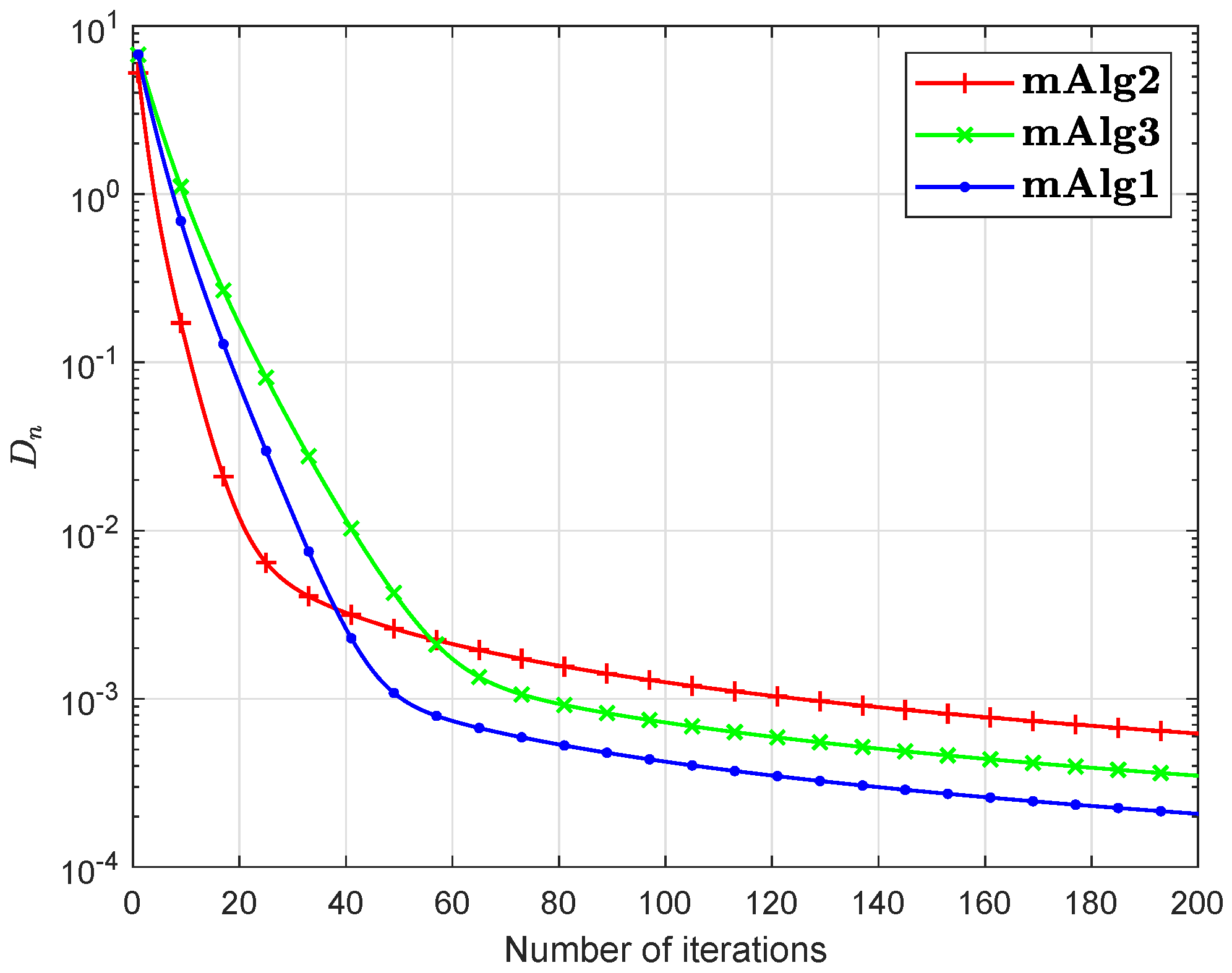
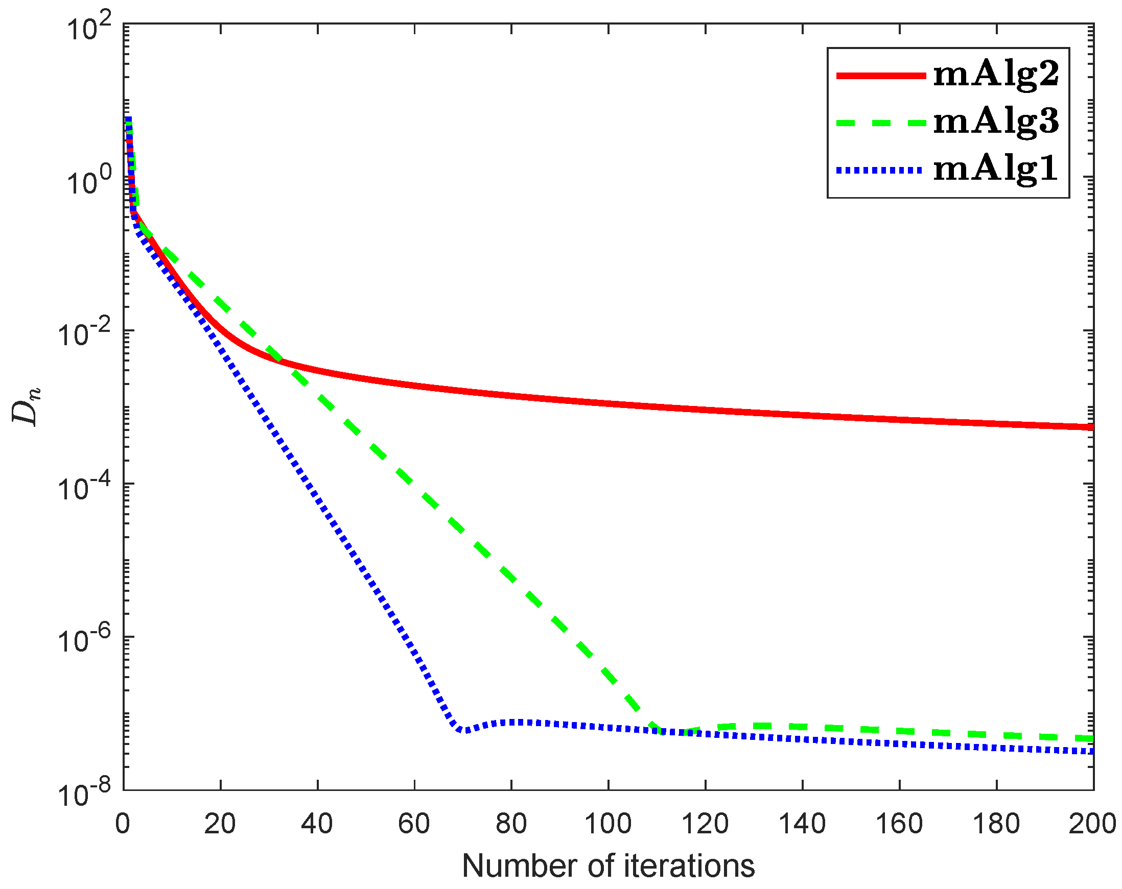
6. Numerical Illustrations

Numerical results are presented in this section to demonstrate the efficiency of our proposed method. The MATLAB codes were run in MATLAB version 9.5 (R2018b) on an Intel(R) Core(TM)i5-6200 CPU PC @ 2.30 GHz 2.40 GHz, RAM 4.00 GB.

Example 1.

Let there be m companies that manufacture the same product. Assume vector u of each item $u_i$ represents the quantity of the material produced by a company i. We consider that cost function P to be a declining affine function that relies on $\mu ={\sum }_{i=1}^m{u}_i$, i.e., $P_i\left(\mu \right)={\varphi }_i-{\psi }_{i}S,$ where ${\varphi }_i>0,$${\psi }_i>0.$ The formula for profit of every company i is taken as $F_i\left(u\right)=P_i\left(S\right)u_i-q_i\left(u_i\right),$ where $q_i\left(u_i\right)$ is the tax value and cost for developing item $u_i.$ Moreover, consider that ${\mathcal{C}}_i=[u_i^{min},u_i^{max}]$ is the set of actions related to each company $i,$ and the plan to figure out the model as $\mathcal{C}:={\mathcal{C}}_1\times {\mathcal{C}}_2\times \cdots \times {\mathcal{C}}_m.$ In addition, each member wants to achieve its peak turnover by a good level of production on the basis that the performance of other firms is an input parameter. The commonly used modelling methodology is based on the famous Nash equilibrium principle. A point $u^{*}\in \mathcal{C}={\mathcal{C}}_1\times {\mathcal{C}}_2\times \cdots \times {\mathcal{C}}_m$ is the level of equilibrium of the model if

$$F_i\left(u^{*}\right)\ge F_i\left(u^{*}\left[u_i\right]\right),\forall u_i\in {\mathcal{C}}_i,\forall i=1,2,\cdots ,m,$$

wile $u^{*}\left[u_i\right]$ is obtain from $u^{*}$ by letting ${\zeta }_i^{*}$ with $u_i.$ Furthermore, we consider $f(u,y):=\Delta (u,y)-\Delta (u,u)$ while $\Delta (u,y):=-{\sum }_{i=1}^m{F}_i\left(u\left[y_i\right]\right).$ An equilibrium level of the model is defined by

$$Find{u}^{*}\in \mathcal{C}:f(u^{*},z)\ge 0,\forall z\in \mathcal{C}.$$

Bifunction f converts into the following form (see [23]):

$$f(u,y)=\langle Pu+Qy+c,y-u\rangle$$

where $c\in {\mathcal{R}}^m$ and P, Q matrices of order $m.$ Matrix P is positive semidefinite, and matrix $Q-P$ is negative semidefinite with Lipschitz-type constants $c_1=c_2=\frac{1}{2}\parallel P-Q\parallel$ (see [23]) for details. $P,Q$ are taken randomly. (Two diagonal matrices randomly $A_1$ and $A_2$ take elements from $[0,2]$ and $[-2,0]$ respectively. Randomly $O_1=RandOrthMat\left(m\right)$ and $O_2=RandOrthMat\left(m\right)$ orthogonal matrices are generated. Then, a positive semidefinite matrix $B_1=O_1{A}_1{O}_1^T$ and a negative semidefinite matrix $B_2=O_2{A}_2{O}_2^T$ are achieved. Lastly, set $Q=B_1+B_1^T,$$S=B_2+B_2^T$ and $P=Q-S.$). The constraint set $C\subset {\mathcal{R}}^m$ be defined by

$$\mathcal{C}:=\{u\in {\mathcal{R}}^m:-10\le u_i\le 10\}.$$

Numerical explanations for the first 200 iterations of three methods are considered in Figure 1, Figure 2, Figure 3, Figure 4, Figure 5 and Figure 6 and

Table 1. Figure 1, Figure 2, Figure 3, Figure 4, Figure 5 and Figure 6 execution time required for first 200 iterations.

	Execution Time in Seconds
$\mathit{m}$	mAlg2	mAlg3	mAlg1
5	2.55846812	2.73622248	2.923849848
10	2.89823133	2.99853685	3.341848537
20	3.23847254	3.51835212	3.332562246
50	3.93645046	4.05462157	4.084188882
100	4.57837436	5.32873548	5.723835682
200	5.86241836	6.28194713	6.825465869

by letting initial points $u_0=u_{-1}={(1,1,\cdots ,1,1)}^T$. For Algorithm 3.2 (mAlg2) in [34]: $\chi =\frac{1}{4c_1}$ and ${\rho }_n=\frac{1}{100(n+2)}$; For Algorithm (mAlg3) in (60): ${\chi }_0=0.20$, $\mu =0.70$, ${\varrho }_n=\frac{1}{100(n+2)}$, ${\rho }_n=0.5(1-{\varrho }_n)$; For Algorithm 1 (mAlg1): ${\chi }_0=0.20$, $\mu =0.70$, $\varphi =0.60$, ${\varsigma }_n=\frac{1}{{(n+1)}^2}$, ${\varrho }_n=\frac{1}{100(n+2)}$ and ${\rho }_n=0.5(1-{\varrho }_n)$.

Example 2.

Assume that set $\mathcal{C}\subset L^2([0,1]$ is defined by

$$\mathcal{C}:=\{u\in L^2\left([0,1]\right):\parallel u\parallel \le 1\}.$$

Let us define an operator $\mathcal{L}:\mathcal{C}\to \mathcal{H}$, such that

$$\mathcal{L}\left(u\right)\left(t\right)={\int }_0^1\left[u\left(t\right)-H(t,s)f\left(u\right(s\left)\right)\right]ds+g\left(t\right),$$

where $H(t,s)=\frac{2ts{e}^{(t+s)}}{e\sqrt{e^2-1}},$$f\left(u\right)=cos\left(u\right)$ and $g\left(t\right)=\frac{2t{e}^t}{e\sqrt{e^2-1}}.$ In the above $\mathcal{H}=L^2\left([0,1]\right)$ is a Hilbert space with inner product $\langle u,y\rangle ={\int }_0^{1}u\left(t\right)y\left(t\right)dt,\forall u,y\in \mathcal{H}$ and induced norm is $\parallel u\parallel =\sqrt{{\int }_0^1{\left|u\left(t\right)\right|}^{2}dt}.$ Numerical explanations for the first 200 iterations of three methods are considered in Figure 7, Figure 8, Figure 9 and Figure 10 by letting initial points $u_0=u_{-1}={(1,1,\cdots ,1,1)}^T$. For Algorithm 3.2 (mAlg2) in [34]: $\chi =\frac{1}{3c_1}$ and ${\rho }_n=\frac{1}{100(n+2)}$; For Algorithm (mAlg3) in (60): ${\chi }_0=0.50$, $\mu =0.50$, ${\varrho }_n=\frac{1}{100(n+2)}$, ${\rho }_n=0.7(1-{\varrho }_n)$; For Algorithm 1 (mAlg1): ${\chi }_0=0.50$, $\mu =0.50$, $\varphi =0.70$, ${\varsigma }_n=\frac{1}{{(n+1)}^2}$, ${\varrho }_n=\frac{1}{100(n+2)}$ and ${\rho }_n=0.7(1-{\varrho }_n)$.

7. Conclusions

We studied a Mann-type extragradient-like scheme for determining the numerical solution of equilibrium problem involving pseudomonotone function and also prove a strong convergent theorem. Computational conclusions were established to illustrate the computational performance of our algorithms relative to other approaches. Such computational experiments showed that the inertial effect increases the efficacy of the iterative method in this sense.

References

1. Fan, K. A Minimax Inequality and Applications, Inequalities III; Shisha, O., Ed.; Academic Press: New York, NY, USA, 1972. [Google Scholar]
2. Muu, L.; Oettli, W. Convergence of an adaptive penalty scheme for finding constrained equilibria. Nonlinear Anal. Theory Methods Appl. 1992, 18, 1159–1166. [Google Scholar] [CrossRef]
3. Blum, E. From optimization and variational inequalities to equilibrium problems. Math. Stud. 1994, 63, 123–145. [Google Scholar]
4. Bigi, G.; Castellani, M.; Pappalardo, M.; Passacantando, M. Existence and solution methods for equilibria. Eur. J. Oper. Res. 2013, 227, 1–11. [Google Scholar] [CrossRef] [Green Version]
5. Antipin, A. Equilibrium programming: Proximal methods. Comput. Math. Math. Phys. 1997, 37, 1285–1296. [Google Scholar]
6. Giannessi, F.; Maugeri, A.; Pardalos, P.M. Equilibrium Problems: Nonsmooth Optimization and Variational Inequality Models; Kluwer Academic Publisher: Dordrecht, The Netherlands, 2006; Volume 58. [Google Scholar]
7. Dafermos, S. Traffic Equilibrium and Variational Inequalities. Transp. Sci. 1980, 14, 42–54. [Google Scholar] [CrossRef] [Green Version]
8. ur Rehman, H.; Kumam, P.; Cho, Y.J.; Yordsorn, P. Weak convergence of explicit extragradient algorithms for solving equilibirum problems. J. Inequalities Appl. 2019, 2019. [Google Scholar] [CrossRef]
9. Ur Rehman, H.; Pakkaranang, N.; Kumam, P.; Cho, Y.J. Modified subgradient extragradient method for a family of pseudomonotone equilibrium problems in real a Hilbert space. J. Nonlinear Convex Anal. 2020, 21, 2011–2025. [Google Scholar]
10. Ur Rehman, H.; Kumam, P.; Dong, Q.L.; Cho, Y.J. A modified self-adaptive extragradient method for pseudomonotone equilibrium problem in a real Hilbert space with applications. Math. Methods Appl. Sci. 2020, 44, 3527–3547. [Google Scholar] [CrossRef]
11. Ur Rehman, H.; Kumam, P.; Sitthithakerngkiet, K. Viscosity-type method for solving pseudomonotone equilibrium problems in a real Hilbert space with applications. AIMS Math. 2021, 6, 1538–1560. [Google Scholar] [CrossRef]
12. Ur Rehman, H.; Kumam, P.; Gibali, A.; Kumam, W. Convergence analysis of a general inertial projection-type method for solving pseudomonotone equilibrium problems with applications. J. Inequalities Appl. 2021, 2021. [Google Scholar] [CrossRef]
13. Rehman, H.U.; Kumam, P.; Dong, Q.L.; Peng, Y.; Deebani, W. A new Popov’s subgradient extragradient method for two classes of equilibrium programming in a real Hilbert space. Optimization 2020, 1–36. [Google Scholar] [CrossRef]
14. Ur Rehman, H.; Kumam, P.; Shutaywi, M.; Alreshidi, N.A.; Kumam, W. Inertial Optimization Based Two-Step Methods for Solving Equilibrium Problems with Applications in Variational Inequality Problems and Growth Control Equilibrium Models. Energies 2020, 13, 3292. [Google Scholar] [CrossRef]
15. Ferris, M.C.; Pang, J.S. Engineering and Economic Applications of Complementarity Problems. Siam Rev. 1997, 39, 669–713. [Google Scholar] [CrossRef] [Green Version]
16. Ur Rehman, H.; Kumam, P.; Cho, Y.J.; Suleiman, Y.I.; Kumam, W. Modified Popov’s explicit iterative algorithms for solving pseudomonotone equilibrium problems. Optim. Methods Softw. 2020, 36, 82–113. [Google Scholar] [CrossRef]
17. Ur Rehman, H.; Kumam, P.; Abubakar, A.B.; Cho, Y.J. The extragradient algorithm with inertial effects extended to equilibrium problems. Comput. Appl. Math. 2020, 39. [Google Scholar] [CrossRef]
18. Ur Rehman, H.; Pakkaranang, N.; Hussain, A.; Wairojjana, N. A modified extra-gradient method for a family of strongly pseudomonotone equilibrium problems in real Hilbert spaces. J. Math. Comput. Sci. 2020, 22, 38–48. [Google Scholar] [CrossRef]
19. Wairojjana, N.; ur Rehman, H.; Argyros, I.K.; Pakkaranang, N. An Accelerated Extragradient Method for Solving Pseudomonotone Equilibrium Problems with Applications. Axioms 2020, 9, 99. [Google Scholar] [CrossRef]
20. Wairojjana, N.; ur Rehman, H.; la Sen, M.D.; Pakkaranang, N. A General Inertial Projection-Type Algorithm for Solving Equilibrium Problem in Hilbert Spaces with Applications in Fixed-Point Problems. Axioms 2020, 9, 101. [Google Scholar] [CrossRef]
21. Wairojjana, N.; Pakkaranang, N.; Ur Rehman, H.; Pholasa, N.; Khanpanuk, T. Strong Convergence of Extragradient-Type Method to Solve Pseudomonotone Variational Inequalities Problems. Axioms 2020, 9, 115. [Google Scholar] [CrossRef]
22. Wairojjana, N.; Younis, M.; Ur Rehman, H.; Pakkaranang, N.; Pholasa, N. Modified Viscosity Subgradient Extragradient-Like Algorithms for Solving Monotone Variational Inequalities Problems. Axioms 2020, 9, 118. [Google Scholar] [CrossRef]
23. Tran, D.Q.; Dung, M.L.; Nguyen, V.H. Extragradient algorithms extended to equilibrium problems. Optimization 2008, 57, 749–776. [Google Scholar] [CrossRef]
24. Korpelevich, G. The extragradient method for finding saddle points and other problems. Matecon 1976, 12, 747–756. [Google Scholar]
25. Hieu, D.V.; Quy, P.K.; Vy, L.V. Explicit iterative algorithms for solving equilibrium problems. Calcolo 2019, 56. [Google Scholar] [CrossRef]
26. Polyak, B. Some methods of speeding up the convergence of iteration methods. USSR Comput. Math. Math. Phys. 1964, 4, 1–17. [Google Scholar] [CrossRef]
27. Beck, A.; Teboulle, M. A Fast Iterative Shrinkage-Thresholding Algorithm for Linear Inverse Problems. SIAM J. Imaging Sci. 2009, 2, 183–202. [Google Scholar] [CrossRef] [Green Version]
28. Hung, P.G.; Muu, L.D. The Tikhonov regularization extended to equilibrium problems involving pseudomonotone bifunctions. Nonlinear Anal. Theory Methods Appl. 2011, 74, 6121–6129. [Google Scholar] [CrossRef]
29. Konnov, I. Application of the Proximal Point Method to Nonmonotone Equilibrium Problems. J. Optim. Theory Appl. 2003, 119, 317–333. [Google Scholar] [CrossRef]
30. Moudafi, A. Proximal point algorithm extended to equilibrium problems. J. Nat. Geom. 1999, 15, 91–100. [Google Scholar]
31. Oliveira, P.; Santos, P.; Silva, A. A Tikhonov-type regularization for equilibrium problems in Hilbert spaces. J. Math. Anal. Appl. 2013, 401, 336–342. [Google Scholar] [CrossRef]
32. Mann, W.R. Mean value methods in iteration. Proc. Am. Math. Soc. 1953, 4, 506. [Google Scholar] [CrossRef]
33. Censor, Y.; Gibali, A.; Reich, S. The Subgradient Extragradient Method for Solving Variational Inequalities in Hilbert Space. J. Optim. Theory Appl. 2010, 148, 318–335. [Google Scholar] [CrossRef] [Green Version]
34. Hieu, D.V. Halpern subgradient extragradient method extended to equilibrium problems. Rev. Real Acad. Cienc. Exactas FÍSicas Nat. Ser. Matemíticas 2016, 111, 823–840. [Google Scholar] [CrossRef]
35. Bianchi, M.; Schaible, S. Generalized monotone bifunctions and equilibrium problems. J. Optim. Theory Appl. 1996, 90, 31–43. [Google Scholar] [CrossRef]
36. Mastroeni, G. On Auxiliary Principle for Equilibrium Problems. In Nonconvex Optimization and Its Applications; Springer: New York, NY, USA, 2003; pp. 289–298. [Google Scholar] [CrossRef]
37. Tiel, J.V. Convex Analysis: An Introductory Text, 1st ed.; Wiley: New York, NY, USA, 1984. [Google Scholar]
38. Kreyszig, E. Introductory Functional Analysis with Applications, 1st ed.; Wiley: New York, NY, USA, 1989. [Google Scholar]
39. Xu, H.K. Another control condition in an iterative method for nonexpansive mappings. Bull. Aust. Math. Soc. 2002, 65, 109–113. [Google Scholar] [CrossRef] [Green Version]
40. Maingé, P.E. Strong Convergence of Projected Subgradient Methods for Nonsmooth and Nonstrictly Convex Minimization. Set Valued Anal. 2008, 16, 899–912. [Google Scholar] [CrossRef]
41. Bauschke, H.H.; Combettes, P.L. Convex Analysis and Monotone Operator Theory in Hilbert Spaces, 2nd ed.; CMS Books in Mathematics; Springer International Publishing: New York, NY, USA, 2017. [Google Scholar]
42. Browder, F.; Petryshyn, W. Construction of fixed points of nonlinear mappings in Hilbert space. J. Math. Anal. Appl. 1967, 20, 197–228. [Google Scholar] [CrossRef] [Green Version]
43. Wang, S.; Zhang, Y.; Ping, P.; Cho, Y.; Guo, H. New extragradient methods with non-convex combination for pseudomonotone equilibrium problems with applications in Hilbert spaces. Filomat 2019, 33, 1677–1693. [Google Scholar] [CrossRef] [Green Version]
44. Stampacchia, G. Formes bilinéaires coercitives sur les ensembles convexes. Comptes Rendus Hebd. Seances Acad. Sci. 1964, 258, 4413. [Google Scholar]
45. Konnov, I.V. On systems of variational inequalities. Russ. Math. C/C Izv. Vyss. Uchebnye Zaved. Mat. 1997, 41, 77–86. [Google Scholar]
Figure 1. Algorithm 1 compared to Algorithm (60) and Algorithm 3.2 in [34] for R 5 .
Axioms 10 00076 g001
Figure 2. Algorithm 1 compared to Algorithm (60) and Algorithm 3.2 in [34] for R 10 .
Axioms 10 00076 g002
Figure 3. Algorithm 1 compared to Algorithm (60) and Algorithm 3.2 in [34] for R 20 .
Axioms 10 00076 g003
Figure 4. Algorithm 1 compared to Algorithm (60) and Algorithm 3.2 in [34] for R 50 .
Axioms 10 00076 g004
Figure 5. Algorithm 1 compared to Algorithm (60) and Algorithm 3.2 in [34] for R 100 .
Axioms 10 00076 g005
Figure 6. Algorithm 1 compared to Algorithm (60) and Algorithm 3.2 in [34] for R 200 .
Axioms 10 00076 g006
Figure 7. Algorithm 1 compared to Algorithm (60) and Algorithm 3.2 in [34] for u 0 = 1 + t + 2 t 2 .
Axioms 10 00076 g007
Figure 8. Algorithm 1 compared to Algorithm (60) and Algorithm 3.2 in [34] for u 0 = 1 + 2 t + 3 e t .
Axioms 10 00076 g008
Figure 9. Algorithm 1 compared to Algorithm (60) and Algorithm 3.2 in [34] for u 0 = 1 + 2 t + sin ( t ) .
Axioms 10 00076 g009
Figure 10. Algorithm 1 compared to Algorithm (60) and Algorithm 3.2 in [34] for u 0 = 1 + 3 t 2 + cos ( t ) .
Axioms 10 00076 g010