
Applications of Coupled Fixed Points for Multivalued Maps in the Equilibrium in Duopoly Markets and in Aquatic Ecosystems

 ,
,  , , and
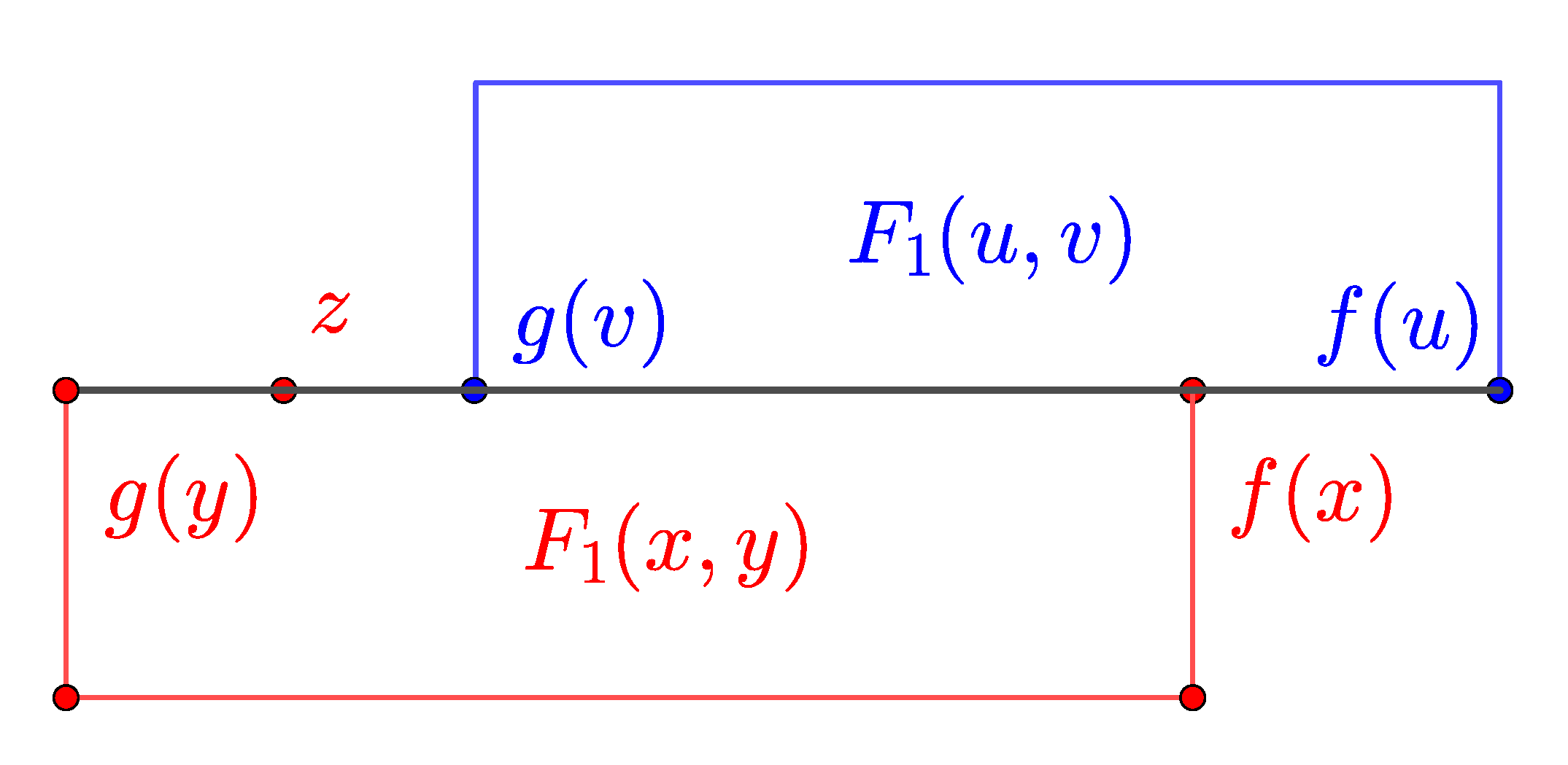
Abstract
1. Introduction
2. Preliminaries
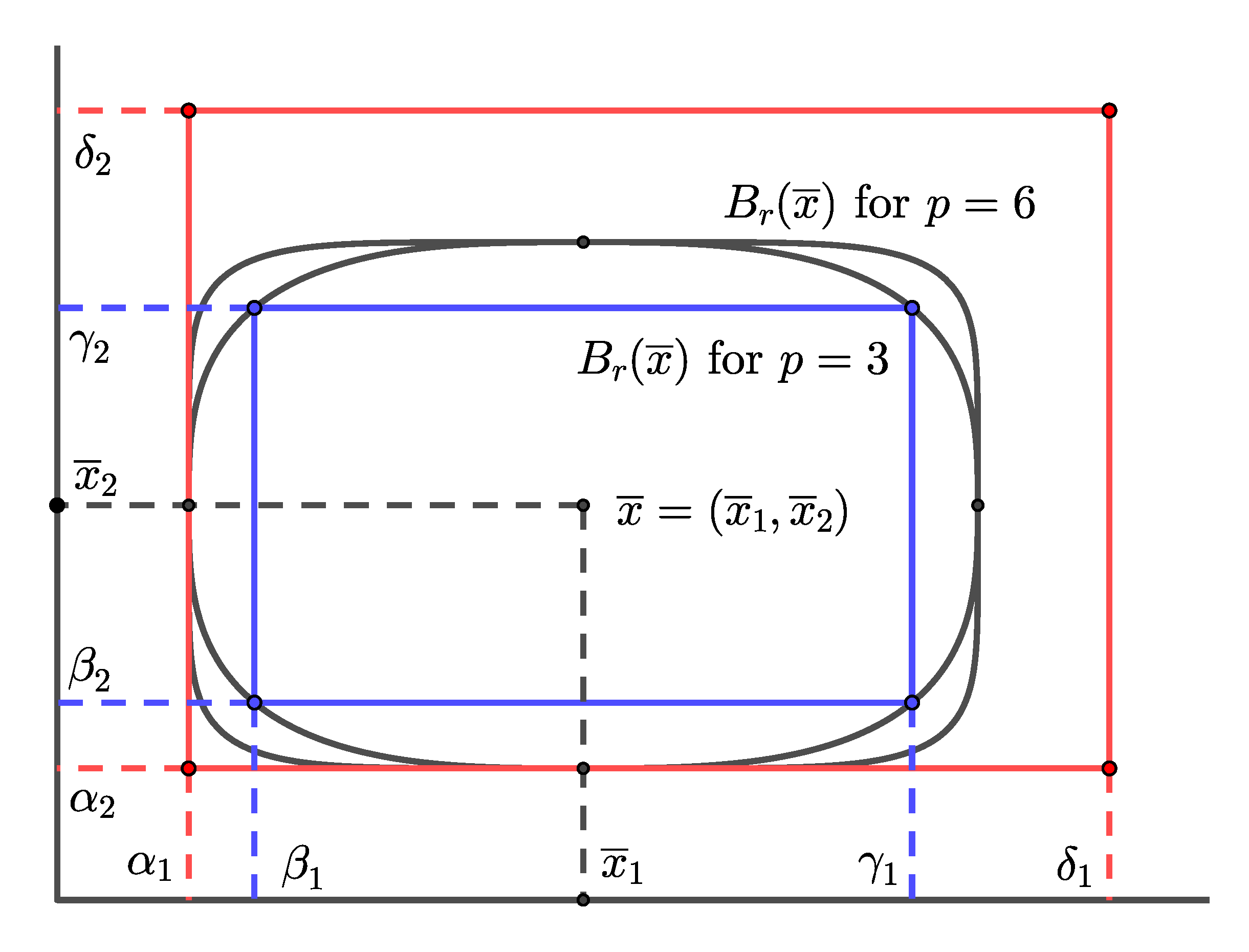
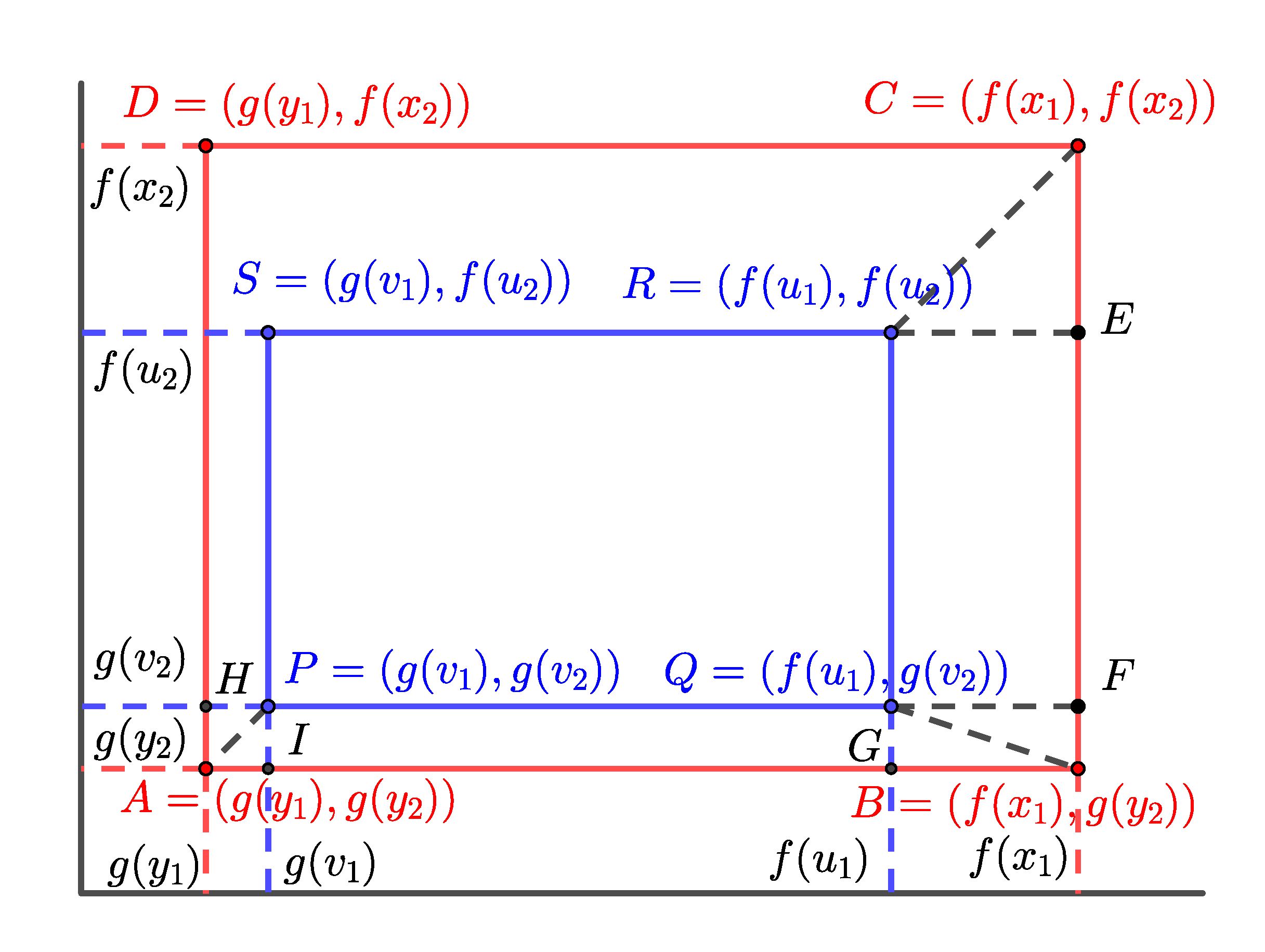
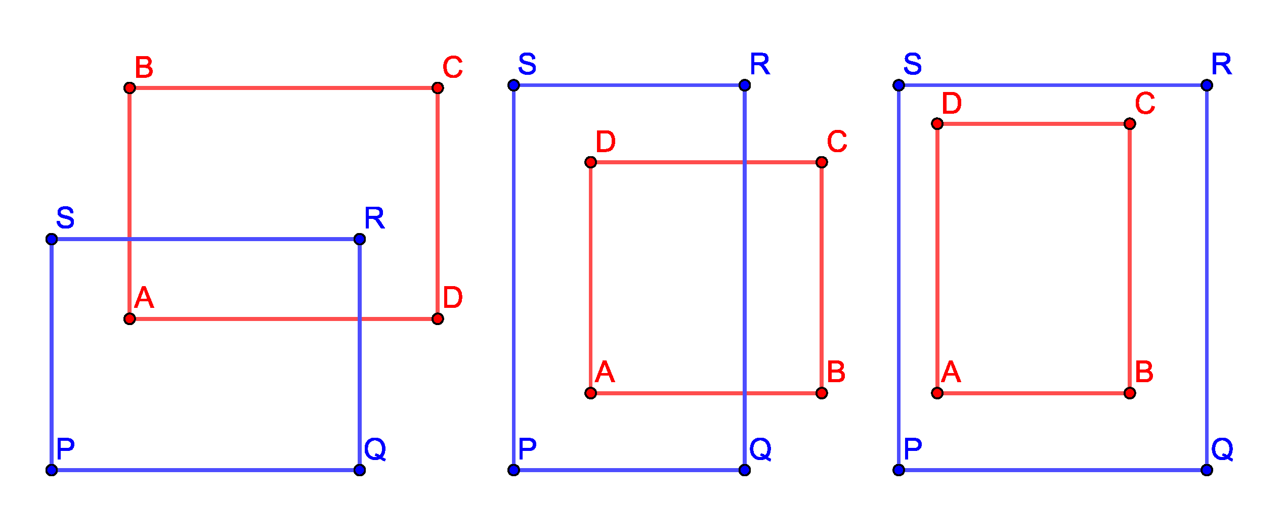
3. Main Results
4. Examples and Applications
4.1. Examples
4.2. Examples for the Existence of an Equilibrium in Oligopoly (Duopoly) Markets
4.3. Example for the Existence of an Equilibrium in Ecology
Author Contributions
Funding
Institutional Review Board Statement
Informed Consent Statement
Data Availability Statement
Acknowledgments
Conflicts of Interest
References
- Nadler, S.B. Multi–Valued Contraction Mappings. Pac. J. Math. 1969, 30, 475–488. [Google Scholar] [CrossRef]
- Dontchev, A.; Hager, W. An inverse mapping theorem for set-valued maps. Proc. Am. Math. Soc. 1994, 121, 481–489. [Google Scholar] [CrossRef]
- Ahmad, W.; Sarwar, M.; Abdeljawad, T.; Rahmat, G. Multi–Valued Versions of Nadler, Banach, Branciari and Reich Fixed Point Theorems in Double Controlled Metric Type Spaces with Applications. AIMS Math. 2021, 6, 477–499. [Google Scholar] [CrossRef]
- Alsaedi, A.; Broom, A.; Ntouyas, S.K.; Ahmad, B. Nonlocal Fractional Boundary Value Problems Involving Mixed Right and Left Fractional Derivatives and Integrals. Axioms 2020, 9, 50. [Google Scholar] [CrossRef]
- Chen, L.; Yang, N.; Zhou, J. Common Attractive Points of Generalized Hybrid Multi–Valued Mappings and Applications. Mathematics 2020, 8, 1307. [Google Scholar] [CrossRef]
- Shoaib, M.; Sarwar, M.; Kumam, P. Multi-Valued Fixed Point Theorem via F–Contraction of Nadler Type and Application to Functional and Integral Equations. Bol. Soc. Paran. Mat. 2021, 39, 83–95. [Google Scholar] [CrossRef]
- Bhaskar, T.G.; Lakshmikantham, N. Fixed Point Theorems in Partially Ordered Metric Spaces and Applications. Nonlinear Anal. 2006, 65, 1379–1393. [Google Scholar] [CrossRef]
- George, R.; Mitrović, Z.D.; Radenovixcx, S. On Some Coupled Fixed Points of Generalized T–Contraction Mappings in a bv(s)–Metric Space and Its Application. Axioms 2020, 9, 129. [Google Scholar] [CrossRef]
- Kim, K.S. A Constructive Scheme for a Common Coupled Fixed Point Problems in Hilbert Space. Mathematics 2020, 8, 1717. [Google Scholar] [CrossRef]
- Kishore, G.; Rao, B.S.; Radenović, S.; Huang, H.P. Caristi Type Cyclic Contraction and Coupled Fixed Point Results in Bipolar Metric Spaces. Sahand Commun. Math. Anal. 2020, 17, 1–22. [Google Scholar] [CrossRef]
- Shateri, T. Coupled fixed points theorems for non-linear contractions in partially ordered modular spaces. Int. J. Nonlinear Anal. Appl. 2020, 11, 133–147. [Google Scholar] [CrossRef]
- Kirk, W.; Srinivasan, P.; Veeramani, P. Fixed points for mappings satisfying cyclical contractive conditions. Fixed Point Theory 2003, 4, 79–189. [Google Scholar]
- Eldred, A.; Veeramani, P. Existence and convergence of best proximity points. J. Math. Anal. Appl. 2006, 323, 1001–1006. [Google Scholar] [CrossRef]
- Abdeljawad, T.; Ullah, K.; Ahmad, J.; Sen, M.D.L.; Ulhaq, A. Approximation of Fixed Points and Best Proximity Points of Relatively Nonexpansive Mappings. J. Math. 2020, 2020, 8821553. [Google Scholar] [CrossRef]
- Debnath, P.; Srivastava, H.M. Global Optimization and Common Best Proximity Points for Some Multivalued Contractive Pairs of Mappings. Axioms 2020, 9, 102. [Google Scholar] [CrossRef]
- Mishra, L.N.; Dewangan, V.; Mishra, V.N.; Karateke, S. Best proximity points of admissible almost generalized weakly contractive mappings with rational expressions on b–metric spaces. J. Math. Comput. Sci. 2021, 22, 97–109. [Google Scholar] [CrossRef]
- Pant, R.; Shukla, R.; Rakocevic, V. Approximating best proximity points for Reich type non-self nonexpansive mappings. Rev. R. Acad. Cienc. Exactas Fìs. Nat. Ser. A Mat. RACSAM 2020, 114, 197. [Google Scholar] [CrossRef]
- Dzhabarova, Y.; Kabaivanov, S.; Ruseva, M.; Zlatanov, B. Existence, Uniqueness and Stability of Market Equilibrium in Oligopoly Markets. Adm. Sci. 2020, 10, 70. [Google Scholar] [CrossRef]
- Kabaivanov, S.; Zlatanov, B. A variational principle, coupled fixed points and market equilibrium. Nonlinear Anal. Model. Control. 2021, 26, 169–185. [Google Scholar] [CrossRef]
- Zhang, X. Fixed Point Theorems of Multivalued Monotone Mappings in Ordered Metric Spaces. Appl. Math. Lett. 2010, 23, 235–240. [Google Scholar] [CrossRef][Green Version]
- Cournot, A.A. Researches into the Mathematical Principles of the Theory of Wealth, Translation ed.; Macmillan: New York, NY, USA, 1897. [Google Scholar]
- Friedman, J.W. Oligopoly Theory; Cambradge University Press: Cambradge, UK, 2007. [Google Scholar]
- Matsumoto, A.; Szidarovszky, F. Dynamic Oligopolies with Time Delays; Springer Nature Singapore Pte Ltd.: Singapore, 2018. [Google Scholar]
- Okuguchi, K.; Szidarovszky, F. The Theory of Oligopoly with Multi–Product Firms; Springer: Berlin/Heidelberg, Germany, 1990. [Google Scholar]
- Smith, A. A Mathematical Introduction to Economics; Basil Blackwell Limited: Oxford, UK, 1982. [Google Scholar]
- Empain, A.M. A posteriori detection of heavy metal pollution of aquatic habitats. In Methods in Bryology. Proc. Bryol. Method. Workshop, Mainz; Glime, J.M., Ed.; Hattori Bot Lab.: Nichinan, Japan, 1988; pp. 213–220. [Google Scholar]
- Gecheva, G.; Yurukova, L. Water pollutant monitoring with aquatic bryophytes: A review. Environ. Chem. Lett. 2014, 12, 49–61. [Google Scholar] [CrossRef]
- Gecheva, G.; Yancheva, V.; Velcheva, I.; Georgieva, E.; Stoyanova, S.; Arnaudova, D.; Stefanova, V.; Georgieva, D.; Genina, V.; Todorova, B.; et al. Integrated Monitoring with Moss-Bag and Mussel Transplants in Reservoirs. Water 2020, 12, 1800. [Google Scholar] [CrossRef]


Publisher’s Note: MDPI stays neutral with regard to jurisdictional claims in published maps and institutional affiliations. |
© 2021 by the authors. Licensee MDPI, Basel, Switzerland. This article is an open access article distributed under the terms and conditions of the Creative Commons Attribution (CC BY) license (http://creativecommons.org/licenses/by/4.0/).
Share and Cite
Gecheva, G.; Hristov, M.; Nedelcheva, D.; Ruseva, M.; Zlatanov, B. Applications of Coupled Fixed Points for Multivalued Maps in the Equilibrium in Duopoly Markets and in Aquatic Ecosystems. Axioms 2021, 10, 44. https://doi.org/10.3390/axioms10020044
Gecheva G, Hristov M, Nedelcheva D, Ruseva M, Zlatanov B. Applications of Coupled Fixed Points for Multivalued Maps in the Equilibrium in Duopoly Markets and in Aquatic Ecosystems. Axioms. 2021; 10(2):44. https://doi.org/10.3390/axioms10020044
Chicago/Turabian StyleGecheva, Gana, Miroslav Hristov, Diana Nedelcheva, Margarita Ruseva, and Boyan Zlatanov. 2021. "Applications of Coupled Fixed Points for Multivalued Maps in the Equilibrium in Duopoly Markets and in Aquatic Ecosystems" Axioms 10, no. 2: 44. https://doi.org/10.3390/axioms10020044
APA StyleGecheva, G., Hristov, M., Nedelcheva, D., Ruseva, M., & Zlatanov, B. (2021). Applications of Coupled Fixed Points for Multivalued Maps in the Equilibrium in Duopoly Markets and in Aquatic Ecosystems. Axioms, 10(2), 44. https://doi.org/10.3390/axioms10020044