Analysis of the Transient Behaviour in the Numerical Solution of Volterra Integral Equations

Abstract

In this paper, the asymptotic behaviour of the numerical solution to the Volterra integral equations is studied. In particular, a technique based on an appropriate splitting of the kernel is introduced, which allows one to obtain vanishing asymptotic (transient) behaviour in the numerical solution, consistently with the properties of the analytical solution, without having to operate restrictions on the integration steplength.

1. Introduction

Volterra integral equations (VIEs) of the type

$$x\left(t\right)=g\left(t\right)+{\int }_0^{t}K(t,s)x\left(s\right)ds,t\in [0,+\infty ),$$

(1)

and their discrete version,

$$x\left(t\right)=g\left(t\right)+\sum _{s=0}^{t}K(t,s)x\left(s\right),t=1,2,\dots ,x\left(0\right)\mathrm{given},$$

(2)

are significative mathematical models for representing real-life problems involving feedback and control [1,2]. The analysis of their dynamics allows one to describe the phenomena they represent. In [3], the two equations were analysed in the unifying notation of time scales, and some results were obtained under linear perturbation of the kernel. Here, we revise this approach to obtain results on classes of linear discrete equations whose kernel can be split into a well-behaving part (the unperturbed kernel) plus a term that acts as a perturbation. The implications for numerical methods are, in general, not straightforward and pass through some restrictions on the step length. Nevertheless, here, we overcome this problem and obtain some results on the stability of numerical methods for VIEs.

For Equations (1) and (2), we assume that $x\left(t\right)={\left(x_1\left(t\right),\dots ,x_d\left(t\right)\right)}^T\in {\mathbb{R}}^d,$ $g\left(t\right)={\left(g_1\left(t\right),\dots ,g_d\left(t\right)\right)}^T\in {\mathbb{R}}^d,$ and $K(t,s)={\left(K_{ij}(t,s)\right)}_{i,j=1,\dots ,d}$ is a $d\times d$ matrix.

The paper is organised as follows. In Section 2, we introduce the split kernel for Equation (2) and, using a new formulation of Theorem 2 in [3], we provide sufficient conditions for the above-mentioned splitting that imply that the solution vanishes. In Section 3, we propose a reformulation of the $(\rho ,\sigma )$ methods for (1) as discrete Volterra equations and exploit the theory developed in the previous section in order to investigate its numerical stability properties. In Section 4, some applications are described and analysed through the tools developed in Section 2 and Section 3, for which we obtain new and more general results on the asymptotic behaviour for the numerical solutions of both linear and nonlinear equations. In Section 5, some numerical examples are reported.

2. Asymptotics for Discrete Equations

Consider the discrete Volterra Equation (2) with $K(t,s)=P(t,s)+Q(t,s),$ where P and Q are $d\times d$ matrices. Let $r_Q(t,s)$ be the resolvent kernel associated with $Q(t,s),$ which is defined as the solution of the equation:

$$r_Q(t,s)=Q(t,s)+\sum _{l=s+1}^t{r}_Q(t,l)Q(l,s).$$

(3)

The following theorem, which we proved in [3], represents the starting point of our investigation.

Theorem 1.

Assume that for Equation (2) with $K(t,s)=P(t,s)+Q(t,s),$ $s=0,\dots ,t$, it holds that:

(i) 

${\sum }_{s=0}^n\parallel r_Q(t,s)\parallel \le R,$$t\ge 0,$

(ii) 

${lim}_{t\to \infty }\parallel r_Q(t,s)\parallel =0,$ for any fixed $s\ge 0,$

(iii) 

${lim}_{t\to \infty }{\sum }_{s=0}^t\parallel P(t,s)\parallel =0.$

Then, if ${lim}_{t\to \infty }g\left(t\right)=0,$

$$\underset{t\to \infty }{lim}x\left(t\right)=0.$$

This theorem is particularly interesting when the matrix P in the splitting of kernel K is such that $P(t,s)=0$ for $s=M+1,\dots ,t-N-1,$ with M and N positive constants and $t\ge N+M+1.$ Then, Equation (2) can be rewritten as

$$x\left(t\right)=g\left(t\right)+\sum _{s=0}^{M}P(t,s)x\left(s\right)+\sum _{s=0}^{t}Q(t,s)x\left(s\right)+\sum _{s=t-N}^{t}P(t,s)x\left(s\right),$$

(4)

and the following result holds. Here and in the following, the limit of matrices is intended element-wise.

Theorem 2.

Consider Equation (4), and assume that:

(1) 

${lim}_{t\to \infty }P(t,s)=0,$ for $s=0,\dots ,M,$ and ${lim}_{t\to \infty }P(t,t)=0.$

(2) 

${\sum }_{s=0}^t\parallel Q(t,s)\parallel \le \alpha <1,$${lim}_{t\to \infty }Q(t,s)=0,$ for any fixed $s\ge 0.$

If there exists a constant $G>0$ such that $\parallel g\left(t\right)\parallel \le G,$ then

$$\parallel x\left(t\right)\parallel \le X,withX>0,$$

and if ${lim}_{t\to \infty }g\left(t\right)=0,$ then

$$\underset{t\to \infty }{lim}x\left(t\right)=0.$$

Proof. 

Assumption $\left(1\right)$ implies (iii) of Theorem 1 and, applying a well-known result (see, for example, [2] (Section 6) and [4]), for assumption (2), we have that (i) and (ii) hold. □

The case ${lim}_{t\to \infty }P(t,s)=P_{\infty }\left(s\right)\ne 0$ and ${lim}_{t\to \infty }g\left(t\right)=g_{\infty }\ne 0$ can be treated by the same technique if it is known that ${\sum }_{s=0}^{t}Q(t,s)\to E_{\infty }\ne I,$ for $t\to \infty$ (I is the $d\times d$ identity matrix). In this case, we have the following corollary.

Corollary 1.

Assume that, for Equation (4), there exists $M>0$ such that

(1) 

${lim}_{t\to \infty }P(t,s)=P_{\infty }\left(s\right),$ for $j=0,\dots ,M,$ and ${lim}_{t\to \infty }P(t,t)=0;$

(2) 

${\sum }_{s=0}^t\parallel Q(t,s)\parallel \le \alpha <1,$${lim}_{t\to \infty }Q(t,s)=0,$ for $s=0,\dots ,t;$

(3) 

${lim}_{t\to \infty }{\sum }_{s=0}^{t}Q(t,s)=E_{\infty }\ne I.$

If ${lim}_{t\to \infty }g\left(t\right)=g_{\infty },$ then

$$\underset{t\to \infty }{lim}x\left(t\right)={(I-E_{\infty })}^{-1}\left(g_{\infty }+\sum _{s=0}^M{P}_{\infty }\left(s\right)x\left(s\right)\right).$$

Proof. 

Set $x_{\infty }=(I-E_{\infty }^{-1})\left(g_{\infty }+{\sum }_{s=0}^M{P}_{\infty }\left(s\right)x\left(s\right)\right).$ A manipulation of (4) gives

$$\overline{x}\left(t\right)=\overline{g}\left(t\right)+\sum _{s=0}^t\overline{Q}(t,s)\overline{x}\left(s\right)+\sum _{s=t-N}^t\overline{P}(t,s)\overline{x}\left(s\right),$$

with $\overline{x}\left(t\right)=x\left(t\right)-x_{\infty },$$\overline{P}(t,s)=0,$ for $s=0,\dots ,M,$ $\overline{P}(t,s)=P(t,s),$ for $s=t-N,\dots ,t,$ $\overline{Q}(t,s)=Q(t,s),$ and

$$\overline{g}\left(t\right)=g\left(t\right)-g_{\infty }+\left(\sum _{s=0}^{t}Q(t,s)-E_{\infty }\right)x_{\infty }+\sum _{s=0}^M(P(t,s)-P_{\infty }\left(s\right))x_{\infty }+\sum _{s=t-N}^{t}P(t,s)x_{\infty }.$$

$\overline{P},$ $\overline{Q}$, and $\overline{g}$ play the roles of $P,$ Q, and g in (4). Recalling Theorem 1, all of the assumptions are satisfied, which implies that ${lim}_{t\to +\infty }\overline{x}\left(t\right)=0,$ and then ${lim}_{t\to +\infty }x\left(t\right)=x_{\infty }.$ □

3. Background Material on $(\mathbf{\rho },\mathbf{\sigma })$ Methods

The analysis carried out in the previous section can be effectively applied to $(\rho ,\sigma )$ methods for the systems of VIEs:

$$y\left(t\right)=f\left(t\right)+{\int }_0^{t}k(t,s)y\left(s\right)ds,t\in [0,+\infty ).$$

(5)

Here, we consider the numerical solution to (5) obtained by the $(\rho ,\sigma )$ methods with Gregory convolution weights (see, for example, [5,6,7]):

$$y_n=f\left(t_n\right)+h\sum _{j=0}^{n_0-1}{w}_{nj}k(t_n,t_j)y_j+h\sum _{j=n_0}^n{\omega }_{n-j}k(t_n,t_j)y_j,$$

(6)

$n=n_0,n_0+1,\dots ,$ where $y_n\simeq y\left(t_n\right),$ with $t_n=nh$ for $n=0,1,\dots ,$ $h>0$ is the step size and $w_{nj},$ ${\omega }_j$ are the weights. We assume that the weights are non-negative and that $y_0=f\left(0\right),y_1\dots ,y_{n_0-1},$ $n_0\ge 1,$ are given starting values.

The weights $w_{nj},$ $n=0,1,\dots ,$$j=0,1,\dots ,n_0-1$ are called the starting weights and satisfy (see [5]):

$$\underset{n\ge 0}{sup}{w}_{nj}\le W<+\infty ,j=0,\dots ,n_0-1,\mathrm{and}\underset{n\to \infty }{lim}{w}_{nj}={\overline{w}}_j.$$

(7)

Moreover, we want to underline some properties of the Gregory convolution weights, ${\omega }_n$ (see, for example [5,7]), which will be useful in the subsequent sections:

$$\underset{n}{sup}{\omega }_n=\mathsf{\Omega }<+\infty ,$$

(8)

$${\omega }_i=1,\mathrm{for} i\ge n_0.$$

(9)

From now on, we assume that h satisfies

$$det(I-h{\omega }_{0}k(t_n,t_n))\ne 0,$$

(10)

where I is the identity matrix of size d.

Choose $n^{*}>n_0$ and let

$$P(n,j)=\left\{\begin{array}{cc}0,\hfill & j=0,\dots ,n_0-1,\hfill \\ hk(t_n,t_j),\hfill & j=n_0,\dots ,n^{*}-1,\hfill \\ h{\omega }_{n-j}k(t_n,t_j),\hfill & j=n-n_0+1,\dots ,n,\hfill \end{array}\right.$$

and

$$Q(n,j)=\left\{\begin{array}{cc}0,\hfill & j=0,\dots ,n^{*}-1,j=n-n_0+1,\dots ,n,\hfill \\ hk(t_n,t_j),\hfill & j=n^{*},\dots ,n-n_0.\hfill \end{array}\right.$$

The $(\rho ,\sigma )$ method (6) can be written, for $n=n^{*}+n_0,n^{*}+n_0+1,\dots ,$ as follows:

$$y_n=g\left(n\right)+\sum _{j=n_0}^{n^{*}-1}P(n,j)y_j+\sum _{j=n^{*}}^{n-n_0}Q(n,j)y_j+\sum _{j=n-n_0+1}^{n}P(n,j)y_j,$$

(11)

with $g\left(n\right)=f\left(t_n\right)+h{\sum }_{j=0}^{n_0-1}{w}_{nj}k(t_n,t_j)y_j.$ This alternative formulation of the method in terms of matrices P and Q allows us to analyse its asymptotic properties using the theory developed in the previous paragraph for Equation (4). So, (11) corresponds to the discrete Equation (4) with M and N equal to $n^{*}-1$ and $n_0-1$, respectively, and $Q(n,j)=0,$ for $j=0,\dots ,M.$

4. Dynamic Behaviour of Numerical Approximations and Applications

In [8], we carried out an analysis of Volterra equations on time scales that allowed us to obtain results on the asymptotic behaviour of the analytical solution of (5) and on its discrete counterpart in $h\mathbb{Z},$ under the assumptions:

$$\underset{t\ge \overline{t}}{sup}{\int }_{\overline{t}}^t\parallel k(t,s)\parallel ds\le \alpha <1,$$

(12)

and

$$\underset{n\ge \overline{n}}{sup}h\sum _{j=\overline{n}}^n\parallel k(t_n,t_j)\parallel \le \alpha <1,$$

(13)

respectively, where $h>0,$$t_n=nh,$ $n=0,1,\dots ,$ and $\overline{t}=\overline{n}h.$ If $\parallel k(t,s)\parallel$ is non-increasing with respect to $s,$ the bound (13) is certainly implied by (12) for those values of the parameter h such that

$$\underset{n\ge \overline{n}}{sup}\left(h\parallel k(t_n,\overline{t})\parallel +{\int }_{\overline{t}}^{t_n}\parallel k(t_n,s)\parallel ds\right)\le \alpha <1.$$

This relation, which allows one to establish a connection between the behaviour of the analytical solution of (5) and of its discrete counterpart in $h\mathbb{Z},$ does not straightforwardly apply to numerical methods due to the presence of the weights $w_{nj}$ and ${\omega }_j$ of the $(\rho ,\sigma )$ methods. This is because the weights can cause the loss of monotonicity, and they may also be greater than 1; then, (13) is not satisfied. In [8], it was proved that if (12), ${sup}_{t\in [s,+\infty )}\parallel k(t,s)\parallel <+\infty ,$ and ${lim}_{t\to \infty }k(t,s)=0,\forall s\ge 0,$ are satisfied, the analytical solution $y\left(t\right)$ of Equation (5) vanishes at infinity as ${lim}_{t\to \infty }f\left(t\right)=0.$ Moreover, in [9], it was shown that, if ${\displaystyle \underset{t>0}{sup}{\int }_0^t\parallel \partial k(t,s)/\partial s\parallel ds<+\infty ,}$ then there exists a positive constant A such that

$$h\sum _{j=\overline{n}}^n{\omega }_{n-j}\parallel k(t_n,t_j)\parallel \le {\int }_{\overline{t}}^{t_n}\parallel k(t_n,s)\parallel ds+hA,\forall n\ge \overline{n}.$$

(14)

The bound (14) assures that, when (12) is satisfied, the numerical solution $y_n$ tends to zero for $n\to \infty$ if the step size h is small enough, consistently with the behaviour of $y\left(t\right)$.

Theorem 2 in Section 2 allows us to remove the restriction on h given by (14). In order to show this result, which states, in fact, the unconditional stability of the $(\rho ,\sigma )$ methods, we need the following preparatory lemma.

Lemma 1.

Assume that:

(i) 

${lim}_{t\to +\infty }k(t,s)=0,$ for any fixed $0\le s\le t$,

(ii) 

there exists $\overline{s}\ge 0$ such that $\partial \parallel k(t,s)\parallel /\partial s\le 0,$ for $s>\overline{s},$

(iii) 

there exists $\overline{t}\ge 0$ such that ${\int }_{\overline{t}}^t\parallel k(t,s)\parallel ds\le \alpha <1.$

Then, for any $h>0,$ $\exists t^{*}>max\{\overline{s},\overline{t}\}$ such that $h{\sum }_{j=n^{*}}^n\parallel k(t_n,t_j)\parallel \le \beta <1,$ where $n^{*}$ is such that $n^{*}h>t^{*}.$

Proof. 

Let $h>0$ be a fixed value of the step size. Assumption (ii) implies that $\parallel k(t,s)\parallel \le \parallel k(t,\overline{t})\parallel$ for any $\overline{t}\le s\le t.$ Moreover, ${lim}_{t\to +\infty }\parallel k(t,\overline{t})\parallel =0$ because of (i); thus, for any $ϵ>0,$ we choose $t^{*}>max\{\overline{t},\overline{s}\}$ such that

$$\parallel k(t,\overline{t})\parallel <ϵ.$$

(15)

Now, we choose $ϵ$ such that $hϵ+\alpha \le \beta <1$ and $n^{*}$ such that $n^{*}h\ge t^{*}.$ Since, for $ii),$$\parallel k(t_n,s)\parallel$ is a non-increasing function in s for each $s>t^{*},$ we have $h{\sum }_{j=n^{*}}^n\parallel k(t_n,t_j)\parallel \le h\parallel k(t_n,t^{*})\parallel +{\int }_{t^{*}}^{t_n}\parallel k(t_n,s)\parallel ds\le hϵ+\alpha \le \beta <1.$ □

Theorem 3.

Assume that all the hypotheses of Lemma 1 hold for the kernel k of Equation (5); then, for the numerical approximation to its solution $y\left(t\right)$ obtained by the $(\rho ,\sigma )$ method (6), if ${lim}_{t\to +\infty }f\left(t\right)=0,$ one has

$$\underset{n\to +\infty }{lim}{y}_n=0.$$

Proof. 

For a fixed $h>0,$ Lemma 1 provides a value $n^{*}>n_0$ for which $h{\sum }_{j=n^{*}}^n\parallel k(t_n,t_j)\parallel \le \beta <1,$ with $\beta$ positive constant. Referring to the reformulation (11) of the method, all the assumptions of Theorem 2 are satisfied. Thus, because of property (7) on the asymptotic behaviour of starting weights and of assumption $i)$ of Lemma 1, $g\left(n\right)=f\left(t_n\right)+h{\sum }_{j=0}^{n_0-1}{w}_{nj}k(t_n,t_j)y_j$ tends to zero for $n\to +\infty .$ So, in view of Theorem 2, $y_n$ also vanishes. □

Other applications of Theorem 2 are concerned with the equation

$$y\left(t\right)=f\left(t\right)+{\int }_0^{t}k(t-s)(y\left(s\right)+G(s,y\left(s\right))ds,$$

(16)

which has been the subject of great attention in the literature (see, for example, [10,11,12]). Here and in the following, we assume that Equation (16) is scalar ($d=1$), the kernel $k=k(t-s)$ is of convolution type, $G(t,y)$ is a continuous function for $t\in [0,+\infty ),$ and $y\in \mathbb{R}.$ A main assumption (see, for example, [13]) that is generally made on the nonlinear term G is that it represents a small perturbation, that is, there exists a function $p\left(t\right)>0$ such that

$$\left|G\right(t,y\left)\right|\le p\left(t\right)\left|y\right|.$$

(17)

For Equation (16), the $(\rho ,\sigma )$ methods with Gregory convolution weights read, for $n=n_0,n_0+1,\dots ,$

$$y_n=f\left(t_n\right)+h\sum _{j=0}^{n_0-1}{w}_{nj}k(t_n-t_j)(y_j+G(t_j,y_j))+h\sum _{j=n_0}^n{\omega }_{n-j}k(t_n-t_j)(y_j+G(t_j,y_j)).$$

(18)

In order to describe the asymptotic behaviour of $y_n$, we prove the following theorem.

Theorem 4.

Assume that, for Equation (16), the following assumptions hold:

Hypothesis 1.

${\int }_0^{+\infty }\left|k\left(t\right)\right|dt\le \alpha <1,$

Hypothesis 2.

$\exists \overline{t}>0$ such that $\forall t>\overline{t},$$\frac{d\left|k\right(t\left)\right|}{dt}<0$,

Hypothesis 3.

${lim}_{t\to \infty }f\left(t\right)=0$,

Hypothesis 4.

${lim}_{t\to \infty }p\left(t\right)=0$.

Then, for the numerical solution to (16) obtained with the method (18), one has

$$\underset{n\to \infty }{lim}{y}_n=0.$$

Proof. 

From (17) and (18), with $p_j=p\left(t_j\right),$ $j=0,1,\dots ,$

$$|y_n|\le |f\left(t_n\right)|+h\sum _{j=0}^{n_0-1}{w}_{nj}|k(t_n-t_j)|(1+p_j)|y_j|+h\sum _{j=n_0}^n{\omega }_{n-j}|k(t_n-t_j)|(1+p_j)\left|y_j\right|.$$

Now, consider the equation

$${\zeta }_n=|f\left(t_n\right)|+h\sum _{j=0}^{n_0-1}{w}_{nj}|k(t_n-t_j)|(1+p_j){\zeta }_j+h\sum _{j=n_0}^n{\omega }_{n-j}\left|k(t_n-t_j)\right|(1+p_j){\zeta }_j.$$

Since, from (8), ${\omega }_n$ are bounded, we have that ${\sum }_{j=n_0}^n{\omega }_{n-j}|k(t_n-t_j)|p_j\le \mathsf{\Omega }{\sum }_{j=n_0}^n\left|k(t_n-t_j)\right|p_j,$ which is the convolution product of an $l_1$ ($k_n$) and a vanishing ($p_n$) sequence and, therefore, tends to zero as $n\to +\infty .$ Therefore, $\forall ϵ>0,$ $\exists \nu :$ $\forall n>\nu ,$ $h{\sum }_{j=n_0}^n{\omega }_{n-j}\left|k(t_n-t_j)\right|p_j<ϵ.$ We choose $ϵ>0$ such that $\alpha +ϵ\le \beta <1$ and $\overline{n}$ such that $\overline{n}h\ge \overline{t}$ in assumption $h2).$ With $n^{*}\ge max\{\nu ,\overline{n}\},$ the equation for ${\zeta }_n$ can be written in the more convenient form, (11), for which all the assumptions of Theorem 2 hold. Thus, because of property (7) on the asymptotic behaviour of starting weights and because of the vanishing behaviour of the kernel $k,$$g\left(n\right)=f\left(t_n\right)+h{\sum }_{j=0}^{n_0-1}{w}_{nj}k(t_n-t_j)(1+p_j)y_j$ tends to zero for $n\to +\infty .$ Therefore, ${lim}_{n\to \infty }{\zeta }_n=0.$ This ends the proof because, using the comparison theorem in [14], $|y_n|\le {\zeta }_n.$ □

This theorem states that the numerical solution $y_n$ of (16) vanishes when the forcing term f tends to zero for any step size $h>0$. The result is, of course, more interesting if we know that the analytical solution to (16) tends to zero. This can be proved by means of a result that the authors proved in [8]. To be more specific, the assumptions of Theorem 4 here assure that all the hypotheses of Theorem 9 in [8] are satisfied, thus implying that ${lim}_{t\to \infty }y\left(t\right)=0.$

The following result, which we prove in the case of scalar equations, represents a generalisation of Theorem $3.1$ in [15], where the numerical stability of the $(\rho ,\sigma )$ methods up to order 3 was proved under some restriction on the step length $h.$ In this paper, by applying Theorem 2 to the $(\rho ,\sigma )$ (6), we remove the constraint on the step size, and extend the investigation to any method in the class of $(\rho ,\sigma ).$

Theorem 5.

Assume that, for Equation (5), with $d=1,$ it holds that:

(i) 

$\exists \overline{t}>0$ such that $\forall s>\overline{t},$$\frac{\partial }{\partial t}\left|k(t,s)\right|\le 0,$

(ii) 

$\left|k(t,t)\right|=\phi \left(t\right)\in L^1[0,+\infty )$,

(iii) 

${\phi }^{\prime }\left(t\right)\le 0,$$\left({\int }_0^{+\infty }\left|{\phi }^{\prime }\left(t\right)\right|dt\le \mathsf{\Phi }<\infty ,and{lim}_{t\to \infty }\phi \left(t\right)=0\right)$,

(iv) 

${lim}_{t\to \infty }f\left(t\right)=0.$

Then. for the numerical solution $y_n,$ obtained with the $(\rho ,\sigma )$ (6), it holds that

$$\underset{n\to \infty }{lim}{y}_n=0.\left(\underset{n\to \infty }{lim}{y}_n=0,for{\int }_{\overline{n}h}^{+\infty }\phi \left(t\right)dt+h{\int }_{\overline{n}h}^{+\infty }\left|{\phi }^{\prime }\left(t\right)\right|dt<1.\right)$$

Proof. 

Due to hypotheses (i) and (ii), there exists $\overline{s}>\overline{t}$ such that

$$\underset{t\to \infty }{lim}\left|k(t,s)\right|=0,\mathrm{for} \mathrm{all}s>\overline{s}.$$

(19)

Let us fix $h>0.$ From the assumptions, it is clear that $\phi \left(t\right)\le {\phi }_{max},$ with ${\phi }_{max}>0.$ So, (ii) implies that ${\int }_{\overline{n}h}^{+\infty }\phi \left(t\right)dt+h\phi \left(\overline{n}h\right)\le {\int }_{\overline{n}h}^{+\infty }\phi \left(t\right)dt+h{\phi }_{max}\le \alpha <1,$ for some $\overline{n}=\overline{n}\left(h\right),$ which we choose such that $\overline{n}h>\overline{s}.$ Since, for (iii), $\phi$ is a non-increasing function, we have

$$h\sum _{j=\overline{n}}^{n-n_0}|k(t_n,t_j)|\le h\sum _{j=\overline{n}}^{n-n_0}\left|k(t_j,t_j)\right|=h\sum _{j=\overline{n}}^{n-n_0}\phi \left(t_j\right)\le {\int }_{\overline{n}h}^{+\infty }\phi \left(t\right)dt+h\phi \left(\overline{n}h\right)\le \alpha <1.$$

(20)

Then, referring to formulation (11) of the numerical method with $n^{*}=\overline{n},$ we want to prove that

$$\underset{n}{sup}h\sum _{j=\overline{n}}^{n-n_0}\left|Q(n,j)\right|=\underset{n}{sup}h\sum _{j=\overline{n}}^{n-n_0}{\omega }_{n-j}\left|k_{n,j}\right|<1.$$

(21)

Here, $n-j>n_0$; thus, ${\omega }_{n-j}=1.$ So, (21) is guaranteed by (20). Furthermore, in view of (19), it is ${lim}_{n\to \infty }Q(n,j)=0,$ for any fixed $j\ge \overline{n},$ and, because of (ii) and (iii), also ${lim}_{n\to \infty }P(n,n)=0.$ Hence, as all the assumptions of Theorem 2 are accomplished, ${lim}_{n\to \infty }{y}_n=0,$ without imposing any restriction on the step size $h.$

If, however, assumption (iii)${}_2,$ holds instead of (iii)${}_1,$ the step size h has to be chosen such that $h\mathsf{\Phi }\le {\beta }_1<1$ and ${\int }_{\overline{n}h}^{+\infty }\phi \left(t\right)dt\le {\beta }_2,$ with ${\beta }_1+{\beta }_2\le \alpha <1.$ So, by Lemma 1 in [9],

$$h\sum _{j=\overline{n}}^{n-n_0}\left|Q(n,j)\right|\le {\int }_{\overline{n}h}^{+\infty }\phi \left(t\right)dt+h{\int }_{\overline{n}h}^{+\infty }\left|{\phi }^{\prime }\left(t\right)\right|dt<{\beta }_2+{\beta }_1\le \alpha <1.$$

□

Consider now the following convolution equation:

$$x\left(t\right)=f\left(t\right)-{\int }_0^{t}a(t-s)x\left(s\right)ds.$$

(22)

Its solution has the form

$$x\left(t\right)=f\left(t\right)-{\int }_0^{t}R(t-s)f\left(s\right)ds,$$

where the resolvent kernel R is the solution of the equation:

$$R\left(t\right)=a\left(t\right)-{\int }_0^{t}a(t-s)R\left(s\right)ds,$$

(23)

$t\ge 0.$ If the kernel $a\left(t\right)$ of Equation (22) is completely monotone, that is, ${(-1)}^j{a}^{\left(j\right)}\left(t\right)>0,$ $j=0,1,\dots ,$ $t\ge 0,$ then (see, e.g., [16]) the resolvent $R\left(t\right)$ is also completely monotone. Furthermore, the analytical solution $x\left(t\right)$ and its numerical approximation $x_n$ obtained by a $(\rho ,\sigma )$ method both tend to zero as $t\to \infty$ and $n\to \infty ,$ respectively, when the forcing term $f\left(t\right)$ tends to zero (see [6]). We point out that if ${lim}_{t\to \infty }a\left(t\right)=0,$ then ${lim}_{t\to \infty }R\left(t\right)=0$ as well, as $R\left(t\right)$ is the solution of a Volterra Equation (23) where the kernel is completely monotone and the forcing tends to zero. The significance of completely monotone kernels in Volterra equations is underlined in [13] (p. 27).

A nonlinear perturbation to (22) yields

$$y\left(t\right)=g\left(t\right)-{\int }_0^{t}a(t-s)(y\left(s\right)+G(s,y\left(s\right))ds.$$

(24)

This equation can be written in terms of the unperturbed solution as (see [13]):

$$y\left(t\right)=x\left(t\right)-{\int }_0^{t}R(t-s)G(s,y\left(s\right))ds.$$

(25)

Starting from assumption (17) on the nonlinear term $G,$ and from the relation (25), we want to investigate the asymptotic behaviour of the numerical solution to (24) when it is known that ${lim}_{n\to \infty }{x}_n=0.$

Theorem 6.

Consider Equation (24), and assume that (17) holds for the function G and that:

1. 

$a\left(t\right)$ is completely monotone and ${lim}_{t\to \infty }a\left(t\right)=0$,

2. 

$p\left(t\right)\in L^1[0,+\infty ),$$p^{\prime }\left(t\right)<0$.

If ${lim}_{t\to \infty }g\left(t\right)=0,$ then the solution $y\left(t\right)$ and the numerical solution $y_n$ obtained by the $(\rho ,\sigma )$ method (6) satisfy

$$\underset{t\to \infty }{lim}y\left(t\right)=0,and\underset{n\to \infty }{lim}{y}_n=0.$$

Proof. 

For assumption $1,$ the solution $x\left(t\right)$ of Equation (22) with a completely monotone kernel satisfies ${lim}_{t\to \infty }x\left(t\right)=0.$ This also holds true for its numerical approximation (see, for example, [6]).

Considering Equation (25), it is

$$\left|y\left(t\right)\right|\le \left|x\left(t\right)\right|+{\int }_0^{t}R(t-s)p\left(s\right)\left|y\left(s\right)\right|ds.$$

Since $R\left(t\right)$ is completely monotone and $p\left(t\right)$ is bounded, the solution of the equation

$$z\left(t\right)=\left|x\left(t\right)\right|+{\int }_0^{t}R(t-s)p\left(s\right)z\left(s\right)ds,$$

(26)

satisfies ${lim}_{t\to \infty }z\left(t\right)=0.$ By using the comparison theorem (see, for example, [17]), $y\left(t\right)$ also tends to zero. Considering the numerical solution $z_n$ of (26), we want to show, by means of Theorem 5, that ${lim}_{n\to \infty }{z}_n=0.$ Then, $y_n$ will also vanish.

This is true because all the assumptions of Theorem 5 are satisfied. Indeed:

(i) 

$\left|K\right(t,s\left)\right|=R(t,s)p\left(s\right),$ thus, $\frac{\partial }{\partial t}\left|K(t,s)\right|=R^{\prime }(t-s)p\left(s\right)<0,$ and ${lim}_{t\to \infty }K(t,s)={lim}_{t\to \infty }R(t-s)p\left(s\right)=0$; as a matter of fact, as R is the resolvent of a completely monotone vanishing kernel, it is, in turn, a completely monotone vanishing kernel.

(ii) 

$\left|k(t,t)\right|=R\left(0\right)p\left(t\right)\in L^1[0,+\infty ),$ since assumption $2.$ holds,

(iii) 

${\phi }^{\prime }\left(t\right)=R\left(0\right)p^{\prime }\left(t\right)\le 0,$ since assumption $2.$ holds,

(iv) 

${lim}_{t\to \infty }x\left(t\right)=0,$ as pointed out before, as it is the solution of the linear VIE (22), with a completely monotone kernel and vanishing forcing term.

□

5. Numerical Examples

In this section, we report some numerical experiments in order to experimentally prove the theoretical results illustrated in Section 4. For our experiments, we choose illustrative test equations and we use the $(\rho ,\sigma )$ method (6) with trapezoidal weights.

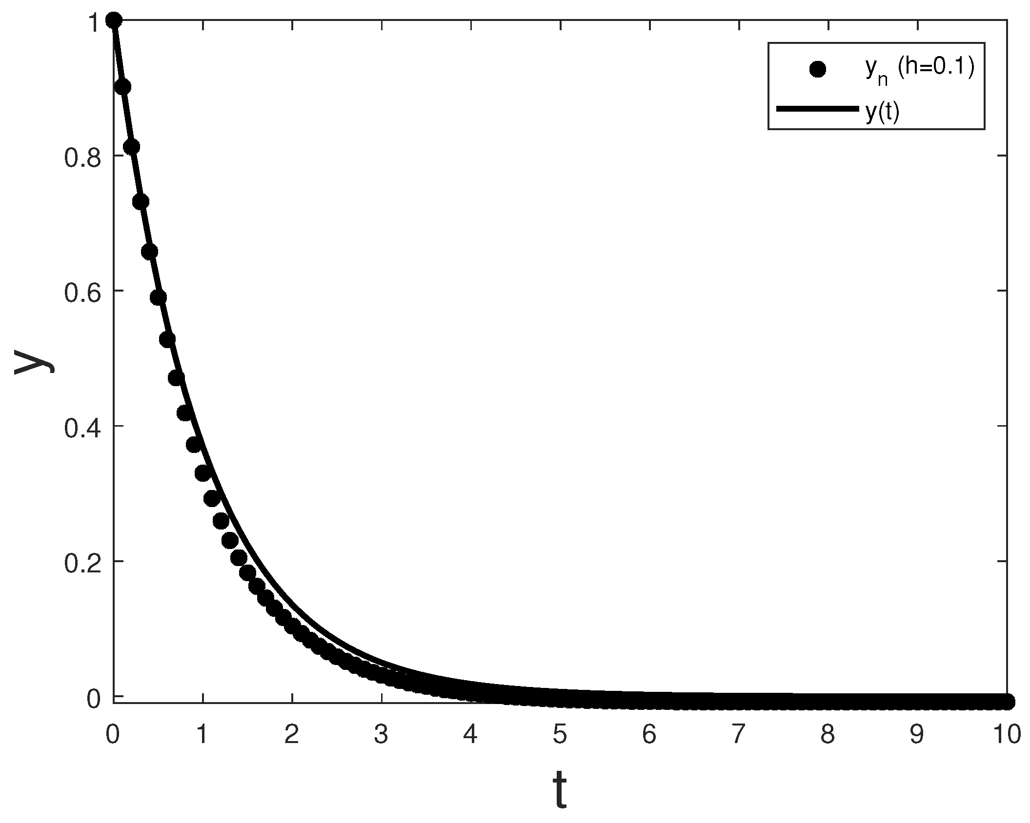
In our first example, we refer to Equation (5) with the kernel k given by

$$k(t,s)=10s{e}^{-s(t+1)},$$

(27)

and the forcing term $f\left(t\right)$ such that the solution $y\left(t\right)=e^{-t}.$ Since $f\left(t\right)$ tends to zero as t goes to infinity, all the assumptions of Theorem 3 are satisfied (for example, with $\overline{t}>3.5$), and thus, both the numerical solution and the continuous one vanish. This is also clear in Figure 1.

Figure 1. Numerical solution to problem (27) compared to the analytical one.

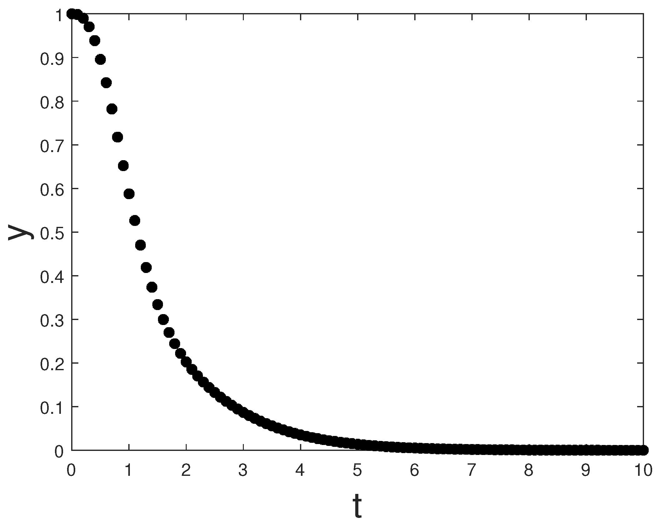
Now, consider Equation (16) with

$$k(t-s)=(t-s)e^{-2(t-s)},G(t,y)=2y\frac{e^{-y^{2}t}}{(1+t^2)(1+y^2)},\mathrm{and} f\left(t\right)=e^{-t^2}.$$

(28)

In Figure 2, we draw the numerical solution obtained with step size $h=0.1,$ which clearly vanishes at infinity, according to Theorem 4, since all assumptions are accomplished with $p\left(t\right)=\frac{2}{1+t^2}$ and $\overline{t}>\frac{1}{2}.$

Figure 2. Numerical solution to problem (28) with $h=0.1.$

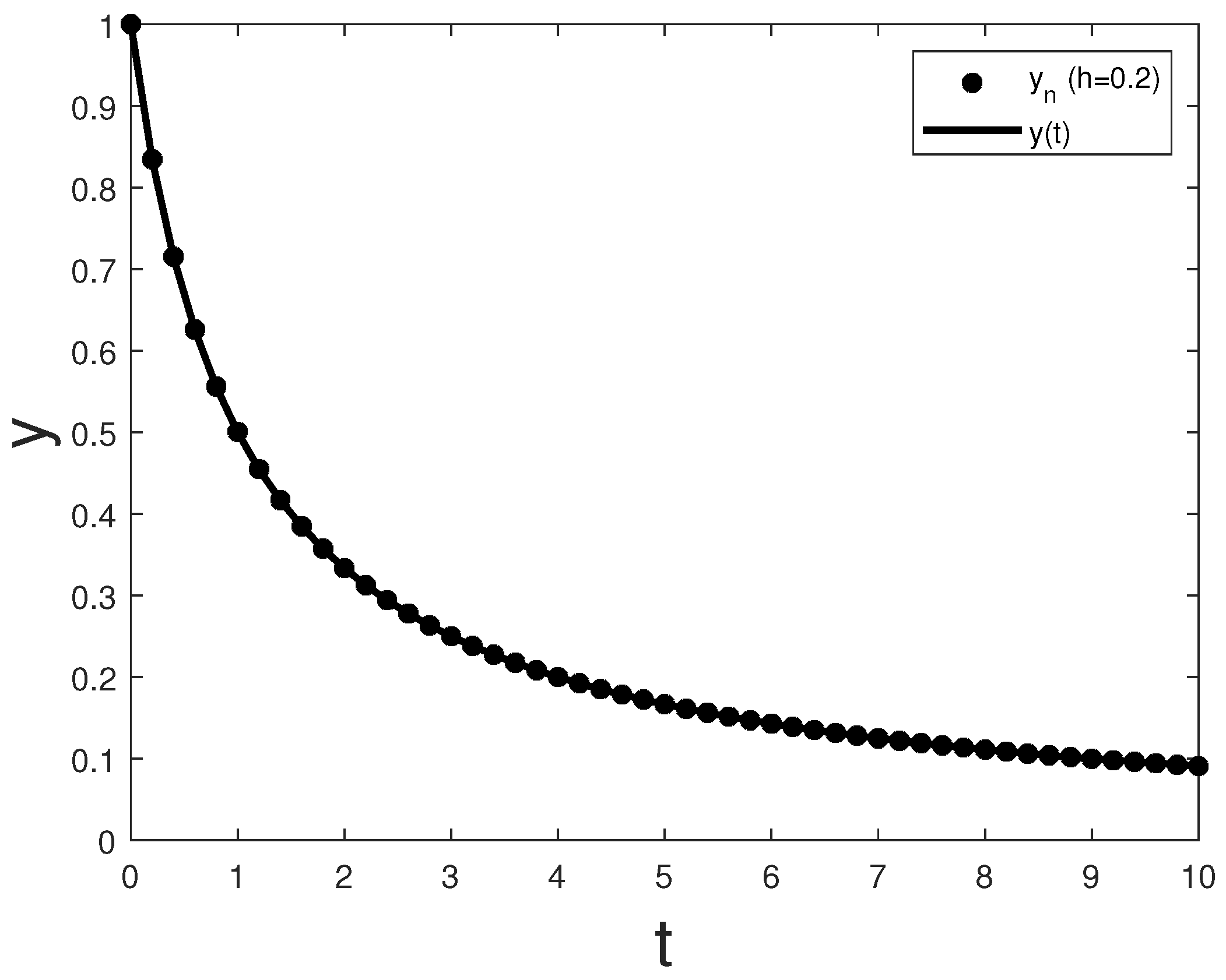
Our third example consists in Equation (5) with

$$k(t,s)=\frac{1}{{(1+2t-s)}^2},$$

(29)

and $f\left(t\right)$ such that the solution $y\left(t\right)=\frac{1}{t+1}.$ According to Theorem 5, with $\phi \left(t\right)={(1+t)}^{-2},$ since $f\left(t\right)$ tends to zero, the numerical solution vanishes regardless of the step size $h,$ thus replicating the asymptotic behaviour of the continuous one. This behaviour is shown in Figure 3.

Figure 3. Numerical solution to problem (29) with h = 0.2, compared to the analytical one.

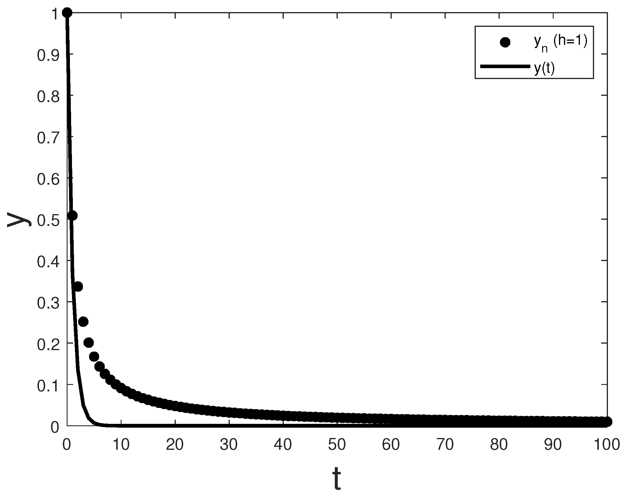
In all our experiments, we used sizes for the meshes that ensure reasonable accuracy in the numerical solution at finite times. Integration with larger discretisation steps naturally introduces greater errors on finite time intervals, but the numerical solution maintains the expected behaviour at infinity. Thus, this confirms the asymptotic-preserving characteristics of the numerical schemes without restrictions on $h.$ This can be observed, for example, in Figure 4, again referring to example (29) with $h=1.$

Figure 4. Numerical solution to problem (29) with h = 1, compared to the analytical one.

6. Conclusions

Starting from an idea developed in [3], here, we have introduced a technique for the analysis of the vanishing behaviour of the numerical solution to VIEs. This new approach, which is based on suitable splittings of the kernel function, allows one to preserve the character of the analytical solution even in the weighted sums that appear in the method, thus leading to unconditional stability results in many applications of interest.