Application of a Maximum Entropy Model for Mineral Prospectivity Maps


1
Geomathematics Key Laboratory of Sichuan Province, Chengdu University of Technology, Chengdu 610059, China
2
Student Affairs Department, China West Normal University, Nanchong 637002, China
3
Institute of Ecological Research, China West Normal University, Nanchong 637002, China
*
Author to whom correspondence should be addressed.
Minerals 2019, 9(9), 556; https://doi.org/10.3390/min9090556
Submission received: 24 July 2019
/
Revised: 10 September 2019
/
Accepted: 12 September 2019
/
Published: 15 September 2019
(This article belongs to the Special Issue Geological Modelling, Volume II)
Abstract
:The effective integration of geochemical data with multisource geoscience data is a necessary condition for mapping mineral prospects. In the present study, based on the maximum entropy principle, a maximum entropy model (MaxEnt model) was established to predict the potential distribution of copper deposits by integrating 43 ore-controlling factors from geological, geochemical and geophysical data. The MaxEnt model was used to screen the ore-controlling factors, and eight ore-controlling factors (i.e., stratigraphic combination entropy, structural iso-density, Cu, Hg, Li, La, U, Na2O) were selected to establish the MaxEnt model to determine the highest potential zone of copper deposits. The spatial correlation between each ore-controlling factor and the occurrence of a copper mine was studied using a response curve, and the relative importance of each ore-controlling factor was determined by jackknife analysis in the MaxEnt model. The results show that the occurrence of copper ore is positively correlated with the content of Cu, Hg, La, structural iso-density and stratigraphic combination entropy, and negatively correlated with the content of Na2O, Li and U. The model’s performance was evaluated by the area under the receiver operating characteristic curve (AUC), Cohen’s maximized Kappa and true skill statistic (TSS) (training AUC = 0.84, test AUC = 0.8, maximum Kappa = 0.5 and maximum TSS = 0.6). The results indicate that the model can effectively integrate multi-source geospatial data to map mineral prospectivity.
1. Introduction
The origins of mineral prospectivity modeling (MPM) can be traced back to mathematical geology, which is an important field of mineral resource evaluation [1,2,3]. Geographic information systems (GIS) establish a spatial prediction model for mineral prospect modeling through comprehensive data sets, such as geological maps, stream sediment geochemical data, aeromagnetic data, etc.
In recent years, with the rapid development of computer technology, many GIS-based mineral prospective analyses and prediction models have been developed. These models can be divided into knowledge-driven, data-driven and hybrid-driven methods. The knowledge-driven methods are based on expert knowledge and the experience of the spatial connection between mineral exploration criteria and the type of deposit sought and is often used in cases where there are insufficient known deposits in the study area, including fuzzy logic [4,5], boolean logic [3,4,5,6], evidential belief modeling [7,8,9], wildcat mapping [10,11], spatial factor analysis [12], etc. Data-driven methods are based on the spatial correlation between known mine sites and multiple exploration datasets and are typically applied to research areas with known deposits/points, such as weights of evidence methods [5,13,14,15,16,17], logistic regression [2,18,19,20], neural networks [21,22,23,24,25], multifractal methods [26,27,28], support vector machines [29,30,31], random forests [32,33,34], etc. The hybrid-driven models combine the advantages of the above two kinds of models, such as fuzzy evidence weight [17,35], fuzzy neural networks [36,37], etc.
The purpose of mineral exploration is to study the relationship between known deposits and ore-controlling factors and then to find new deposits in the area of interest. The idea of this method is similar to the maximum entropy (MaxEnt) model. The MaxEnt model is a statistical model with good performance, which is often used for probabilistic estimation. It is suitable for solving classification problems and is superior to other methods in dealing with many problems, especially when sample data is limited [38,39]. The basic idea of the MaxEnt model is to make the most objective and uniform estimation of unknown events based on satisfying all known events. In recent years, the MaxEnt model has been widely used in natural language processing [40,41], economic prediction [42], geographical distribution of animal and plant species [43] and other fields. Nevertheless, few reports showed that the MaxEnt model was applied in mineral exploration. A MaxEnt model was applied to predict the potential distribution of orogenic gold deposits [44]. However, the parameters negatively related to the mineralization process were not considered and the optimization selection of the β value or regularization multiplier in the model was not discussed in detail.
In the present study, we considered the parameters that negatively correlated with the mineralization process and optimized the regularization multiplier, used geology, geochemistry and geophysical data to establish a MaxEnt model for mineral prospect analysis, and carried out quantitative prediction and evaluation of copper mineralization in the Mila Mountain integrated exploration area to delineate prospecting. The prospective area provides reference and assistance for further prospecting exploration.
2. Study Area and Data
2.1. Study Area
The study area is located in the city of Lhasa, Tibet, China. It is located centrally and south of the Gangdese-Nyainqentanglha (terrain) plate in the Tethys structural area of Tibet (29°10′ N~29°55′ N; 90°45′ E~93°00′ E), with an area of approximately 12,290 km2, and is an important copper metallogenic area in China [45,46,47,48]. The magmatic intrusion in the study area is intense, and the overall spatial distribution is east-west. According to the age of the rock formation, the study area can be divided into Pan-African, Indo-Chinese, Yanshan and Himalayan [49,50]. There are faults in the eras, among them the Mesozoic and Cenozoic intrusive rocks are most closely related to mineralization. The intrusive rocks in the study area are dominated by intermediate-acid intrusive rocks, mostly in the Himalayan period. In space, the intrusive rocks are distributed in various tectonic units, but the different diagenetic environment of each tectonic unit results in different characteristics of the intrusive rocks. The magmatic rocks are well developed in the region, and their spatial distribution is controlled by geotectonic unit belts. There are both exposed areas of deep intrusive bodies and the thick volcano-sedimentary rocks. The magmatic rocks are mainly distributed in the north of the Yajiang fault and are some of the important components of the Gangdese volcano-magma arc [51]. The general trend of the tectonic line in the study area is in an east-west direction. Due to the long-term strike-slip effect of the region, the secondary tectonic lines are mostly in the northwest-west direction, and there could be concealed structures in the north-east direction in the deep part. Due to the impact of the Indian-Eurasian plate collision, several NW-trending nappe structures were developed [52,53]. The main nappe surface is reversed from the deep basin-controlling fault in the passive continental margin period and is now realized as an overthrust fault with ductile-brittle deformation characteristics [53]. The fault structure controls the migration of hydrothermal fluids and controls the intrusion of magmatic rocks, which plays a vital role in mineralization. At present, porphyry copper (molybdenum) deposits, skarn-porphyry copper deposits and skarn copper deposits have been discovered in the study area [54,55]. Most of the known ore deposits are located near the faults, where the ore body (mineralization) is observably controlled by the structure (Figure 1).
2.2. Data
2.2.1. Stratigraphic Combination Entropy
The strata of the study area can be divided into the Gangdese-Tengchong stratigraphic region, the Yarlung Zangbo stratigraphic region and the Himalayan stratigraphic region, and can be further divided into the Lhasa stratigraphic subregion, the Shigatse stratigraphic subregion, the Zhongba stratigraphic subregion, the Zedang stratigraphic subregion and the Kangma-Longzi stratigraphic subregion. The study area contains 43 copper deposits. Through GIS spatial analysis, there are 32 deposits related to stratigraphic space. The strata with the highest proportion of ore deposits is the Yeba formation, followed by the Nyingchi group and the Bima formation (Figure 2). The genesis of the deposits in the study area is magma-pneumatolyto-hydrothermal, and the genetic subtypes of the deposits can be divided into porphyry (vein-disseminated) deposits, vein-altered rock deposits and skarn (contact metasomatism) deposits.
The stratigraphic combination entropy represents the variability of geological bodies per unit area. The more types of geological bodies, the higher the entropy value, the more intense the tectonic activity, the more geomorphologically eroded parts and the more the geological bodies are exposed [56]. Therefore, the stratigraphic combination entropy can reflect the intensity of tectonic activity. It is calculated by the following formula:
where represents the entropy value of the rth geological formation of grid unit and N represents the total number of geological body types (i.e., strata, magmatic rocks, metamorphic rocks and volcanic rocks) in the study area. represents the ratio of the exposed area of the ith stratum to the total grid area.
The definition of stratigraphic combination entropy indicates that the entropy value is positively correlated with the number of stratums per unit area. From a geological point of view, the more intense the tectonic activity, the more geomorphologically eroded parts and the more the stratums are exposed. Therefore, where the stratigraphic entropy is high, the tectonic activity is intense. From the stratigraphic combination entropy map (Figure 3), it can be found that the combined entropy value distribution is correlated with the spatial distribution of fault structures. Ore deposits/mineralization points are mostly located on both sides of the structure, and the location is the gradient of the entropy value transiting from high to low.
2.2.2. Structural Iso-Density
One or more favorable structures are an indispensable factor for magma-hydrothermal mineralization. There are many quantitative indicators for favorable structural information, such as structural iso-density, fracture benefit, structural average orientation, tectonic intersection and structural center symmetry [57,58,59]. These indicators can reflect the characteristics of linear structures from different angles, but they highly correlate with each other. Through the practical study of the mining area, it is found that the structural iso-density can quantitatively describe the developmental part of the favorable structure [59]. It is calculated by the following formula:
where l is the structural iso-density, is the length of the ith linear structure in the prediction unit and is the number of the linear structures. The structural iso-density of the study area (Figure 4) can reflect the complexity of linear structures.
The tertiary geotectonic unit in the study area belongs to the Ladakh-South Gangdise-Lizhao magma arc belt. This area is affected by the northward subduction of the Yarlung Zangbo River arc, the Indian-Asian collision and the post-collision extension. The fault structure in this area is extremely well developed. The structure of the study area is characterized by the development of EW to the main fault, and the development of NE and NW to the compression-torsional secondary fault. It is reflected in the structural iso-density map (Figure 4). The high-density areas are widely distributed in the study area.
It can be seen from the spatial superposition analysis of the known ore deposits/mineralization points that most of the known ore deposits/mineralization points are distributed in the low value areas of structural iso-density, which is a consequence of ore bodies being placed on the side of the fracture. Therefore, structural iso-density value region can be used as an ore-controlling factor for quantitative mineral prediction.
2.2.3. Structural Buffer
Because ore bodies are located to the side of the fault structure, the construction buffer can be used as another means of quantitative information extraction [59]. According to GIS spatial buffer analysis (Figure 5), there are 11 ore deposits/mineralization points in the study area. These deposits are concentrated within a 2 km buffer zone of faults, accounting for 25.6% of the known ore deposits/mineralization points, and 27 ore deposits/mineralization points in the study area are concentrated within a 4 km buffer zone of faults, accounting for 62.8% of the known ore deposits/mineralization points. Besides, we find that the number of deposits/mineralization points do not significantly increase with the enlargement of buffer zone. Therefore, constructing a 4 km buffer can be used as an ore-controlling factor for mineralization prediction.
2.2.4. Aeromagnetic Data
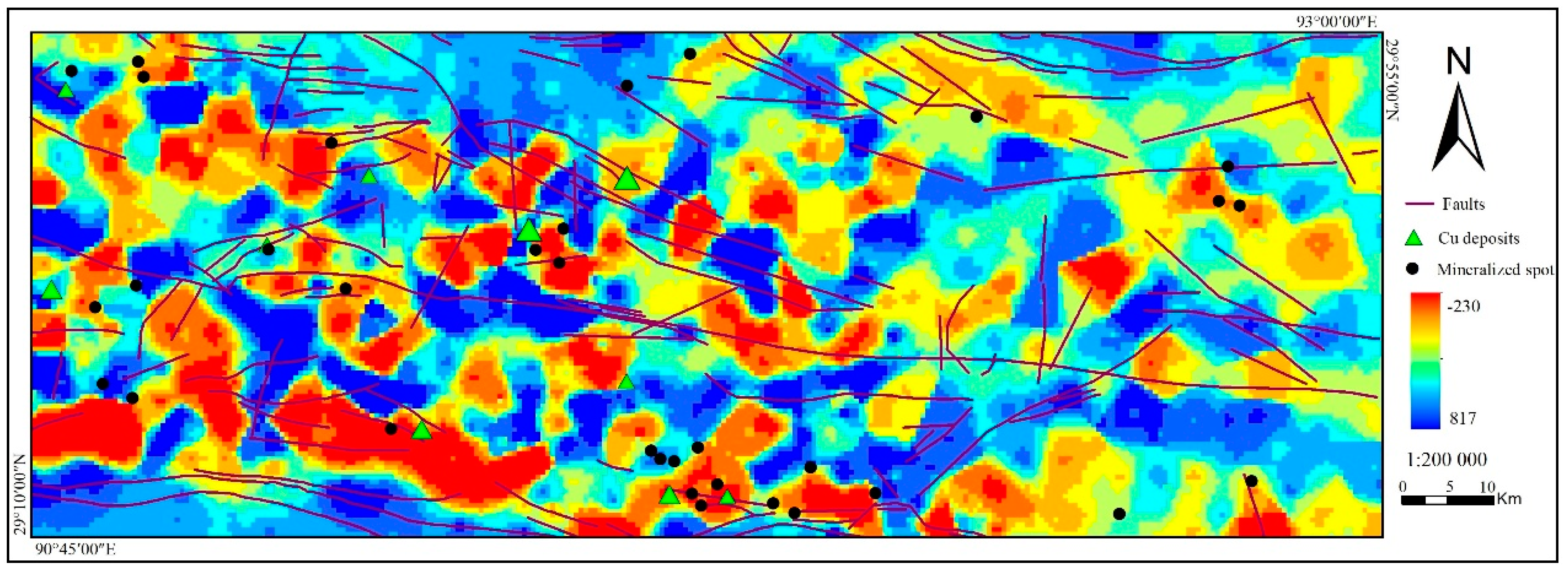
The porphyry copper deposits in the study area have obvious aeromagnetic anomalies and can be used as direct detectors for copper mineralization [60]. The vertical first-order derivative map of the regional aeromagnetic ∆T produced from the reduction to the pole image indicates good correspondence with the rock mass. Overall, Figure 6 shows large changes, where there is a change in the geological units. The known mineral deposits/mineralization points are mostly distributed in the aeromagnetic ∆T by reduction to the pole based on the vertical first-order derivative positive and the negative anomaly transition zone or the positive anomaly parts of the transition zone (Figure 6). Therefore, aeromagnetic data can be used as an ore-controlling factor for mineralization prediction.
2.2.5. Geochemical Data
In the present study, the geochemical data were from 4141 stream sediment samples collected in the study area (Figure 7). The samples were distributed in equal intervals of 2 km × 2 km in space, but the samples were missing in some areas due to terrain conditions and other restrictions. A total of 39 elements were analyzed (i.e., Bi, Cu, P, La, Li, Ag, Sn, Au, Mo, Th, U, W, Sb, Hg, Mn, Cr, Sr, Nb, Pb, Ni, Ti, Y, Cd, Co, Ba, Be, V, Zn, B, As, Zr, F, Fe2O3, K2O, CaO, MgO, Na2O, Al2O3, SiO2) by various methods (mainly inductively coupled plasma-mass spectrometry (ICP-MS), X-ray fluorescence (XRF), inductively coupled plasma-atomic emission spectroscopy (ICP-AES), etc.), and the specific test methods, detection limits, quality control and other information corresponding to each element can be found in relevant literature [61,62].
Traditional methods of exploration using geochemical data usually only consider the identification of positive geochemical anomalies associated with mineralization, while ignoring negative geochemical anomalies [63,64,65,66]. However, the formation of magmatic-hydrothermal mineralization is a complex process, and positive geochemical anomalies alone cannot fully reflect the mineralized geochemical characteristics, resulting in uncertainty of geochemical prospecting [67,68]. Therefore, these 39 elements were taken as ore-controlling factors for mineralization prediction in the present study. The spatial distribution of these 39 elements was obtained by using distance inverse weighted interpolation in ArcGIS 10.2 (Esri, CA, USA) with a grid size of 2 km × 2 km.
3. Construction of the Maximum Entropy Model
The concept of information entropy was first introduced by Shannon in 1948 [69]. It is the expected value of information contained in a message [70]. As a measure of the uncertainty of random events, information entropy can be explicitly written as follows:
where is the information entropy and is the probability of the ith random event.
Jayne [71] proposed a standard that must be subject to precisely stated prior data, and the probability distribution which best represents the current state of knowledge is the one with the largest entropy. This standard is known as the maximum entropy principle.
The MaxEnt model based on the principle of maximum entropy originates from statistical mechanics and is a log-linear model [71]. When predicting the probability distribution of a random event, the prediction should satisfy all known constraints without making any subjective assumptions about the unknown situation. In this case, the probability distribution is the most uniform and the prediction risk is minimum, so the entropy of the probability distribution is maximum [72].
The MaxEnt model, which is a statistical model with good performance, is often used for the probability estimation of problems. It is suitable for solving classification problems and has advantages that other models cannot match [73]. First, the MaxEnt model obtains the model with the maximum information entropy among all the models satisfying the constraint conditions. Second, the MaxEnt model can set the constraint conditions flexibly, moreover, the fitness of the model to unknown data and the degree of fitting to known data can be adjusted by the number of constraints. Third, the MaxEnt model can naturally solve the problem of parameter smoothing in a statistical model. For the exploration of mineral resources, the MaxEnt model mainly obtains the prediction model based on the actual distribution of known mineral deposits and the calculation of various ore-controlling factors in the region, and then obtains the possible distribution of target minerals in the target region. In the present study, MaxEnt software is used to establish the prediction model of the prospective area of mineral resources (MaxEnt 3.3.3k, http://biodiversityinformatics.amnh.org/open_source/maxent/), and the model requires that the ore control factor input must be in the format of an ESRI ASCII (American Standard Code for Information Interchange) grid.
Too many ore-controlling factors or inappropriate parameter settings in the MaxEnt software (e.g., regularization multiplier, maximum iterations, replicated run type, etc.) may lead to a too large, overfit or redundant model. To improve the prediction accuracy of the model and the ability to identify the key ore-controlling factors that limit the mineral distribution, it is necessary to optimize the variables and model parameters in the MaxEnt software. Studies have shown that inappropriate setting of the β value, also known as the regularization multiplier, can lead to overfitting of the model. The smaller the β value, the closer the fitting between the prediction distribution and the training data set will be, while an overfit model cannot reasonably predict the distribution of mineral resources [74]. Relevant studies show that the optimal regularization multiplier is generally higher than the MaxEnt software default value of 1, and the comprehensive performance of the model with a regularization multiplier between 2 and 4 is the best [75]. Therefore, we tried testing different β values (from 2 to 4 with a step size of 0.5) to find the best β value for a particular model. The specific implementation steps are as follows:
- (1)
- Enter the selected β value in the MaxEnt software and set the remaining parameters (a maximum of 500 iterations, a maximum convergence threshold of 0.00001, a maximum of 10,000 background points and the replicated run type set to bootstrap) to the default values;
- (2)
- Create a MaxEnt model containing all variables, eliminate the variable with a contribution rate <1%, and eliminate the variable with the Pearson’s correlation coefficient of the highest contribution variable >0.7 to get model 1;
- (3)
- Establish a new MaxEnt model with the remaining variables, eliminate the variables with a contribution rate <1%, and remove the variables with a correlation coefficient of >0.7 with the second highest contribution variable to get model 2;
- (4)
- Repeat the above process until there is no variable with a contribution rate <1%, and get model M;
- (5)
- Change the β value in the MaxEnt software, and set the remaining parameters to the default values; repeat steps 2–4 to obtain a series of MaxEnt models for the distribution of mineral resources;
- (6)
The lower the AICc value, the higher the model complexity and the more representative the model [78,79]. Therefore, the final MaxEnt model is constructed using the variables in the model with the lowest AICc value. The mineral deposits and data were randomly selected from the dataset during the simulation, with 75% as training data and the remaining 25% for validating the model. To reduce the randomness of the simulation results, the final model was simulated 20 times. Each simulation used the built-in function (contribution of variables, response curve and jackknife analysis) to analyze the relative importance of each variable in modeling and their relationship with favorable metallogenic locations. We used the average output of 20 repeated simulations as the final prediction result. The output is a continuous raster map of the probability of copper metallogenesis in the integrated exploration area of Mila mountain, whose value is between 0 and 1.
The area under the receiver operating characteristic curve (AUC), Cohen’s maximized Kappa and true skill statistics (TSS) were used to evaluate the performance of the established MaxEnt model. These three indicators were calculated based on the specificity and sensitivity of the prediction model. Sensitivity, also known as the true positive rate, refers to the percentage of positive samples that are correctly identified by the classifier as mineralized. Specificity, the true negative rate, represents the percentage of negative samples that are correctly identified by the classifier as not mineralized. AUC is a threshold-independent evaluation measure obtained by plotting sensitivity against 1-specificity [80]. A model accuracy AUC value greater than 0.9 can be judged to be excellent, 0.8 < AUC < 0.9 is good, 0.7 < AUC < 0.8 is general, 0.6 < AUC < 0.7 is poor and 0.5 < AUC < 0.6 is failure [81]. Kappa and TSS are threshold-dependent indexes that measure the agreement between predictions and known occurrences (presences and absences) at different binary thresholds and can also be used to measure classification accuracy. Kappa index can be obtained by plotting sensitivity and specificity against different thresholds [82], while TSS = sensitivity + specificity − 1 [83]. The evaluation criteria for model performance are as follows: Kappa > 0.75 is excellent, 0.4 < Kappa < 0.75 is good and Kappa < 0.4 is poor [84]; TSS > 0.8 is excellent, 0.5 < TSS < 0.8 is available and TSS < 0.5 is poor [85].
In the present study, we used the maximum values of Kappa and TSS under their respective optimal thresholds to evaluate the model performance. Since these two indexes require the use of absence data, 43 points were randomly selected as pseudo-absence points within the study area (43 known ore deposits/mineralization points). These pseudo-absence points were randomly located outside the 4 km buffer of the known ore deposits/mineralization points. Threshold-dependent statistics were analyzed in R3.2.2 [86] with package “Presence Absence” [87].
For further analysis, we used the maximum value of TSS to obtain an optimal threshold and convert the continuous raster map of mineralization prediction probability into a binary favorable metallogenic/background map. When only known ore/mineralization points were available, the maximum value of TSS could be used as an evaluation criterion for determining whether the threshold is optimal, and it is superior to many other standards in most cases [88]. Based on the determined optimal threshold, we estimated the total area of copper metal ore predictions in the Mila Mountain integrated exploration area.
4. Results
4.1. Model Performance Evaluation
According to the above algorithm flow, the MaxEnt model was established using 43 ore-controlling factors in the Mila Mountain integrated exploration area (Appendix A), and the AICc value of each model was calculated. The calculation results are shown in Table 1. It can be seen from Table 1 that model 6 has the minimum AICc value, so this model was selected to be the optimal model, β = 2.5, and the model factors are: stratigraphic combination entropy, structural iso-density, Cu, Hg, Li, La, U, Na2O (The distributions of elements Cu, Hg, Li, La, U and Na2O are shown in Figure 8). The MaxEnt software was used to perform 20 replicated simulations on the optimal model. To construct the model during the simulation, 75% of data were randomly selected from data sets (43 known deposits/points). The remaining 25% of data were used to validate the test data. Table 2 lists the training AUC and test AUC of the total 20 simulations. Table 2 shows that the average training AUC = 0.84 and the average test AUC = 0.8. The Kappa and TSS values were calculated using the R3.2.2 with package “Presence Absence”, the maximum Kappa = 0.5 and the maximum TSS = 0.6. All evaluation indexes of the model indicated that the model has a good ability to identify favorable/unfavorable areas for copper mineralization. Therefore, we think that the model is reliable and acceptable.
4.2. Predictive Variable Contribution
Table 3 shows the contribution rate of each ore-controlling factor to the model. The contribution of variables represents the percent contribution of variables to the model. Among them, copper is the most important ore-controlling factor for indicating the occurrence of copper deposits. It reflects the contribution to the deposits from the perspective of the change of elemental content. Copper accounts for 38.1% of the total contribution. Na2O and Li are the second and third most important ore-controlling factors, respectively. Na and Li are typical lithophile elements, which can reflect the relationship between intermediate-acid rocks, basic-ultrabasic rocks and copper mineralization. Hg is a typical chalcophile element, which has an important impact on predicting the occurrence of copper deposits. Table 3 shows that four predictors (i.e., Cu, Na2O, Li and Hg) had over 10% of relative contribution to the copper-metal ore prediction model in the Mila Mountain integrated exploration area, contributing 74% collectively. The importance of each ore-controlling factor on the prediction rate of copper prospects was examined through the jackknife analysis (Figure 9). Jackknife analysis evaluates the influence of each predictor variable on the MaxEnt model. The method sequentially precludes one ore-controlling factor from the analysis and runs the MaxEnt model using the rest of the variables, and again, runs the model separately using the precluded variable only. Therefore, the share of each ore-controlling factor on the total gain of the model can be calculated. The importance of the first four main ore-controlling factors is basically consistent with the contribution rate of modeling.
4.3. Response Curves of the Ore-Controlling Factors
Response curves show how each ore-controlling factor affects the logistic prediction when all variables are used to build a full model. The response curves reflect the spatial relationship between the ore-controlling factor and the favorable degree of copper deposits. The larger the value on the y-axis of the response curve, the greater the logistic probability of forming a copper deposit (Figure 10). The curves show the mean response of 20 replicate MaxEnt runs (red) and the mean +/− one standard deviation (blue, two shades for categorical variables). Figure 10 shows that the favorable degree of copper ore occurrence is positively correlated with the content of Cu, Hg, La, structural iso-density and stratigraphic combination entropy, and negatively correlated with the content of Na2O, Li and U.
4.4. Perspective Map of Copper
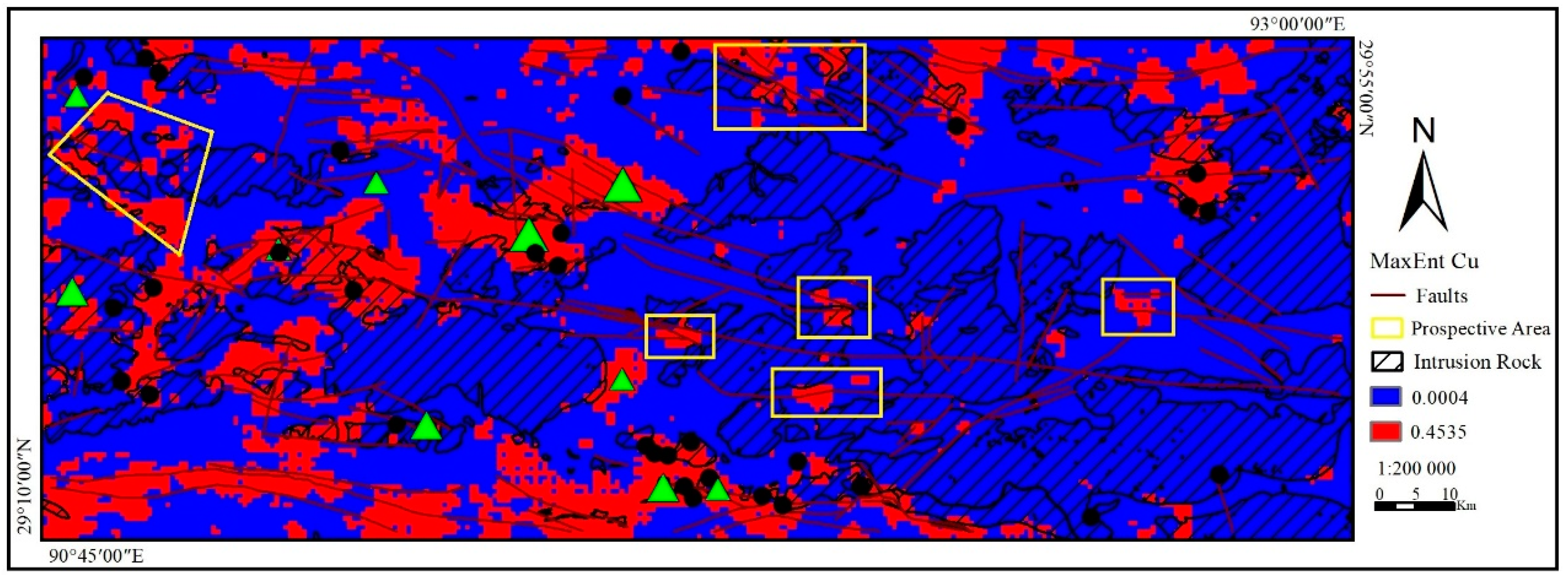
The output of the MaxEnt model was mapped to a continuous scale perspective in ArcGIS10.2 (Figure 11), and the logistic probability ranged from 0.0004 to 0.9247. Although the continuous-scale perspective shows a good relationship between the high probability and known copper ore locations, it is difficult to explain the exploration target in terms of continuous variable logistic probability. Therefore, the TSS maximum value is used to obtain an optimal threshold (optimal threshold = 0.4535), which converts the continuous grid diagram of metallogenic prediction probability into a binary map of favorable metallogenic area/background area (Figure 12). Red represents the favorable metallogenic area, accounting for 21.1% of the total study area, containing 72.2% of the total number of copper deposits/mineralization points.
5. Discussion
In recent years, many techniques have been developed to study the spatial relationship between ore-controlling factors and known ore deposits/mineralization points, such as the weight of evidence method [18] and the random forest method [33]. Here, the response curve analysis in the MaxEnt software can be regarded as a very useful tool, through which the change of logistic probability between various variables and the target deposits can be intuitively observed [38]. Based on the maximum entropy principle, the present study integrates 43 ore-controlling factors from geological, geochemical and geophysical data which relate to the mineralization process and construct the MaxEnt model for mineral prospect prediction. Through the contribution rate and Pearson’s correlation coefficient of each ore-controlling factor, the ore-controlling factors were screened, different MaxEnt models were established by using different β-values and the superiority of the model was evaluated by AICc criteria. Finally, the MaxEnt model was constructed by stratigraphic combination entropy, structural iso-density, Cu, Hg, Li, La, U, Na2O. The control coefficient β of the model = 2.5, and the remaining parameters were set to the default values. Figure 10 shows that the favorable degree of copper ore occurrence is positively correlated with the content of Cu, Hg, La, structural iso-density and stratigraphic combination entropy, and negatively correlated with the content of Na2O, Li and U.
The importance of ore-controlling factors can be ranked by jackknife analysis, sometimes this sorting may not reflect actual knowledge of ore-controlling conditions. For example, stratigraphic combination entropy and structural iso-density are important indicators for discovering metallogenic areas [56,59], however, our research shows that their contribution to the MaxEnt model is relatively small (Table 3). By observing ore-controlling factors after screening, we also obtain some interesting findings. Hg is a typical chalcophile element [89]. It has high content in alkaline rock and has a good indicating effect for copper exploration. As a rare earth element, La has rarely been noticed in previous mineral explorations. Previous studies have shown that rare earth elements are weakly alkaline and have high content in alkaline rocks and granites, especially in calcium-bearing rock-forming minerals [90]. The rare earth elements released during the weathering of rocks and deposits mostly migrate in the form of carbonates and organic complexes. Under epigenetic conditions, their ability to migrate in a dissolved state is limited, and the copper deposits in the Mila Mountains are mainly enriched in the calc-alkaline series of rocks. Thus, the La element can be used as an indicator for copper exploration in this area. Negative geochemical anomalies have attracted more and more attention [91,92]. They can provide key information about basic geological and geochemical anomaly interpretation and model establishment [93]. Figure 10 shows that the contents of Na2O and Li are negatively correlated with a favorable degree of copper deposits, indicating that the porphyry copper-molybdenum ore is mostly distributed in the negative anomaly of Na2O and other elements formed by the take out effect [94], and as copper mineralization increases, the depletion of Li gradually increases [89,91]. The content of U is negatively correlated with the favorable degree of copper deposits. It is probably during the multi-stage and multi-period evolution of complex rock masses that SiO2, K2O and Na2O in the rock increase gradually, and ore-forming elements such as U, W and Ta gradually increase [90].
We obtained the metallogenic prospect map of the integrated exploration area in the Mila Mountain through the fusion analysis of screened ore-control factors. Figure 11 shows that there is high consistency between the known copper mine location and the continuous high probability values. According to the binary mineralization prospect map (Figure 12), there are many fault development zones in the metallogenic potential area, these areas are places of hydrothermal activity, which can provide transport channels for ore-forming materials extracted from the formation, sedimentation, enrichment, and mineralization in relatively quiet areas beside the tectonic activity. Most of the favorable metallogenic areas are spatially adjacent to the Himalayan intrusive rocks. This is consistent with the geological understanding that magmatism is closely related to mineralization. Therefore, the geochemical anomaly zone can be further refined by examining its relationship with favorable geological features, including whether it is Himalayan intrusive rock or a known ore deposit, and whether it is close to faults. Combined with geological mineralization laws, several predicted prospects were identified, as shown in Figure 13. It is worth noting that large areas of high probability occur in the southwest of the survey area, but those areas are not considered as prediction prospects. This is mainly because those areas are mainly ultrabasic rocks. Previous studies have shown that the content of copper in ultrabasic rocks is generally high, but the contribution of ultrabasic rocks is very small as a source of copper ore deposits [95]. However, these predicted prospects need to be further investigated through field surveys or through geophysical, remote sensing or using other information.
Although the MaxEnt model is convenient and easy to use, the role of model optimization cannot be ignored when using it [78]. If the model is not optimized, the prediction results of the model may have serious overfitting errors, which will not only lead to incorrect evaluation of the metallogenic prospect map, but also result in misleading planning of the metallogenic prospect area. Although the MaxEnt software provides some options for model optimization, there is no clear standard for setting relevant parameters [96]. Therefore, when constructing the MaxEnt model, the selection of relevant parameters needs to be conducted very carefully.
6. Conclusions
(1) The MaxEnt model used in the present study is simple and easy to perform, with high prediction accuracy. It can be used to predict potential distribution and mineralization favorableness of mineralization in the Mila Mountain integrated exploration area.
(2) The MaxEnt model can be used to generate the spatial response curve of each ore-controlling factor to the copper deposit/mineralization point, and the relative importance of each ore-controlling factor to the established model can be tested by jackknife analysis. The AUC, Kappa and TSS values of the present study indicate that the model can correctly classify copper deposits.
(3) The favorable zones shown in the metallogenic prospect map are spatially consistent with known copper deposits/occurrence areas and major mineralization trends. This outcome indicates that the MaxEnt model can be effectively used for spatial fusion analysis of multi-source geospatial data. According to the prospect map and expert knowledge, some areas of interest have been preliminarily delineated to provide references for subsequent exploration research.
Author Contributions
B.L. (Binbin Li) and C.L. processed geochemical data. B.L. (Bingli Liu), K.G. and B.W. provided the idea of processing data. B.L. (Binbin Li) wrote this paper.
Funding
This research was funded by the National Key R&D Program of China (2017YFC0601505), Chinese National Natural Science Foundation (41602334, 41672325), the Key R&D of Science and Technology Department of Sichuan Province (2018SZ0328), and Opening Fund of Geomathematics Key Laboratory of Sichuan Province (scsxdz2018zd03, scsxdz2019zd01).
Conflicts of Interest
The authors have no conflict of interest to declare.
Appendix A

Table A1.
Optimization of the selection process of ore-controlling factors and β values.
| Factors | β = 2 | β = 2.5 | β = 3 | β = 3.5 | β = 4 | |||||||||||||||||||||||||
|---|---|---|---|---|---|---|---|---|---|---|---|---|---|---|---|---|---|---|---|---|---|---|---|---|---|---|---|---|---|---|
| con | cor | con | cor | con | cor | con | cor | con | cor | con | cor | con | cor | con | cor | con | cor | con | cor | con | cor | con | cor | con | cor | con | cor | con | cor | |
| Model | 1 | 1 | 2 | 2 | 3 | 3 | 4 | 4 | 5 | 5 | 6 | 6 | 7 | 7 | 8 | 8 | 9 | 9 | 10 | 10 | 11 | 11 | 12 | 12 | 13 | 13 | 14 | 14 | 15 | 15 |
| Cu | 45.80 | 1.00 | 46.20 | 0.04 | 51.80 | 0.01 | 47.60 | 1.00 | 54.00 | 0.04 | 51.50 | 0.01 | 45.50 | 1.00 | 48.00 | 0.04 | 42.20 | 1.00 | 42.80 | 0.04 | 41.20 | 0.11 | 44.10 | 1.00 | 43.80 | 0.04 | 44.90 | 0.11 | 44.10 | 0.11 |
| Na2O | 16.20 | 0.04 | 17.80 | 1.00 | 18.20 | −0.01 | 16.40 | 0.04 | 16.40 | 1.00 | 18.80 | 0.32 | 20.70 | 0.04 | 20.50 | 1.00 | 26.20 | 0.04 | 27.60 | 1.00 | 27.30 | 0.40 | 28.60 | 0.04 | 29.00 | 1.00 | 30.00 | 0.40 | 29.70 | 0.10 |
| Li | 3.70 | 0.11 | 4.80 | 0.40 | 4.70 | 0.30 | 6.20 | 0.11 | 7.60 | 0.40 | 9.30 | 0.30 | 10.60 | 0.11 | 11.90 | 0.40 | 7.00 | 0.11 | 8.70 | 0.40 | 12.80 | 1.00 | 7.40 | 0.11 | 10.40 | 0.40 | 10.40 | 1.00 | 10.10 | 0.15 |
| W | 1.10 | 0.11 | 0.40 | - | - | - | 0.90 | - | - | - | - | - | 3.30 | 0.11 | 3.70 | 0.10 | 3.50 | 0.11 | 4.90 | 0.10 | 4.30 | 0.15 | 5.60 | 0.11 | 5.60 | 0.10 | 5.80 | 0.15 | 5.70 | 1.00 |
| Structural Iso-density | 1.60 | 0.02 | 3.80 | −0.01 | 2.80 | −0.06 | 3.50 | 0.02 | 3.50 | −0.05 | 2.90 | −0.07 | 2.50 | 0.02 | 2.60 | −0.05 | 4.20 | 0.02 | 4.30 | −0.05 | 4.10 | 0.15 | 4.10 | 0.02 | 4.20 | −0.05 | 4.50 | 0.15 | 4.50 | −0.02 |
| SiO2 | 2.40 | 0.08 | 0.20 | - | - | - | 0.00 | - | - | - | - | - | 0.00 | - | - | - | 3.20 | 0.08 | 1.20 | 0.73 | - | - | 2.50 | 0.08 | 0.00 | - | - | - | - | - |
| U | 10.30 | 0.01 | 10.40 | 0.32 | 8.90 | 1.00 | 10.10 | 0.01 | 9.00 | 0.32 | 8.70 | 1.00 | 7.00 | 0.01 | 5.90 | 0.32 | 5.60 | 0.01 | 5.20 | 0.32 | 5.30 | 0.30 | 2.40 | 0.01 | 2.80 | 0.32 | 1.20 | 0.30 | 1.40 | 0.15 |
| Hg | 3.20 | 0.09 | 3.90 | 0.06 | 3.50 | 0.09 | 4.00 | 0.09 | 5.00 | 0.06 | 4.60 | 0.09 | 3.80 | 0.09 | 3.70 | 0.06 | 3.70 | 0.09 | 2.20 | 0.06 | 2.30 | 0.42 | 1.40 | 0.09 | 2.10 | 0.06 | 2.30 | 0.42 | 4.50 | 0.09 |
| La | 1.70 | 0.14 | 1.50 | 0.50 | 1.80 | 0.37 | 2.00 | 0.14 | 1.80 | 0.50 | 1.90 | 0.37 | 1.70 | 0.14 | 1.50 | 0.50 | 1.50 | 0.14 | 1.30 | 0.50 | 1.20 | 0.62 | 1.00 | 0.14 | 0.90 | - | - | - | - | - |
| Combinatorial Entropy | 1.70 | −0.02 | 2.00 | 0.01 | 2.20 | −0.02 | 2.50 | −0.02 | 2.60 | 0.01 | 2.30 | −0.02 | 2.10 | −0.02 | 2.30 | 0.01 | 1.80 | −0.02 | 1.90 | 0.01 | 1.60 | 0.04 | 1.00 | −0.02 | 1.20 | 0.01 | 0.90 | - | - | - |
| Mo | 1.10 | 0.27 | 1.50 | 0.09 | 3.50 | 0.22 | 0.60 | - | - | - | - | - | 0.20 | - | - | - | 0.00 | - | - | - | - | - | 0.90 | - | - | - | - | - | - | - |
| Cr | 0.00 | - | - | - | - | - | 0.20 | - | - | - | - | - | 0.50 | - | - | - | 0.00 | - | - | - | - | - | 0.70 | - | - | - | - | - | - | - |
| Aeromagnetic Data | 0.90 | - | - | - | - | - | 0.80 | - | - | - | - | - | 0.60 | - | - | - | 0.50 | - | - | - | - | - | 0.30 | - | - | - | - | - | - | - |
| Sb | 1.70 | 0.13 | 0.30 | - | - | - | 0.70 | - | - | - | - | - | 0.10 | - | - | - | 0.00 | - | - | - | - | - | 0.10 | - | - | - | - | - | - | - |
| Ag | 0.10 | - | - | - | - | - | 0.10 | - | - | - | - | - | 0.00 | - | - | - | 0.00 | - | - | - | - | - | 0.00 | - | - | - | - | - | - | - |
| Al2O3 | 0.00 | - | - | - | - | - | 0.00 | - | - | - | - | - | 0.00 | - | - | - | 0.00 | - | - | - | - | - | 0.00 | - | - | - | - | - | - | - |
| As | 0.10 | - | - | - | - | - | 0.10 | - | - | - | - | - | 0.00 | - | - | - | 0.00 | - | - | - | - | - | 0.00 | - | - | - | - | - | - | - |
| Au | 0.00 | - | - | - | - | - | 0.00 | - | - | - | - | - | 0.00 | - | - | - | 0.00 | - | - | - | - | - | 0.00 | - | - | - | - | - | - | - |
| B | 0.00 | - | - | - | - | - | 0.00 | - | - | - | - | - | 0.00 | - | - | - | 0.00 | - | - | - | - | - | 0.00 | - | - | - | - | - | - | - |
| Ba | 0.10 | - | - | - | - | - | 0.00 | - | - | - | - | - | 0.00 | - | - | - | 0.00 | - | - | - | - | - | 0.00 | - | - | - | - | - | - | - |
| Be | 0.00 | - | - | - | - | - | 0.00 | - | - | - | - | - | 0.00 | - | - | - | 0.00 | - | - | - | - | - | 0.00 | - | - | - | - | - | - | - |
| Bi | 0.10 | - | - | - | - | - | 0.00 | - | - | - | - | - | 0.00 | - | - | - | 0.00 | - | - | - | - | - | 0.00 | - | - | - | - | - | - | - |
| CaO | 1.10 | 0.05 | 0.20 | - | - | - | 0.80 | - | - | - | - | - | 0.30 | - | - | - | 0.00 | - | - | - | - | - | 0.00 | - | - | - | - | - | - | - |
| Cd | 0.20 | - | - | - | - | - | 0.00 | - | - | - | - | - | 0.00 | - | - | - | 0.00 | - | - | - | - | - | 0.00 | - | - | - | - | - | - | - |
| Co | 0.00 | - | - | - | - | - | 0.00 | - | - | - | - | - | 0.00 | - | - | - | 0.00 | - | - | - | - | - | 0.00 | - | - | - | - | - | - | - |
| Structural Buffer | 1.00 | 0.05 | 0.70 | - | - | - | 0.20 | - | - | - | - | - | 0.00 | - | - | - | 0.00 | - | - | - | - | - | 0.00 | - | - | - | - | - | - | - |
| F | 0.00 | - | - | - | - | - | 0.00 | - | - | - | - | - | 0.00 | - | - | - | 0.00 | - | - | - | - | - | 0.00 | - | - | - | - | - | - | - |
| Fe2O3 | 0.00 | - | - | - | - | - | 0.00 | - | - | - | - | - | 0.00 | - | - | - | 0.00 | - | - | - | - | - | 0.00 | - | - | - | - | - | - | - |
| K2O | 0.00 | - | - | - | - | - | 0.00 | - | - | - | - | - | 0.00 | - | - | - | 0.00 | - | - | - | - | - | 0.00 | - | - | - | - | - | - | - |
| MgO | 0.00 | - | - | - | - | - | 0.00 | - | - | - | - | - | 0.00 | - | - | - | 0.00 | - | - | - | - | - | 0.00 | - | - | - | - | - | - | - |
| Mn | 0.00 | - | - | - | - | - | 0.00 | - | - | - | - | - | 0.00 | - | - | - | 0.00 | - | - | - | - | - | 0.00 | - | - | - | - | - | - | - |
| Nb | 0.60 | - | - | - | - | - | 0.50 | - | - | - | - | - | 0.30 | - | - | - | 0.00 | - | - | - | - | - | 0.00 | - | - | - | - | - | - | - |
| Ni | 0.80 | - | - | - | - | - | 0.00 | - | - | - | - | - | 0.00 | - | - | - | 0.00 | - | - | - | - | - | 0.00 | - | - | - | - | - | - | - |
| pb | 0.00 | - | - | - | - | - | 0.80 | - | - | - | - | - | 0.50 | - | - | - | 0.20 | - | - | - | - | - | 0.00 | - | - | - | - | - | - | - |
| Pb | 0.00 | - | - | - | - | - | 0.00 | - | - | - | - | - | 0.00 | - | - | - | 0.00 | - | - | - | - | - | 0.00 | - | - | - | - | - | - | - |
| Sn | 0.00 | - | - | - | - | - | 0.00 | - | - | - | - | - | 0.00 | - | - | - | 0.00 | - | - | - | - | - | 0.00 | - | - | - | - | - | - | - |
| Sr | 0.10 | - | - | - | - | - | 0.10 | - | - | - | - | - | 0.00 | - | - | - | 0.00 | - | - | - | - | - | 0.00 | - | - | - | - | - | - | - |
| Th | 0.00 | - | - | - | - | - | 0.00 | - | - | - | - | - | 0.00 | - | - | - | 0.00 | - | - | - | - | - | 0.00 | - | - | - | - | - | - | - |
| Ti | 0.20 | - | - | - | - | - | 0.00 | - | - | - | - | - | 0.00 | - | - | - | 0.00 | - | - | - | - | - | 0.00 | - | - | - | - | - | - | - |
| V | 0.00 | - | - | - | - | - | 0.00 | - | - | - | - | - | 0.00 | - | - | - | 0.00 | - | - | - | - | - | 0.00 | - | - | - | - | - | - | - |
| Y | 0.50 | - | - | - | - | - | 0.60 | - | - | - | - | - | 0.30 | - | - | - | 0.20 | - | - | - | - | - | 0.00 | - | - | - | - | - | - | - |
| Zn | 2.40 | 0.26 | 6.30 | 0.17 | 2.60 | 0.16 | 1.40 | 0.26 | 0.20 | - | - | - | 0.00 | - | - | - | 0.00 | - | - | - | - | - | 0.00 | - | - | - | - | - | - | - |
| Zr | 0.50 | - | - | - | - | - | 0.00 | - | - | - | - | - | 0.00 | - | - | - | 0.00 | - | - | - | - | - | 0.00 | - | - | - | - | - | - | - |
Note: “-” represents the ore-controlling factor not participating in model calculation. The “con” represents the percent contribution, and the “cor” represents the Pearson’s correlation coefficient.
References
- Harris, D.P. An Application of Multivariate Statistical Analysis to Mineral Exploration. Ph.D. Thesis, The Pennsylvania State University, State College, PA, USA, 1965. [Google Scholar]
- Agterberg, F. Automatic contouring of geological maps to detect target areas for mineral exploration. Math. Geol. 1974, 6, 373–395. [Google Scholar] [CrossRef]
- Bonham-Carter, G.F. Geographic Information Systems for Geoscientists: Modelling with GIS; Elsevier: Amsterdam, The Netherlands, 1994; Volume 13, p. 416. [Google Scholar]
- An, P.; Moon, W.; Rencz, A. Application of fuzzy set theory for integration of geological, geophysical and remote sensing data. Can. J. Explor. Geophys. 1991, 27, 1–11. [Google Scholar]
- Ford, A.; Miller, J.M.; Mol, A.G. A comparative analysis of weights of evidence, evidential belief functions, and fuzzy logic for mineral potential mapping using incomplete data at the scale of investigation. Nat. Resour. Res. 2016, 25, 19–33. [Google Scholar] [CrossRef]
- Carranza, E.J.M.; Mangaoang, J.C.; Hale, M. Application of mineral exploration models and GIS to generate mineral potential maps as input for optimum land-use planning in the Philippines. Nat. Resour. Res. 1999, 8, 165–173. [Google Scholar] [CrossRef]
- An, P.; Moon, W.; Bonham-Carter, G. Uncertainty management in integration of exploration data using the belief function. Nonrenew. Res. 1994, 3, 60–71. [Google Scholar] [CrossRef]
- Carranza, E.; Woldai, T.; Chikambwe, E. Application of data-driven evidential belief functions to prospectivity mapping for aquamarine-bearing pegmatites, Lundazi district, Zambia. Nat. Resour. Res. 2005, 14, 47–63. [Google Scholar] [CrossRef]
- Carranza, E.J.M. Geochemical Anomaly and Mineral Prospectivity Mapping in GIS; Elsevier: Amsterdam, The Netherlands, 2008; Volume 11, p. 365. [Google Scholar]
- Carranza, E.J.M. Improved wildcat modelling of mineral prospectivity. Resour. Geol. 2010, 60, 129–149. [Google Scholar] [CrossRef]
- Carranza, E.; Hale, M. Wildcat mapping of gold potential, Baguio district, Philippines. Appl. Earth Sci. 2002, 111, 100–105. [Google Scholar] [CrossRef]
- Grunsky, E.; Agterberg, F. The application of spatial factor analysis to unconditional simulations with implications for mineral exploration. In Proceedings of the 21st International Symposium on Computers in the Mineral Industry; Society of Mining Engineers of AIME: Las Vegas, NV, USA, 1989; pp. 194–208. [Google Scholar]
- Agterberg, F.P. Combining indicator patterns in weights of evidence modeling for resource evaluation. Nonrenew. Res. 1992, 1, 39–50. [Google Scholar] [CrossRef]
- Bonham-Carter, G.F. Weights of evidence modeling: A new approach to mapping mineral potential. Stat. Appl. Earth Sci. 1989, 98, 171–183. [Google Scholar]
- Liu, Y.; Cheng, Q.; Xia, Q.; Wang, X. Mineral potential mapping for tungsten polymetallic deposits in the Nanling metallogenic belt, South China. J. Earth Sci. 2014, 25, 689–700. [Google Scholar] [CrossRef]
- Ziaii, M.; Pouyan, A.; Ziaei, M. A computational optimized extended model for mineral potential mapping based on W of E method. Am. J. Appl. Sci. 2009, 6, 200–203. [Google Scholar]
- Cheng, Q.; Chen, Z.; Khaled, A. Application of fuzzy weights of evidence method in mineral resource assessment for gold in Zhenyuan District, Yunnan Province, China. Earth Sci. 2007, 32, 175–184. [Google Scholar]
- Agterberg, F.; Bonham-Carter, G. Logistic regression and weights of evidence modeling in mineral exploration. In Proceedings of the 28th International Symposium on Applications of Computer in the Mineral Industry (APCOM), Golden, CO, USA, 20–22 October 1999; p. 490. [Google Scholar]
- Carranza, E.; Hale, M.; Faassen, C. Selection of coherent deposit-type locations and their application in data-driven mineral prospectivity mapping. Ore Geol. Rev. 2008, 33, 536–558. [Google Scholar] [CrossRef]
- Chen, C.; Dai, H.; Liu, Y.; He, B. Mineral prospectivity mapping integrating multi-source geology spatial data sets and logistic regression modelling. In Proceedings of the 2011 IEEE International Conference on Spatial Data Mining and Geographical Knowledge Services, Fuzhou, China, 29 June–1 July 2011; pp. 214–217. [Google Scholar]
- Brown, W.M.; Gedeon, T.; Groves, D.; Barnes, R. Artificial neural networks: A new method for mineral prospectivity mapping. Aust. J. Earth Sci. 2000, 47, 757–770. [Google Scholar] [CrossRef]
- Skabar, A. Mineral potential mapping using feed-forward neural networks. In Proceedings of the International Joint Conference on Neural Networks, Portland, OR, USA, 20–24 July 2003; pp. 1814–1819. [Google Scholar]
- Leite, E.P.; de Souza Filho, C.R. Artificial neural networks applied to mineral potential mapping for copper-gold mineralizations in the Carajás Mineral Province, Brazil. Geophys. Prospect. 2009, 57, 1049–1065. [Google Scholar] [CrossRef]
- Leite, E.P.; de Souza Filho, C.R. Probabilistic neural networks applied to mineral potential mapping for platinum group elements in the Serra Leste region, Carajás Mineral Province, Brazil. Comput. Geosci. 2009, 35, 675–687. [Google Scholar] [CrossRef]
- Oh, H.-J.; Lee, S. Application of artificial neural network for gold–silver deposits potential mapping: A case study of Korea. Nat. Resour. Res. 2010, 19, 103–124. [Google Scholar] [CrossRef]
- Cheng, Q.M. Singularity-generalized self-similarity-fractal spectrum (3S) models. Earth Sci. 2006, 31, 337–348. [Google Scholar]
- Cheng, Q.M.; Zhao, P.D.; Chen, J.G.; Xia, Q.L.; Chen, Z.J.; Zhan, S.Y.; Xu, D.Y.; Xia, X.Y.; Wan, W.L. Application of singularity theory in prediction of tin and copper mineral deposits in Gejiu district, Yunnan, China: Weak information extraction and mixing information decomposition. Earth Sci. 2009, 34, 243–252. [Google Scholar]
- Liu, B.; Guo, K.; Li, C.; Zhou, J.; Liu, X.; Wang, X.; Wang, L. Copper prospectivity in Tibet, China: Based on the identification of geochemical anomalies. Ore Geol. Rev. 2018. [Google Scholar] [CrossRef]
- Abedi, M.; Norouzi, G.H.; Bahroudi, A. Support vector machine for multi-classification of mineral prospectivity areas. Comput. Geosci. 2012, 46, 272–283. [Google Scholar] [CrossRef]
- Zuo, R.; Carranza, E.J.M. Support vector machine: A tool for mapping mineral prospectivity. Comput. Geosci. 2011, 37, 1967–1975. [Google Scholar] [CrossRef]
- Geranian, H.; Tabatabaei, S.H.; Asadi, H.H.; Carranza, E.J.M. Application of discriminant analysis and support vector machine in mapping gold potential areas for further drilling in the Sari-Gunay gold deposit, NW Iran. Nat. Resour. Res. 2016, 25, 145–159. [Google Scholar] [CrossRef]
- Rodriguez-Galiano, V.F.; Chica-Olmo, M.; Chica-Rivas, M. Predictive modelling of gold potential with the integration of multisource information based on random forest: A case study on the Rodalquilar area, Southern Spain. Int. J. Geogr. Inf. Sci. 2014, 28, 1336–1354. [Google Scholar] [CrossRef]
- Carranza, E.J.M.; Laborte, A.G. Random forest predictive modeling of mineral prospectivity with small number of prospects and data with missing values in Abra (Philippines). Comput. Geosci. 2015, 74, 60–70. [Google Scholar] [CrossRef]
- Yuan, G.; Zhang, Z.; Xiong, Y.; Zuo, R. Mapping mineral prospectivity for Cu polymetallic mineralization in southwest Fujian Province, China. Ore Geol. Rev. 2016, 75, 16–28. [Google Scholar]
- Cheng, Q.; Agterberg, F.P. Fuzzy weights of evidence method and its application in mineral potential mapping. Nat. Resour. Res. 1999, 8, 27–35. [Google Scholar] [CrossRef]
- Porwal, A.; Carranza, E.J.M.; Hale, M. A hybrid neuro-fuzzy model for mineral potential mapping. Math. Geol. 2004, 36, 803–826. [Google Scholar] [CrossRef]
- Porwal, A.; Carranza, E.J.M.; Hale, M. A hybrid fuzzy weights-of-evidence model for mineral potential mapping. Nat. Resour. Res. 2006, 15, 1–14. [Google Scholar] [CrossRef]
- Phillips, S.J.; Anderson, R.P.; Schapire, R.E. Maximum entropy modeling of species geographic distributions. Ecol. Model. 2006, 190, 231–259. [Google Scholar] [CrossRef] [Green Version]
- Phillips, S.J.; Jane, E. On estimating probability of presence from use-availability or presence-background data. Ecology 2013, 94, 1409–1419. [Google Scholar] [CrossRef] [PubMed]
- Berger, A.L.; Pietra, V.J.D.; Pietra, S.A.D. A maximum entropy approach to natural language processing. Comput. Linguist. 2002, 22, 39–71. [Google Scholar]
- Dong, Y.; Hinton, G.E.; Morgan, N.; Chien, J.T.; Sagayama, S. Introduction to the special section on deep learning for speech and language processing. IEEE Trans. Audio Speech 2012, 20, 4–6. [Google Scholar]
- Xu, Y.; Wu, Z.; Long, J.; Song, X. A maximum entropy method for a robust portfolio problem. Entropy 2014, 16, 3401–3415. [Google Scholar] [CrossRef]
- Wang, B.; Xu, Y.; Ran, J. Predicting suitable habitat of the Chinese monal (Lophophorus lhuysii) using ecological niche modeling in the Qionglai Mountains, China. PeerJ 2017, 5, e3477. [Google Scholar] [CrossRef]
- Liu, Y.; Zhou, K.; Zhang, N.; Wang, J. Maximum entropy modeling for orogenic gold prospectivity mapping in the Tangbale-Hatu belt, western Junggar, China. Ore Geol. Rev. 2018, 100, 133–147. [Google Scholar] [CrossRef]
- Song, Y.; Yang, C.; Wei, S.; Yang, H.; Fang, X.; Lu, H. Tectonic control, reconstruction and preservation of the Tiegelongnan porphyry and epithermal overprinting Cu (Au) deposit, central Tibet, China. Minerals 2018, 8, 398. [Google Scholar] [CrossRef]
- Lin, B.; Tang, J.X.; Chen, Y.C.; Song, Y.; Hall, G.; Wang, Q.; Yang, C.; Fang, X.; Duan, J.L.; Yang, H.H. Geochronology and genesis of the Tiegelongnan Porphyry Cu (Au) deposit in Tibet: Evidence from U–Pb, Re–Os Dating and Hf, S., and H–O isotopes. Resour. Geol. 2017, 67, 1–21. [Google Scholar] [CrossRef]
- Lin, B.; Chen, Y.; Tang, J.; Wang, Q.; Song, Y.; Yang, C.; Wang, W.; He, W.; Zhang, L. 40Ar/39Ar and Rb-Sr ages of the Tiegelongnan Porphyry Cu-(Au) Deposit in the Bangong Co-Nujiang Metallogenic Belt of Tibet, China: Implication for generation of super-large deposit. Acta Geol. Sin. 2017, 91, 602–616. [Google Scholar] [CrossRef]
- Lin, B.; Tang, J.; Chen, Y.; Baker, M.; Song, Y.; Yang, H.; Wang, Q.; He, W.; Liu, Z. Geology and geochronology of Naruo large porphyry-breccia Cu deposit in the Duolong district, Tibet. Gondwana Res. 2019, 66, 168–182. [Google Scholar] [CrossRef]
- Cheng, W.B.; Gu, X.X.; Tang, J.X.; Wang, L.Q.; Lv, P.R.; Zhong, K.H.; Liu, X.J.; Gao, Y.M. Lead isotope characteristics of ore sulfides from typical deposits in the Gangdese-Nyainqentanglha metallogenic belt Implications for the zonation of ore forming elements. Acta Petrol. Sin. 2010, 26, 3350–3362. [Google Scholar]
- Xie, J.C.; Li, W.K.; Dong, G.C.; Mo, X.X.; Zhao, Z.D.; Yu, J.C.; Wang, T.C. Petrology, geochemistry and tectonic significance of the granites from Basu area, Tibet. Acta Petrol. Sin. 2013, 29, 3779–3791. [Google Scholar]
- Lang, X.H.; Tang, J.X.; Chen, Y.C.; Li, Z.J.; Huang, Y.; Wang, C.H. Neo-Tethys mineralization on the southern margin of the Gangdise Metallogenic Belt, Tibet, China: Evidence from Re-Os ages of Xiongcun orebody No. I. Earth Sci. 2012, 37, 515–525. [Google Scholar]
- Leng, C.-B.; Zhang, X.-C.; Zhong, H.; Hu, R.-Z.; Zhou, W.-D.; Li, C. Re–Os molybdenite ages and zircon Hf isotopes of the Gangjiang porphyry Cu–Mo deposit in the Tibetan Orogen. Miner. Depos. 2013, 48, 585–602. [Google Scholar] [CrossRef]
- Yin, A.; Harrison, T.M. Geologic evolution of the Himalayan-Tibetan orogen. Annu. Rev. Earth. Planet. Sci. 2000, 28, 211–280. [Google Scholar] [CrossRef]
- Zheng, W.; Tang, J.; Zhong, K.; Ying, L.; Leng, Q.; Ding, S.; Lin, B. Geology of the Jiama porphyry copper–polymetallic system, Lhasa Region, China. Ore Geol. Rev. 2016, 74, 151–169. [Google Scholar] [CrossRef]
- Yang, Z.M.; Hou, Z.Q. Genesis of giant porphyry Cu deposit at Qulong, Tibet: Constraints from fluid inclusions and H-O isotopes. Acta Geol. Sin. 2009, 83, 1838–1859. [Google Scholar]
- Chi Shundu, Z.P. Application of combined-entropy anomaly of geological formations to delineation of preferable ore-finding area. Geo. Scine. Ce. 2000, 14, 423–428. [Google Scholar]
- Zhao Buyi, Q.X. Quantitative analysis method of remote sensing structure. Geol. Sci. Technol. Inf. 1988, 7, 127–136. [Google Scholar]
- Sun Xiang, Z.Z.; Yang, Z. Extraction of geological anomaly and delineation of preferable ore-finding area based on MAPGIS. J. Liaon. Tech. Univ. 2007, 26, 837–840. [Google Scholar]
- Dong, Q.J.; Xiao, K.Y.; Chen, J.P.; Cong, Y. The quantitative analysis of regional metallogenic fault in the northern segment of the Sanjiang metallogenic belt, southwestern China. Geol. Bull. China 2010, 29, 1479–1485. [Google Scholar]
- Jiang, S.L.Y.; Feng, J.; Li, L.; Yuan, H.; Wang, C.; Fei, F.; Pan, Y.; Li, L. Geological, geophysics features and its exploration significance of Rongna cu deposit in Ngari county of Tibet, China. Prog. Geophys. 2017, 32, 167–176. [Google Scholar]
- Xie, X.; Mu, X.; Ren, T. Geochemical mapping in China. J. Geochem. Explor. 1997, 60, 99–113. [Google Scholar]
- Xie, X.J.; Wang, X.Q.; Zhang, Q.; Zhou, G.H.; Cheng, H.X.; Liu, D.W.; Cheng, Z.Z.; Xu, S.F. Multi-scale geochemical mapping in China. Geochem. Explor. Environ. Anal. 2008, 8, 333–341. [Google Scholar] [CrossRef]
- Hawkes, H.E.; Webb, J.S. Geochemistry in mineral exploration. Soil Sci. 1963, 95, 283. [Google Scholar] [CrossRef]
- Beus, A.A.; Grigorian, S.V. Geochemical Exploration Methods for Mineral Deposits; Wilmette: Wilmette, IL, USA, 1977. [Google Scholar]
- Liu, C.; Hu, S.; Ma, S.; Tang, L. Primary geochemical patterns of Donggua Mountain laminar skarn copper deposit in Anhui, China. J. Geochem. Explor. 2014, 139, 152–159. [Google Scholar] [CrossRef]
- Sadeghi, M.; Billay, A.; Carranza, E.J.M. Analysis and mapping of soil geochemical anomalies: Implications for bedrock mapping and gold exploration in Giyani area, South Africa. J. Geochem. Explor. 2015, 154, 180–193. [Google Scholar] [CrossRef]
- Xiong, Y.; Zuo, R.; Wang, K.; Wang, J. Identification of geochemical anomalies via local RX anomaly detector. J. Geochem. Explor. 2018, 189, 64–71. [Google Scholar] [CrossRef]
- Zuo, R.; Xiong, Y. Big data analytics of identifying geochemical anomalies supported by machine learning methods. Nat. Resour. Res. 2018, 27, 5–13. [Google Scholar] [CrossRef]
- Shannon, C.E. A mathematical theory of communication. Bell. Labs Tech. J. 1948, 27, 379–423. [Google Scholar] [CrossRef]
- Ge, C.; Zhang, Z.; Kyebambe, M.; Kimbugwe, N.; Ge, C.; Zhang, Z.; Kyebambe, M.; Kimbugwe, N.; Ge, C.; Zhang, Z. Predicting the outcome of NBA playoffs based on the maximum entropy principle. Entropy 2016, 18, 450. [Google Scholar] [CrossRef]
- Jaynes, E.T. Information theory and statistical mechanics. Phys. Rev. 1957, 106, 620. [Google Scholar] [CrossRef]
- Yang, P.; Chen, Y. A survey on sentiment analysis by using machine learning methods. In Proceedings of the 2017 IEEE 2nd Information Technology, Networking, Electronic and Automation Control Conference (ITNEC), Chengdu, China, 15–17 December 2017; pp. 117–121. [Google Scholar]
- Ratnaparkhi, A. A Simple Introduction to Maximum Entropy Models for Natural Language Processing. IRCS Technical Reports Series. Available online: https://repository.upenn.edu/cgi/viewcontent.cgi?article=1083&context=ircs_reports (accessed on 14 September 2019).
- Elith, J.; Phillips, S.J.; Hastie, T.; Dudík, M.; Chee, Y.E.; Yates, C.J. A statistical explanation of MaxEnt for ecologists. Divers. Distrib. 2011, 17, 43–57. [Google Scholar] [CrossRef]
- Radosavljevic, A.; Anderson, R.P. Making better MaxEnt models of species distributions: Complexity, overfitting and evaluation. J. Biogeogr. 2014, 41, 629–643. [Google Scholar] [CrossRef]
- Akaike, H.; Akaike, H. A new look at the statistical model identification. In Selected Papers of Hirotugu Akaike; Springer: New York, NY, USA, 1974; pp. 215–222. [Google Scholar]
- Warren, D.L.; Glor, R.E.; Turelli, M. ENMTools: A toolbox for comparative studies of environmental niche models. Ecography 2010, 33, 607–611. [Google Scholar] [CrossRef]
- Warren, D.L.; Seifert, S.N. Ecological niche modeling in Maxent: The importance of model complexity and the performance of model selection criteria. Ecol. Appl. 2011, 21, 335–342. [Google Scholar] [CrossRef] [PubMed]
- Jueterbock, A.; Smolina, I.; Coyer, J.A.; Hoarau, G. The fate of the arctic seaweed fucus distichus under climate change: An ecological niche modeling approach. Ecol. Evol. 2016, 6, 1712–1724. [Google Scholar] [CrossRef]
- Fielding, A.H.; Bell, J.F. A review of methods for the assessment of prediction errors in conservation presence/absence models. Environ. Conserv. 1997, 24, 38–49. [Google Scholar] [CrossRef]
- Swets, J.A. Measuring the accuracy of diagnostic systems. Science 1988, 240, 1285–1293. [Google Scholar] [CrossRef]
- Cohen, J. A coefficient of agreement for nominal scales. Educ. Psychol. Meas. 1960, 20, 37–46. [Google Scholar] [CrossRef]
- Allouche, O.; Tsoar, A.; Kadmon, R. Assessing the accuracy of species distribution models: Prevalence, kappa and the true skill statistic (TSS). J. Appl. Ecol. 2006, 43, 1223–1232. [Google Scholar] [CrossRef]
- Araújo, M.B.; Pearson, R.G.; Thuiller, W.; Erhard, M. Validation of species–climate impact models under climate change. Glob. Chang. Biol. 2005, 11, 1504–1513. [Google Scholar] [CrossRef]
- Coetzee, B.W.; Robertson, M.P.; Erasmus, B.F.; Van Rensburg, B.J.; Thuiller, W. Ensemble models predict Important Bird Areas in southern Africa will become less effective for conserving endemic birds under climate change. Glob. Ecol. Biogeogr. 2009, 18, 701–710. [Google Scholar] [CrossRef]
- R Development Core Team 2015. R: A language and environment for statistical computing. Vienna: R Foundation for Statistical Computing. Available online: http://www.Rproject.org/ (accessed on 14 September 2019).
- Freeman, E. PresenceAbsence: An R package for presence-absence model analysis. J. Stat. Softw 2008, 23, 1–31. [Google Scholar] [CrossRef]
- Liu, C.; Newell, G. Selecting thresholds for the prediction of species occurrence with presence-only data. J. Biogeogr. 2013, 40, 778–789. [Google Scholar] [CrossRef]
- Shengming, M.; Lixin, Z.; Chong-Min, L.; Xiao-Feng, C.; Sheng-Yue, L. A study of the enrichment and depletion regularity of trace elements in porphyry Cu (Mo) deposits. Acta Geosci. Sin. 2009, 30, 821–830. [Google Scholar]
- Liu, Y.J. Geochemistry of Element; China Science Publishing & Media Ltd.: Beijing, China, 1984; p. 553. [Google Scholar]
- Ma, S.; Zhu, L.; Liu, C. Anomaly models of spatial structures for copper–molybdenum ore deposits and their application. Acta Geol. Sin. 2013, 3, 843–857. [Google Scholar]
- Liu, Y.; Ma, S.; Zhu, L.; Sadeghi, M.; Doherty, A.L.; Cao, D.; Le, C. The multi-attribute anomaly structure model: An exploration tool for the Zhaojikou epithermal Pb-Zn deposit, China. J. Geochem. Explor. 2016, 169, 50–59. [Google Scholar] [CrossRef]
- Shi, C.; Wang, C. Regional geochemical secondary negative anomalies and their significance. J. Geochem. Explor. 1995, 55, 11–23. [Google Scholar] [CrossRef]
- Zhang, D.; Lixin, Z. Study on multiple attributes geochemical abnormal in wulonggou gold deposit, Qinghai Province. Acta Geol. Sin. 2016, 90, 2874–2886. [Google Scholar]
- Zhang, H.; Li, J. Impacts of serpentinization on ultramafic rock-hosted hydrothermal system along mid-ocean ridges: Insight from Dur ngoi copper massive sulfide deposit, Tibetan Plateau. Geotecton. Metallog. 2019, 43, 111–122. [Google Scholar]
- Syfert, M.M.; Smith, M.J.; Coomes, D.A. The effects of sampling bias and model complexity on the predictive performance of MaxEnt species distribution models. PLoS ONE 2013, 8, e55158. [Google Scholar] [CrossRef]
Figure 1.
Simplified geological map of the study area.
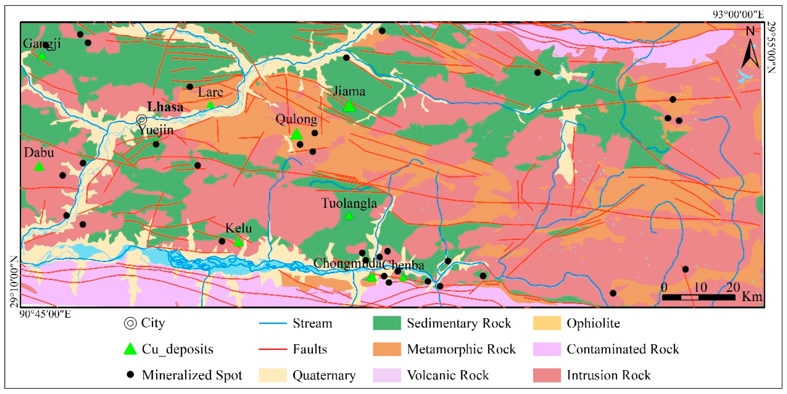
Figure 2.
The ratio of deposit numbers in each stratum to total deposits.
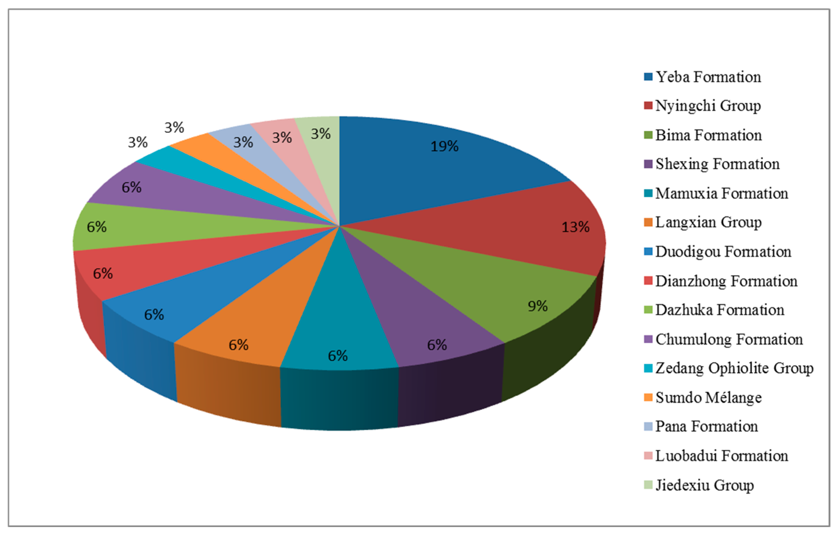
Figure 3.
The stratigraphic combination entropy map.
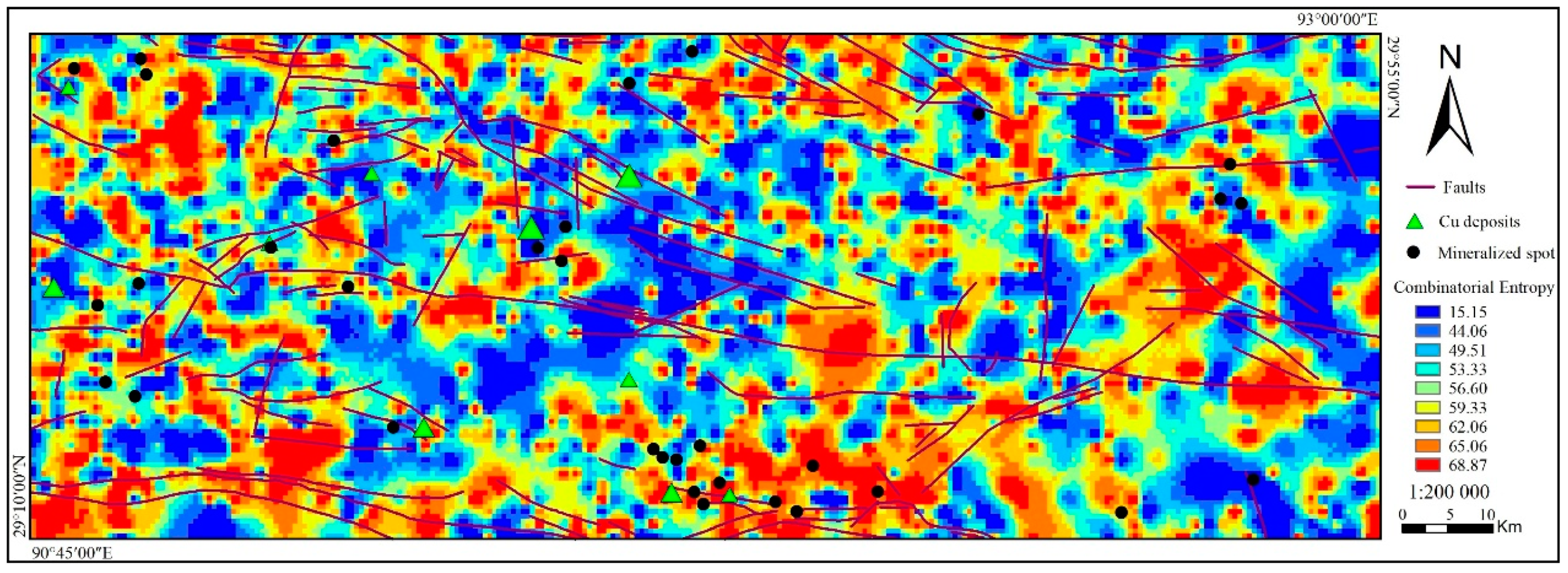
Figure 4.
The structural iso-density map.
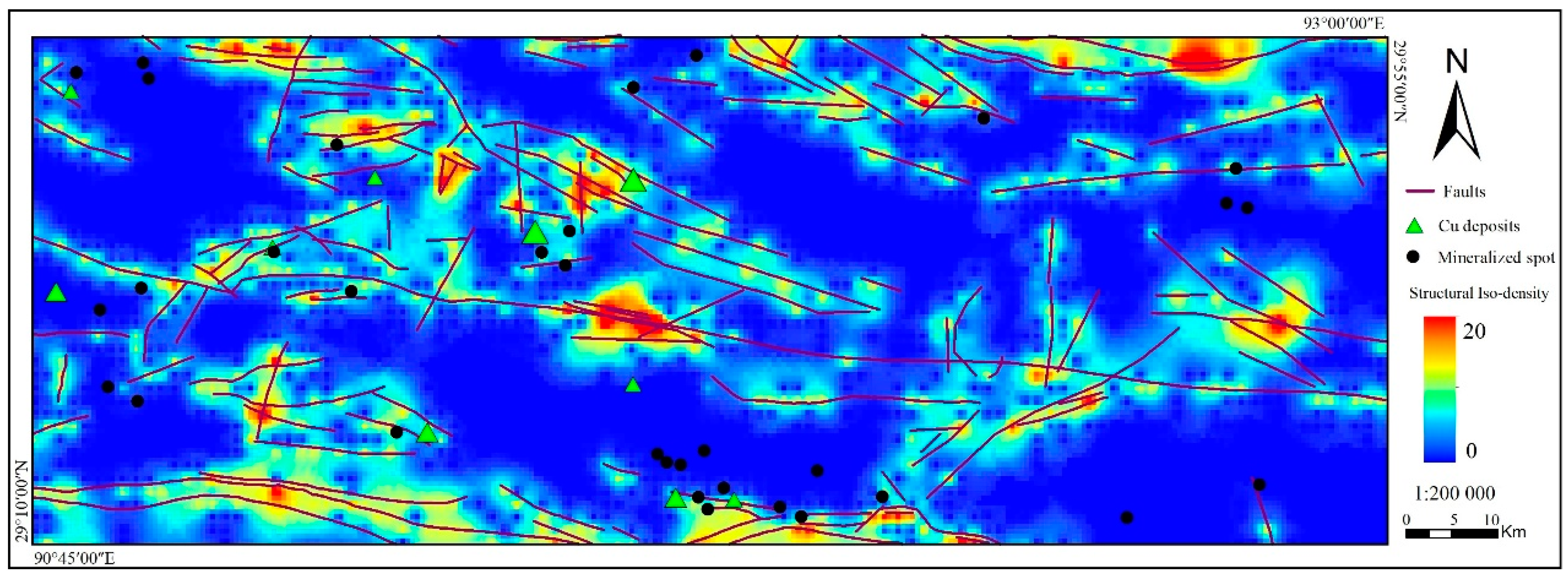
Figure 5.
The structural buffer map.
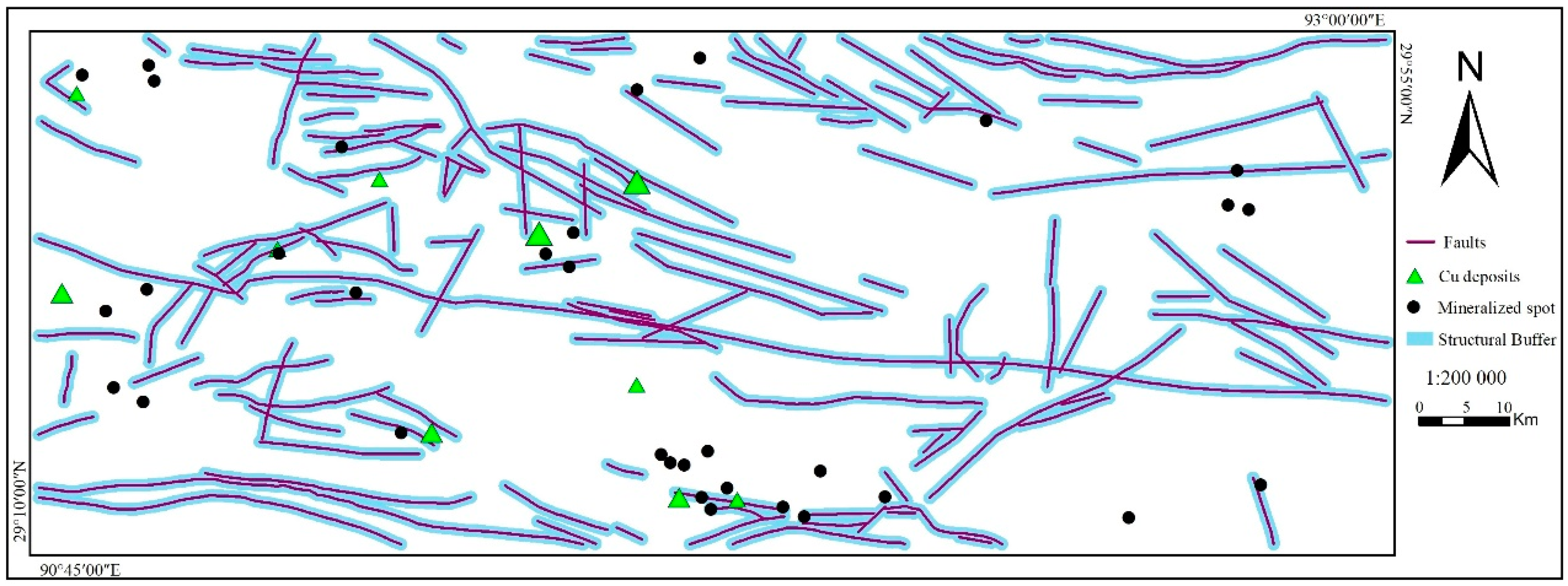
Figure 6.
The regional aeromagnetic ∆T by reduction to the pole based on the vertical first-order derivative map.
Figure 6.
The regional aeromagnetic ∆T by reduction to the pole based on the vertical first-order derivative map.

Figure 7.
Geochemical sampling locations.
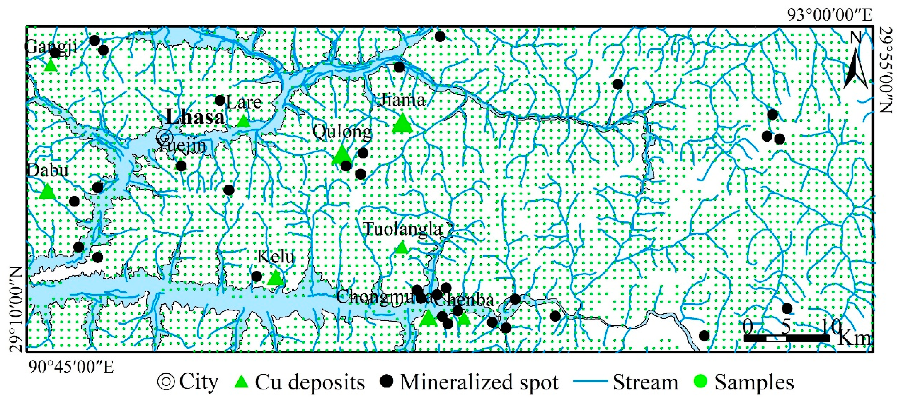
Figure 8.
The distribution of elements Cu (A), Hg (B), La (C), Li (D), Na2O (E), and U (F).
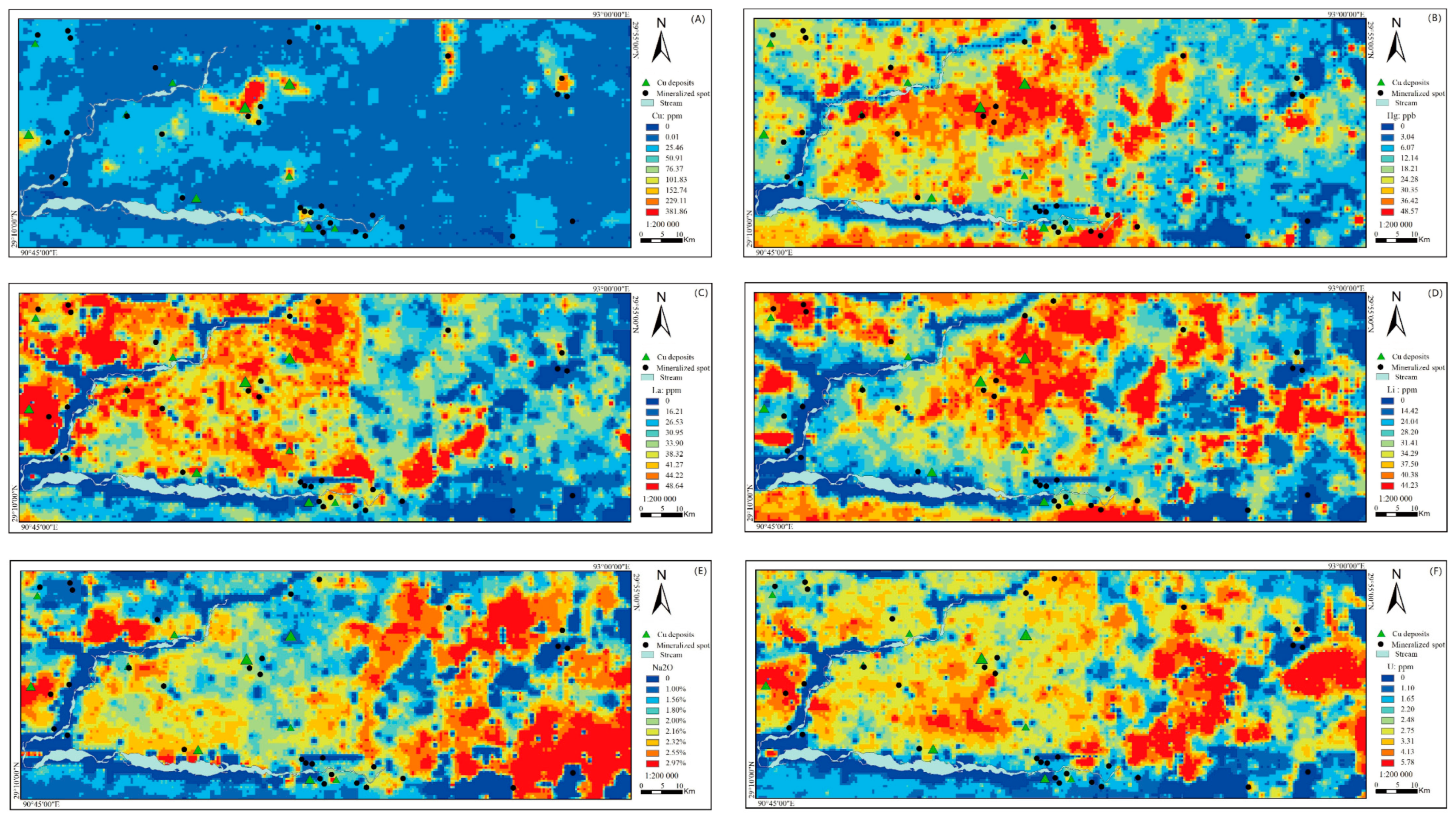
Figure 9.
Jackknife analysis of the individual importance of ore-controlling factors in the MaxEnt model (the green bars show the performance of the global model without each variable; the blue bars show the influence of each variable in isolation; the red bar represents the model results using all variables).
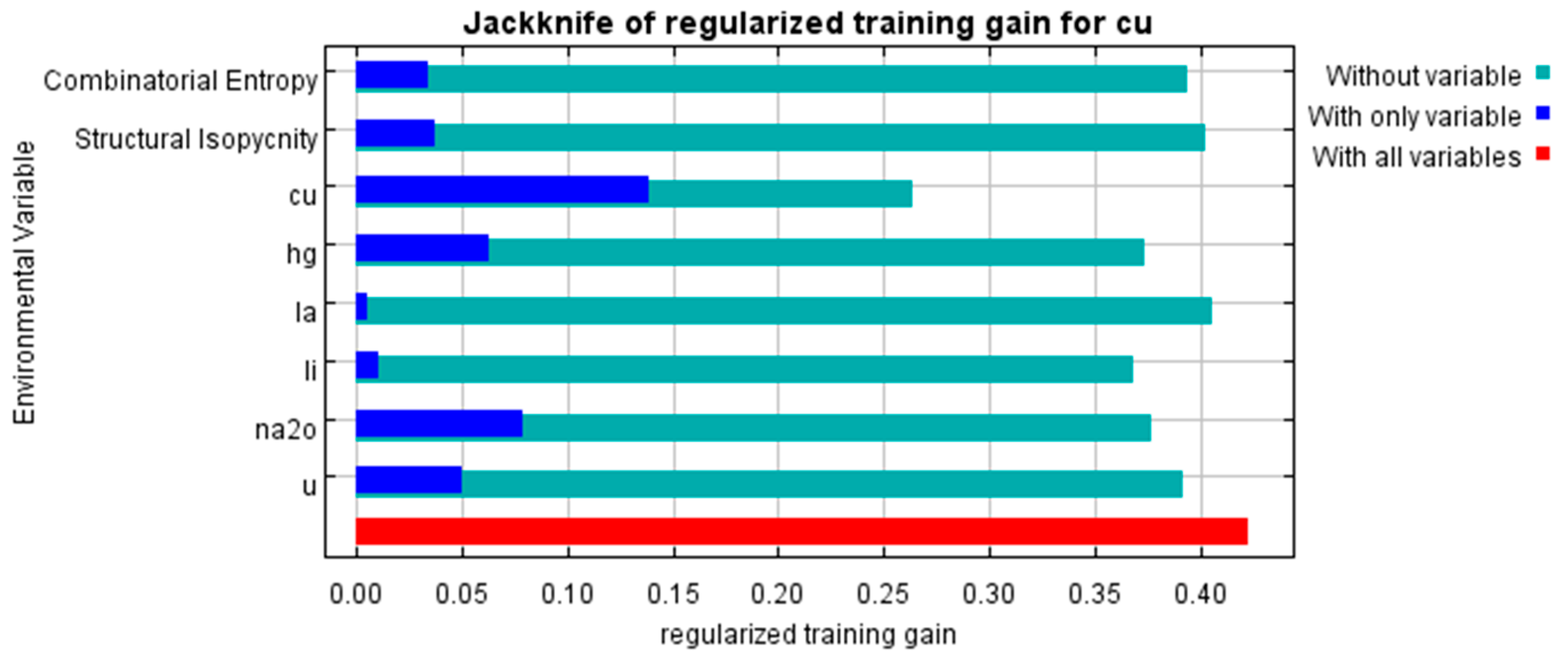
Figure 10.
Response curves of the ore-controlling factors, stratigraphic combination entropy (A); Cu (B); Hg (C); La (D); Li (E); Na2O (F); structural iso-density (G); U (H).
Figure 10.
Response curves of the ore-controlling factors, stratigraphic combination entropy (A); Cu (B); Hg (C); La (D); Li (E); Na2O (F); structural iso-density (G); U (H).
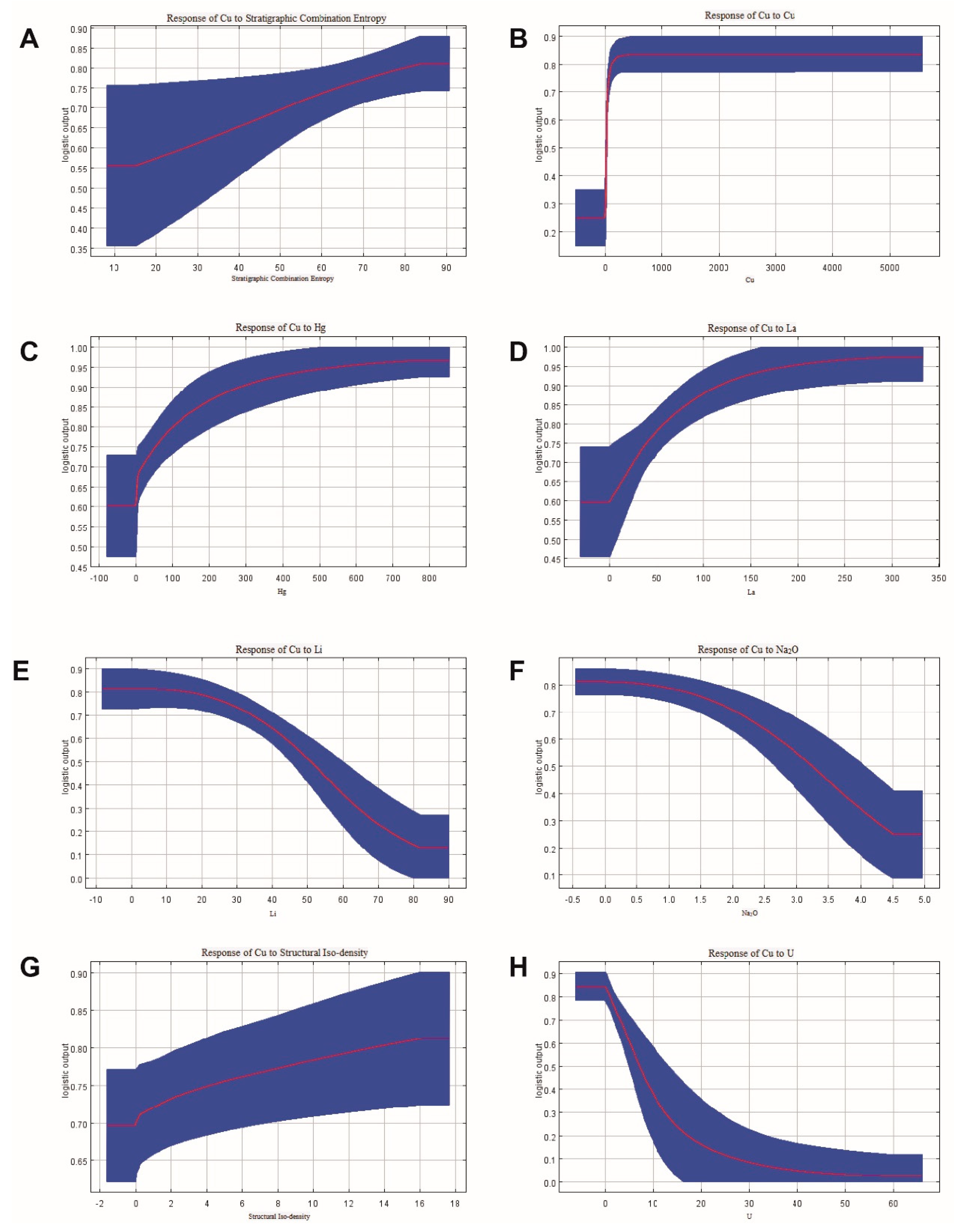
Figure 11.
Continuous-scale copper perspective map of the Mila Mountain generated from the MaxEnt model.
Figure 11.
Continuous-scale copper perspective map of the Mila Mountain generated from the MaxEnt model.
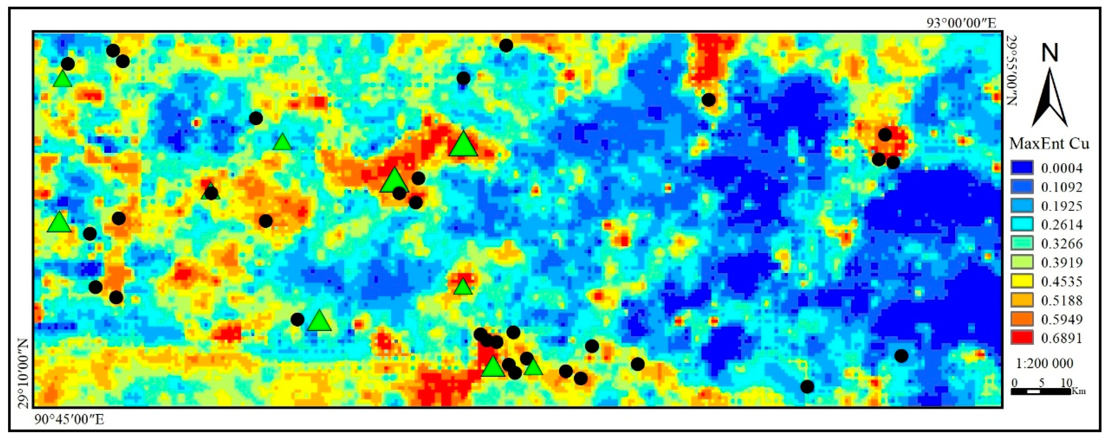
Figure 12.
Binary copper perspective map of the Mila Mountain generated from MaxEnt model.
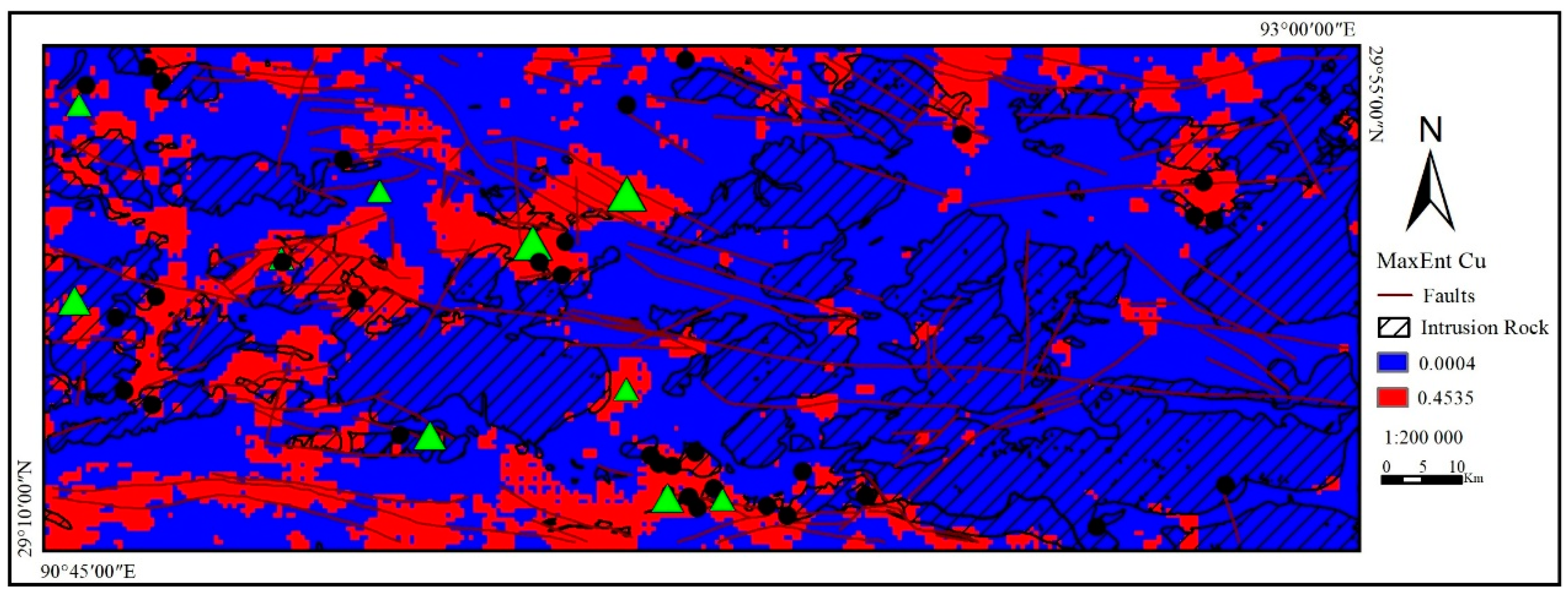
Figure 13.
Prospective area: Areas delineated with rectangles represent targets likely related to mineralization and should be further investigated with more information.
Figure 13.
Prospective area: Areas delineated with rectangles represent targets likely related to mineralization and should be further investigated with more information.

Table 1.
Calculation values of Akaike information criteria (AICc) in each model.
| Model | Variables | Parameters | AICc |
|---|---|---|---|
| 1 | 43 | 53 | - |
| 2 | 15 | 40 | 1401.67 |
| 3 | 10 | 23 | 1155.42 |
| 4 | 43 | 36 | 1301.03 |
| 5 | 9 | 16 | 1125.14 |
| 6 | 8 | 15 | 1120.41 |
| 7 | 43 | 25 | 1175.31 |
| 8 | 9 | 16 | 1128.42 |
| 9 | 43 | 20 | 1149.36 |
| 10 | 10 | 13 | 1121.09 |
| 11 | 9 | 13 | 1123.42 |
| 12 | 43 | 21 | 1159.16 |
| 13 | 10 | 15 | 1131.45 |
| 14 | 8 | 13 | 1125.7 |
| 15 | 7 | 12 | 1122.91 |
Note: “-” indicates that models have more parameters than the sample points, which violate the AICc assumptions, so metrics for these models were not calculated. The “Parameters” represent the number of parameters to be estimated.
Table 2.
The list of training AUC and test AUC.
| No. | Training Samples | Training AUC | Test Samples | Test AUC |
|---|---|---|---|---|
| 1 | 32 | 0.8467 | 11 | 0.8927 |
| 2 | 32 | 0.8468 | 11 | 0.7908 |
| 3 | 32 | 0.8490 | 11 | 0.7277 |
| 4 | 32 | 0.8259 | 11 | 0.7775 |
| 5 | 32 | 0.8033 | 11 | 0.7621 |
| 6 | 32 | 0.8492 | 11 | 0.8027 |
| 7 | 32 | 0.8239 | 11 | 0.8903 |
| 8 | 32 | 0.8733 | 11 | 0.8167 |
| 9 | 32 | 0.8834 | 11 | 0.8258 |
| 10 | 32 | 0.8841 | 11 | 0.6842 |
| 11 | 32 | 0.8664 | 11 | 0.7236 |
| 12 | 32 | 0.8615 | 11 | 0.8225 |
| 13 | 32 | 0.7723 | 11 | 0.7209 |
| 14 | 32 | 0.7938 | 11 | 0.8112 |
| 15 | 32 | 0.8636 | 11 | 0.7549 |
| 16 | 32 | 0.8167 | 11 | 0.8187 |
| 17 | 32 | 0.8369 | 11 | 0.8886 |
| 18 | 32 | 0.8516 | 11 | 0.8952 |
| 19 | 32 | 0.8296 | 11 | 0.7443 |
| 20 | 32 | 0.8497 | 11 | 0.8427 |
| Average | 32 | 0.8414 | 11 | 0.7997 |
Table 3.
The contribution of ore-controlling factors.
| Variable | Percent Contribution | Variable | Percent Contribution |
|---|---|---|---|
| Cu | 38.1% | U | 8.3% |
| Na2O | 15.5% | Combinatorial Entropy | 8% |
| Li | 10.3% | Structural Isopycnity | 7.8% |
| Hg | 10.1% | La | 2.1% |
© 2019 by the authors. Licensee MDPI, Basel, Switzerland. This article is an open access article distributed under the terms and conditions of the Creative Commons Attribution (CC BY) license (http://creativecommons.org/licenses/by/4.0/).
Share and Cite
MDPI and ACS Style
Li, B.; Liu, B.; Guo, K.; Li, C.; Wang, B. Application of a Maximum Entropy Model for Mineral Prospectivity Maps. Minerals 2019, 9, 556. https://doi.org/10.3390/min9090556
AMA Style
Li B, Liu B, Guo K, Li C, Wang B. Application of a Maximum Entropy Model for Mineral Prospectivity Maps. Minerals. 2019; 9(9):556. https://doi.org/10.3390/min9090556
Chicago/Turabian StyleLi, Binbin, Bingli Liu, Ke Guo, Cheng Li, and Bin Wang. 2019. "Application of a Maximum Entropy Model for Mineral Prospectivity Maps" Minerals 9, no. 9: 556. https://doi.org/10.3390/min9090556
Note that from the first issue of 2016, this journal uses article numbers instead of page numbers. See further details here.