Application of a Maximum Entropy Model for Mineral Prospectivity Maps


Abstract
1. Introduction
2. Study Area and Data
2.1. Study Area
2.2. Data
2.2.1. Stratigraphic Combination Entropy
2.2.2. Structural Iso-Density
2.2.3. Structural Buffer
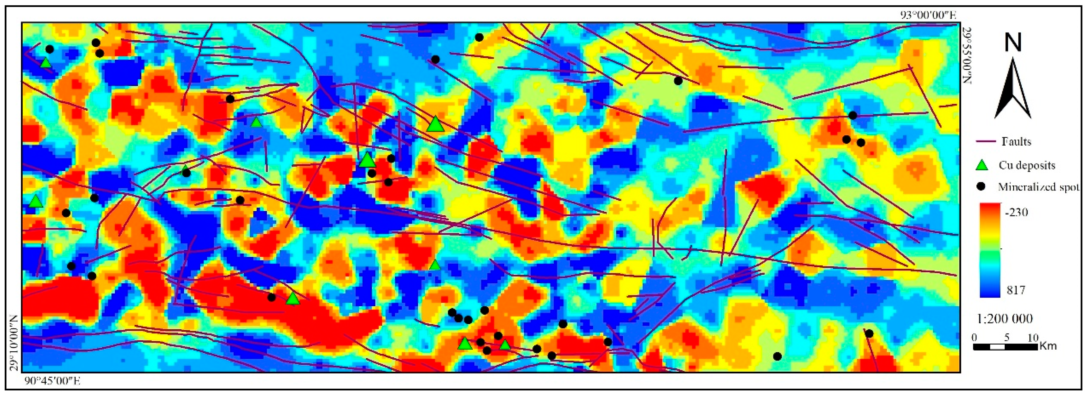
2.2.4. Aeromagnetic Data
2.2.5. Geochemical Data
3. Construction of the Maximum Entropy Model
- (1)
- Enter the selected β value in the MaxEnt software and set the remaining parameters (a maximum of 500 iterations, a maximum convergence threshold of 0.00001, a maximum of 10,000 background points and the replicated run type set to bootstrap) to the default values;
- (2)
- Create a MaxEnt model containing all variables, eliminate the variable with a contribution rate <1%, and eliminate the variable with the Pearson’s correlation coefficient of the highest contribution variable >0.7 to get model 1;
- (3)
- Establish a new MaxEnt model with the remaining variables, eliminate the variables with a contribution rate <1%, and remove the variables with a correlation coefficient of >0.7 with the second highest contribution variable to get model 2;
- (4)
- Repeat the above process until there is no variable with a contribution rate <1%, and get model M;
- (5)
- Change the β value in the MaxEnt software, and set the remaining parameters to the default values; repeat steps 2–4 to obtain a series of MaxEnt models for the distribution of mineral resources;
- (6)
4. Results
4.1. Model Performance Evaluation
4.2. Predictive Variable Contribution
4.3. Response Curves of the Ore-Controlling Factors
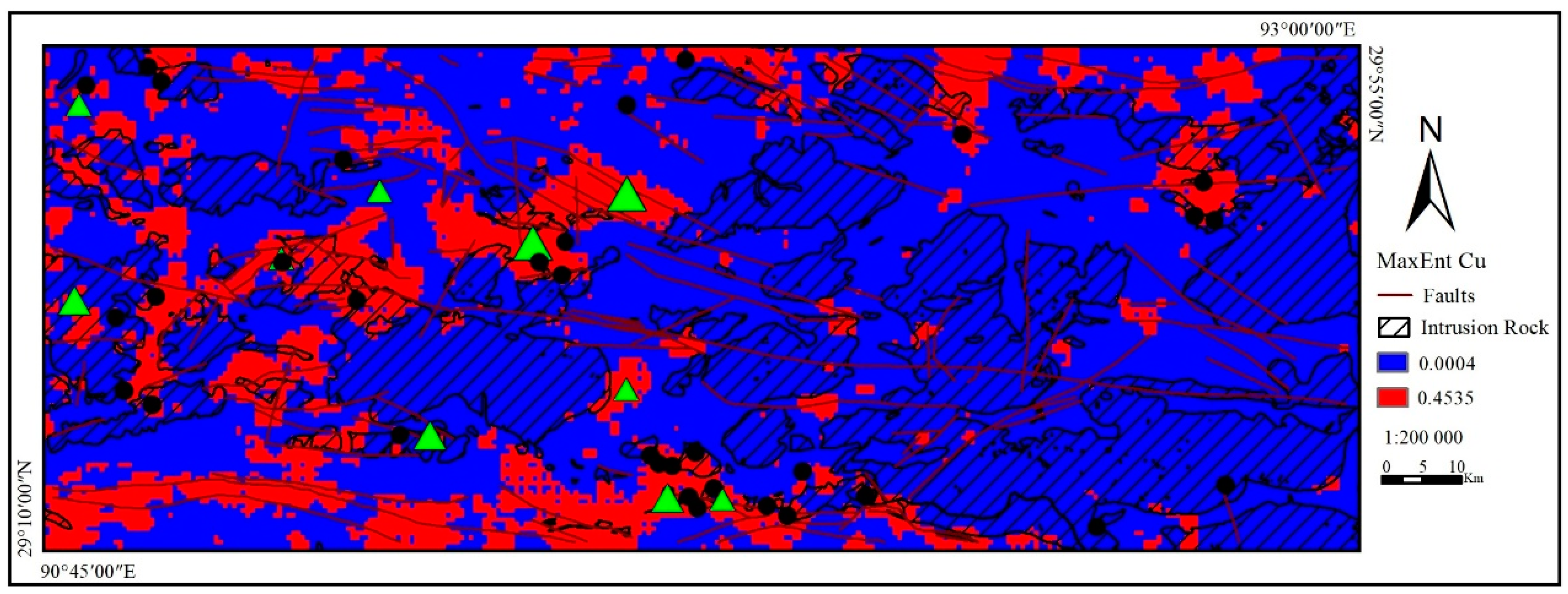
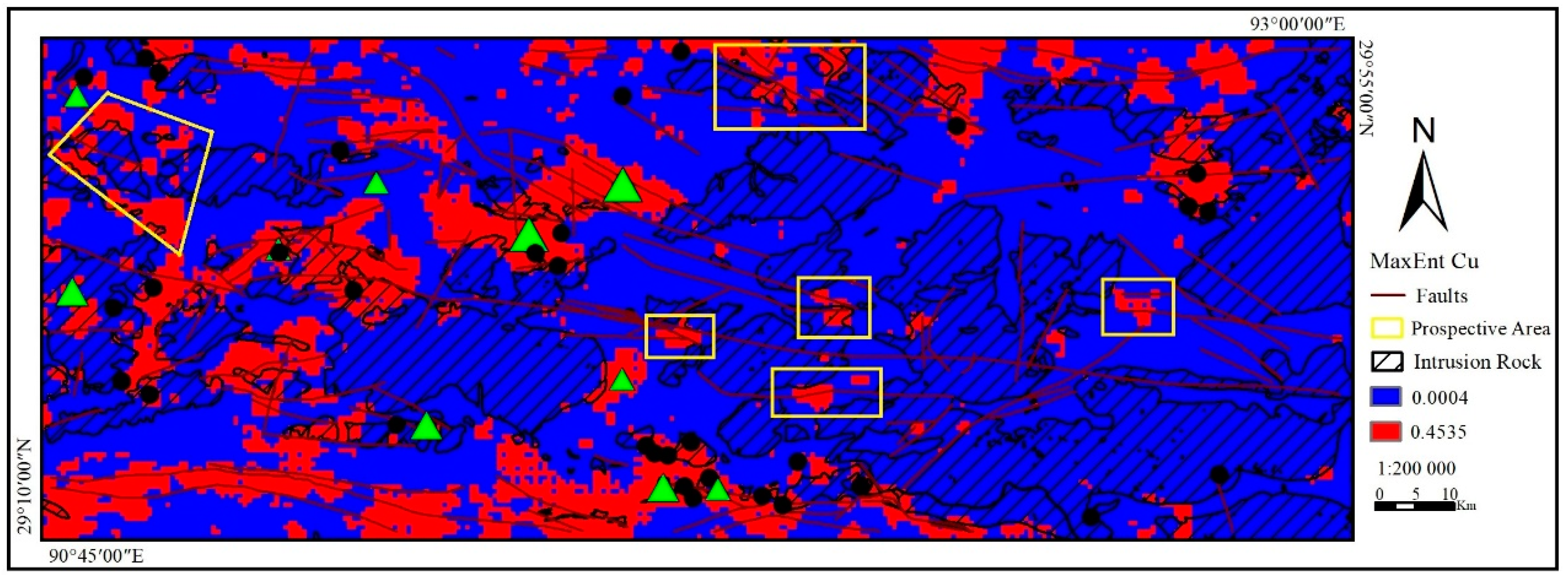
4.4. Perspective Map of Copper
5. Discussion
6. Conclusions
Author Contributions
Funding
Conflicts of Interest
Appendix A

| Factors | β = 2 | β = 2.5 | β = 3 | β = 3.5 | β = 4 | |||||||||||||||||||||||||
|---|---|---|---|---|---|---|---|---|---|---|---|---|---|---|---|---|---|---|---|---|---|---|---|---|---|---|---|---|---|---|
| con | cor | con | cor | con | cor | con | cor | con | cor | con | cor | con | cor | con | cor | con | cor | con | cor | con | cor | con | cor | con | cor | con | cor | con | cor | |
| Model | 1 | 1 | 2 | 2 | 3 | 3 | 4 | 4 | 5 | 5 | 6 | 6 | 7 | 7 | 8 | 8 | 9 | 9 | 10 | 10 | 11 | 11 | 12 | 12 | 13 | 13 | 14 | 14 | 15 | 15 |
| Cu | 45.80 | 1.00 | 46.20 | 0.04 | 51.80 | 0.01 | 47.60 | 1.00 | 54.00 | 0.04 | 51.50 | 0.01 | 45.50 | 1.00 | 48.00 | 0.04 | 42.20 | 1.00 | 42.80 | 0.04 | 41.20 | 0.11 | 44.10 | 1.00 | 43.80 | 0.04 | 44.90 | 0.11 | 44.10 | 0.11 |
| Na2O | 16.20 | 0.04 | 17.80 | 1.00 | 18.20 | −0.01 | 16.40 | 0.04 | 16.40 | 1.00 | 18.80 | 0.32 | 20.70 | 0.04 | 20.50 | 1.00 | 26.20 | 0.04 | 27.60 | 1.00 | 27.30 | 0.40 | 28.60 | 0.04 | 29.00 | 1.00 | 30.00 | 0.40 | 29.70 | 0.10 |
| Li | 3.70 | 0.11 | 4.80 | 0.40 | 4.70 | 0.30 | 6.20 | 0.11 | 7.60 | 0.40 | 9.30 | 0.30 | 10.60 | 0.11 | 11.90 | 0.40 | 7.00 | 0.11 | 8.70 | 0.40 | 12.80 | 1.00 | 7.40 | 0.11 | 10.40 | 0.40 | 10.40 | 1.00 | 10.10 | 0.15 |
| W | 1.10 | 0.11 | 0.40 | - | - | - | 0.90 | - | - | - | - | - | 3.30 | 0.11 | 3.70 | 0.10 | 3.50 | 0.11 | 4.90 | 0.10 | 4.30 | 0.15 | 5.60 | 0.11 | 5.60 | 0.10 | 5.80 | 0.15 | 5.70 | 1.00 |
| Structural Iso-density | 1.60 | 0.02 | 3.80 | −0.01 | 2.80 | −0.06 | 3.50 | 0.02 | 3.50 | −0.05 | 2.90 | −0.07 | 2.50 | 0.02 | 2.60 | −0.05 | 4.20 | 0.02 | 4.30 | −0.05 | 4.10 | 0.15 | 4.10 | 0.02 | 4.20 | −0.05 | 4.50 | 0.15 | 4.50 | −0.02 |
| SiO2 | 2.40 | 0.08 | 0.20 | - | - | - | 0.00 | - | - | - | - | - | 0.00 | - | - | - | 3.20 | 0.08 | 1.20 | 0.73 | - | - | 2.50 | 0.08 | 0.00 | - | - | - | - | - |
| U | 10.30 | 0.01 | 10.40 | 0.32 | 8.90 | 1.00 | 10.10 | 0.01 | 9.00 | 0.32 | 8.70 | 1.00 | 7.00 | 0.01 | 5.90 | 0.32 | 5.60 | 0.01 | 5.20 | 0.32 | 5.30 | 0.30 | 2.40 | 0.01 | 2.80 | 0.32 | 1.20 | 0.30 | 1.40 | 0.15 |
| Hg | 3.20 | 0.09 | 3.90 | 0.06 | 3.50 | 0.09 | 4.00 | 0.09 | 5.00 | 0.06 | 4.60 | 0.09 | 3.80 | 0.09 | 3.70 | 0.06 | 3.70 | 0.09 | 2.20 | 0.06 | 2.30 | 0.42 | 1.40 | 0.09 | 2.10 | 0.06 | 2.30 | 0.42 | 4.50 | 0.09 |
| La | 1.70 | 0.14 | 1.50 | 0.50 | 1.80 | 0.37 | 2.00 | 0.14 | 1.80 | 0.50 | 1.90 | 0.37 | 1.70 | 0.14 | 1.50 | 0.50 | 1.50 | 0.14 | 1.30 | 0.50 | 1.20 | 0.62 | 1.00 | 0.14 | 0.90 | - | - | - | - | - |
| Combinatorial Entropy | 1.70 | −0.02 | 2.00 | 0.01 | 2.20 | −0.02 | 2.50 | −0.02 | 2.60 | 0.01 | 2.30 | −0.02 | 2.10 | −0.02 | 2.30 | 0.01 | 1.80 | −0.02 | 1.90 | 0.01 | 1.60 | 0.04 | 1.00 | −0.02 | 1.20 | 0.01 | 0.90 | - | - | - |
| Mo | 1.10 | 0.27 | 1.50 | 0.09 | 3.50 | 0.22 | 0.60 | - | - | - | - | - | 0.20 | - | - | - | 0.00 | - | - | - | - | - | 0.90 | - | - | - | - | - | - | - |
| Cr | 0.00 | - | - | - | - | - | 0.20 | - | - | - | - | - | 0.50 | - | - | - | 0.00 | - | - | - | - | - | 0.70 | - | - | - | - | - | - | - |
| Aeromagnetic Data | 0.90 | - | - | - | - | - | 0.80 | - | - | - | - | - | 0.60 | - | - | - | 0.50 | - | - | - | - | - | 0.30 | - | - | - | - | - | - | - |
| Sb | 1.70 | 0.13 | 0.30 | - | - | - | 0.70 | - | - | - | - | - | 0.10 | - | - | - | 0.00 | - | - | - | - | - | 0.10 | - | - | - | - | - | - | - |
| Ag | 0.10 | - | - | - | - | - | 0.10 | - | - | - | - | - | 0.00 | - | - | - | 0.00 | - | - | - | - | - | 0.00 | - | - | - | - | - | - | - |
| Al2O3 | 0.00 | - | - | - | - | - | 0.00 | - | - | - | - | - | 0.00 | - | - | - | 0.00 | - | - | - | - | - | 0.00 | - | - | - | - | - | - | - |
| As | 0.10 | - | - | - | - | - | 0.10 | - | - | - | - | - | 0.00 | - | - | - | 0.00 | - | - | - | - | - | 0.00 | - | - | - | - | - | - | - |
| Au | 0.00 | - | - | - | - | - | 0.00 | - | - | - | - | - | 0.00 | - | - | - | 0.00 | - | - | - | - | - | 0.00 | - | - | - | - | - | - | - |
| B | 0.00 | - | - | - | - | - | 0.00 | - | - | - | - | - | 0.00 | - | - | - | 0.00 | - | - | - | - | - | 0.00 | - | - | - | - | - | - | - |
| Ba | 0.10 | - | - | - | - | - | 0.00 | - | - | - | - | - | 0.00 | - | - | - | 0.00 | - | - | - | - | - | 0.00 | - | - | - | - | - | - | - |
| Be | 0.00 | - | - | - | - | - | 0.00 | - | - | - | - | - | 0.00 | - | - | - | 0.00 | - | - | - | - | - | 0.00 | - | - | - | - | - | - | - |
| Bi | 0.10 | - | - | - | - | - | 0.00 | - | - | - | - | - | 0.00 | - | - | - | 0.00 | - | - | - | - | - | 0.00 | - | - | - | - | - | - | - |
| CaO | 1.10 | 0.05 | 0.20 | - | - | - | 0.80 | - | - | - | - | - | 0.30 | - | - | - | 0.00 | - | - | - | - | - | 0.00 | - | - | - | - | - | - | - |
| Cd | 0.20 | - | - | - | - | - | 0.00 | - | - | - | - | - | 0.00 | - | - | - | 0.00 | - | - | - | - | - | 0.00 | - | - | - | - | - | - | - |
| Co | 0.00 | - | - | - | - | - | 0.00 | - | - | - | - | - | 0.00 | - | - | - | 0.00 | - | - | - | - | - | 0.00 | - | - | - | - | - | - | - |
| Structural Buffer | 1.00 | 0.05 | 0.70 | - | - | - | 0.20 | - | - | - | - | - | 0.00 | - | - | - | 0.00 | - | - | - | - | - | 0.00 | - | - | - | - | - | - | - |
| F | 0.00 | - | - | - | - | - | 0.00 | - | - | - | - | - | 0.00 | - | - | - | 0.00 | - | - | - | - | - | 0.00 | - | - | - | - | - | - | - |
| Fe2O3 | 0.00 | - | - | - | - | - | 0.00 | - | - | - | - | - | 0.00 | - | - | - | 0.00 | - | - | - | - | - | 0.00 | - | - | - | - | - | - | - |
| K2O | 0.00 | - | - | - | - | - | 0.00 | - | - | - | - | - | 0.00 | - | - | - | 0.00 | - | - | - | - | - | 0.00 | - | - | - | - | - | - | - |
| MgO | 0.00 | - | - | - | - | - | 0.00 | - | - | - | - | - | 0.00 | - | - | - | 0.00 | - | - | - | - | - | 0.00 | - | - | - | - | - | - | - |
| Mn | 0.00 | - | - | - | - | - | 0.00 | - | - | - | - | - | 0.00 | - | - | - | 0.00 | - | - | - | - | - | 0.00 | - | - | - | - | - | - | - |
| Nb | 0.60 | - | - | - | - | - | 0.50 | - | - | - | - | - | 0.30 | - | - | - | 0.00 | - | - | - | - | - | 0.00 | - | - | - | - | - | - | - |
| Ni | 0.80 | - | - | - | - | - | 0.00 | - | - | - | - | - | 0.00 | - | - | - | 0.00 | - | - | - | - | - | 0.00 | - | - | - | - | - | - | - |
| pb | 0.00 | - | - | - | - | - | 0.80 | - | - | - | - | - | 0.50 | - | - | - | 0.20 | - | - | - | - | - | 0.00 | - | - | - | - | - | - | - |
| Pb | 0.00 | - | - | - | - | - | 0.00 | - | - | - | - | - | 0.00 | - | - | - | 0.00 | - | - | - | - | - | 0.00 | - | - | - | - | - | - | - |
| Sn | 0.00 | - | - | - | - | - | 0.00 | - | - | - | - | - | 0.00 | - | - | - | 0.00 | - | - | - | - | - | 0.00 | - | - | - | - | - | - | - |
| Sr | 0.10 | - | - | - | - | - | 0.10 | - | - | - | - | - | 0.00 | - | - | - | 0.00 | - | - | - | - | - | 0.00 | - | - | - | - | - | - | - |
| Th | 0.00 | - | - | - | - | - | 0.00 | - | - | - | - | - | 0.00 | - | - | - | 0.00 | - | - | - | - | - | 0.00 | - | - | - | - | - | - | - |
| Ti | 0.20 | - | - | - | - | - | 0.00 | - | - | - | - | - | 0.00 | - | - | - | 0.00 | - | - | - | - | - | 0.00 | - | - | - | - | - | - | - |
| V | 0.00 | - | - | - | - | - | 0.00 | - | - | - | - | - | 0.00 | - | - | - | 0.00 | - | - | - | - | - | 0.00 | - | - | - | - | - | - | - |
| Y | 0.50 | - | - | - | - | - | 0.60 | - | - | - | - | - | 0.30 | - | - | - | 0.20 | - | - | - | - | - | 0.00 | - | - | - | - | - | - | - |
| Zn | 2.40 | 0.26 | 6.30 | 0.17 | 2.60 | 0.16 | 1.40 | 0.26 | 0.20 | - | - | - | 0.00 | - | - | - | 0.00 | - | - | - | - | - | 0.00 | - | - | - | - | - | - | - |
| Zr | 0.50 | - | - | - | - | - | 0.00 | - | - | - | - | - | 0.00 | - | - | - | 0.00 | - | - | - | - | - | 0.00 | - | - | - | - | - | - | - |
References
- Harris, D.P. An Application of Multivariate Statistical Analysis to Mineral Exploration. Ph.D. Thesis, The Pennsylvania State University, State College, PA, USA, 1965. [Google Scholar]
- Agterberg, F. Automatic contouring of geological maps to detect target areas for mineral exploration. Math. Geol. 1974, 6, 373–395. [Google Scholar] [CrossRef]
- Bonham-Carter, G.F. Geographic Information Systems for Geoscientists: Modelling with GIS; Elsevier: Amsterdam, The Netherlands, 1994; Volume 13, p. 416. [Google Scholar]
- An, P.; Moon, W.; Rencz, A. Application of fuzzy set theory for integration of geological, geophysical and remote sensing data. Can. J. Explor. Geophys. 1991, 27, 1–11. [Google Scholar]
- Ford, A.; Miller, J.M.; Mol, A.G. A comparative analysis of weights of evidence, evidential belief functions, and fuzzy logic for mineral potential mapping using incomplete data at the scale of investigation. Nat. Resour. Res. 2016, 25, 19–33. [Google Scholar] [CrossRef]
- Carranza, E.J.M.; Mangaoang, J.C.; Hale, M. Application of mineral exploration models and GIS to generate mineral potential maps as input for optimum land-use planning in the Philippines. Nat. Resour. Res. 1999, 8, 165–173. [Google Scholar] [CrossRef]
- An, P.; Moon, W.; Bonham-Carter, G. Uncertainty management in integration of exploration data using the belief function. Nonrenew. Res. 1994, 3, 60–71. [Google Scholar] [CrossRef]
- Carranza, E.; Woldai, T.; Chikambwe, E. Application of data-driven evidential belief functions to prospectivity mapping for aquamarine-bearing pegmatites, Lundazi district, Zambia. Nat. Resour. Res. 2005, 14, 47–63. [Google Scholar] [CrossRef]
- Carranza, E.J.M. Geochemical Anomaly and Mineral Prospectivity Mapping in GIS; Elsevier: Amsterdam, The Netherlands, 2008; Volume 11, p. 365. [Google Scholar]
- Carranza, E.J.M. Improved wildcat modelling of mineral prospectivity. Resour. Geol. 2010, 60, 129–149. [Google Scholar] [CrossRef]
- Carranza, E.; Hale, M. Wildcat mapping of gold potential, Baguio district, Philippines. Appl. Earth Sci. 2002, 111, 100–105. [Google Scholar] [CrossRef]
- Grunsky, E.; Agterberg, F. The application of spatial factor analysis to unconditional simulations with implications for mineral exploration. In Proceedings of the 21st International Symposium on Computers in the Mineral Industry; Society of Mining Engineers of AIME: Las Vegas, NV, USA, 1989; pp. 194–208. [Google Scholar]
- Agterberg, F.P. Combining indicator patterns in weights of evidence modeling for resource evaluation. Nonrenew. Res. 1992, 1, 39–50. [Google Scholar] [CrossRef]
- Bonham-Carter, G.F. Weights of evidence modeling: A new approach to mapping mineral potential. Stat. Appl. Earth Sci. 1989, 98, 171–183. [Google Scholar]
- Liu, Y.; Cheng, Q.; Xia, Q.; Wang, X. Mineral potential mapping for tungsten polymetallic deposits in the Nanling metallogenic belt, South China. J. Earth Sci. 2014, 25, 689–700. [Google Scholar] [CrossRef]
- Ziaii, M.; Pouyan, A.; Ziaei, M. A computational optimized extended model for mineral potential mapping based on W of E method. Am. J. Appl. Sci. 2009, 6, 200–203. [Google Scholar]
- Cheng, Q.; Chen, Z.; Khaled, A. Application of fuzzy weights of evidence method in mineral resource assessment for gold in Zhenyuan District, Yunnan Province, China. Earth Sci. 2007, 32, 175–184. [Google Scholar]
- Agterberg, F.; Bonham-Carter, G. Logistic regression and weights of evidence modeling in mineral exploration. In Proceedings of the 28th International Symposium on Applications of Computer in the Mineral Industry (APCOM), Golden, CO, USA, 20–22 October 1999; p. 490. [Google Scholar]
- Carranza, E.; Hale, M.; Faassen, C. Selection of coherent deposit-type locations and their application in data-driven mineral prospectivity mapping. Ore Geol. Rev. 2008, 33, 536–558. [Google Scholar] [CrossRef]
- Chen, C.; Dai, H.; Liu, Y.; He, B. Mineral prospectivity mapping integrating multi-source geology spatial data sets and logistic regression modelling. In Proceedings of the 2011 IEEE International Conference on Spatial Data Mining and Geographical Knowledge Services, Fuzhou, China, 29 June–1 July 2011; pp. 214–217. [Google Scholar]
- Brown, W.M.; Gedeon, T.; Groves, D.; Barnes, R. Artificial neural networks: A new method for mineral prospectivity mapping. Aust. J. Earth Sci. 2000, 47, 757–770. [Google Scholar] [CrossRef]
- Skabar, A. Mineral potential mapping using feed-forward neural networks. In Proceedings of the International Joint Conference on Neural Networks, Portland, OR, USA, 20–24 July 2003; pp. 1814–1819. [Google Scholar]
- Leite, E.P.; de Souza Filho, C.R. Artificial neural networks applied to mineral potential mapping for copper-gold mineralizations in the Carajás Mineral Province, Brazil. Geophys. Prospect. 2009, 57, 1049–1065. [Google Scholar] [CrossRef]
- Leite, E.P.; de Souza Filho, C.R. Probabilistic neural networks applied to mineral potential mapping for platinum group elements in the Serra Leste region, Carajás Mineral Province, Brazil. Comput. Geosci. 2009, 35, 675–687. [Google Scholar] [CrossRef]
- Oh, H.-J.; Lee, S. Application of artificial neural network for gold–silver deposits potential mapping: A case study of Korea. Nat. Resour. Res. 2010, 19, 103–124. [Google Scholar] [CrossRef]
- Cheng, Q.M. Singularity-generalized self-similarity-fractal spectrum (3S) models. Earth Sci. 2006, 31, 337–348. [Google Scholar]
- Cheng, Q.M.; Zhao, P.D.; Chen, J.G.; Xia, Q.L.; Chen, Z.J.; Zhan, S.Y.; Xu, D.Y.; Xia, X.Y.; Wan, W.L. Application of singularity theory in prediction of tin and copper mineral deposits in Gejiu district, Yunnan, China: Weak information extraction and mixing information decomposition. Earth Sci. 2009, 34, 243–252. [Google Scholar]
- Liu, B.; Guo, K.; Li, C.; Zhou, J.; Liu, X.; Wang, X.; Wang, L. Copper prospectivity in Tibet, China: Based on the identification of geochemical anomalies. Ore Geol. Rev. 2018. [Google Scholar] [CrossRef]
- Abedi, M.; Norouzi, G.H.; Bahroudi, A. Support vector machine for multi-classification of mineral prospectivity areas. Comput. Geosci. 2012, 46, 272–283. [Google Scholar] [CrossRef]
- Zuo, R.; Carranza, E.J.M. Support vector machine: A tool for mapping mineral prospectivity. Comput. Geosci. 2011, 37, 1967–1975. [Google Scholar] [CrossRef]
- Geranian, H.; Tabatabaei, S.H.; Asadi, H.H.; Carranza, E.J.M. Application of discriminant analysis and support vector machine in mapping gold potential areas for further drilling in the Sari-Gunay gold deposit, NW Iran. Nat. Resour. Res. 2016, 25, 145–159. [Google Scholar] [CrossRef]
- Rodriguez-Galiano, V.F.; Chica-Olmo, M.; Chica-Rivas, M. Predictive modelling of gold potential with the integration of multisource information based on random forest: A case study on the Rodalquilar area, Southern Spain. Int. J. Geogr. Inf. Sci. 2014, 28, 1336–1354. [Google Scholar] [CrossRef]
- Carranza, E.J.M.; Laborte, A.G. Random forest predictive modeling of mineral prospectivity with small number of prospects and data with missing values in Abra (Philippines). Comput. Geosci. 2015, 74, 60–70. [Google Scholar] [CrossRef]
- Yuan, G.; Zhang, Z.; Xiong, Y.; Zuo, R. Mapping mineral prospectivity for Cu polymetallic mineralization in southwest Fujian Province, China. Ore Geol. Rev. 2016, 75, 16–28. [Google Scholar]
- Cheng, Q.; Agterberg, F.P. Fuzzy weights of evidence method and its application in mineral potential mapping. Nat. Resour. Res. 1999, 8, 27–35. [Google Scholar] [CrossRef]
- Porwal, A.; Carranza, E.J.M.; Hale, M. A hybrid neuro-fuzzy model for mineral potential mapping. Math. Geol. 2004, 36, 803–826. [Google Scholar] [CrossRef]
- Porwal, A.; Carranza, E.J.M.; Hale, M. A hybrid fuzzy weights-of-evidence model for mineral potential mapping. Nat. Resour. Res. 2006, 15, 1–14. [Google Scholar] [CrossRef]
- Phillips, S.J.; Anderson, R.P.; Schapire, R.E. Maximum entropy modeling of species geographic distributions. Ecol. Model. 2006, 190, 231–259. [Google Scholar] [CrossRef]
- Phillips, S.J.; Jane, E. On estimating probability of presence from use-availability or presence-background data. Ecology 2013, 94, 1409–1419. [Google Scholar] [CrossRef] [PubMed]
- Berger, A.L.; Pietra, V.J.D.; Pietra, S.A.D. A maximum entropy approach to natural language processing. Comput. Linguist. 2002, 22, 39–71. [Google Scholar]
- Dong, Y.; Hinton, G.E.; Morgan, N.; Chien, J.T.; Sagayama, S. Introduction to the special section on deep learning for speech and language processing. IEEE Trans. Audio Speech 2012, 20, 4–6. [Google Scholar]
- Xu, Y.; Wu, Z.; Long, J.; Song, X. A maximum entropy method for a robust portfolio problem. Entropy 2014, 16, 3401–3415. [Google Scholar] [CrossRef]
- Wang, B.; Xu, Y.; Ran, J. Predicting suitable habitat of the Chinese monal (Lophophorus lhuysii) using ecological niche modeling in the Qionglai Mountains, China. PeerJ 2017, 5, e3477. [Google Scholar] [CrossRef]
- Liu, Y.; Zhou, K.; Zhang, N.; Wang, J. Maximum entropy modeling for orogenic gold prospectivity mapping in the Tangbale-Hatu belt, western Junggar, China. Ore Geol. Rev. 2018, 100, 133–147. [Google Scholar] [CrossRef]
- Song, Y.; Yang, C.; Wei, S.; Yang, H.; Fang, X.; Lu, H. Tectonic control, reconstruction and preservation of the Tiegelongnan porphyry and epithermal overprinting Cu (Au) deposit, central Tibet, China. Minerals 2018, 8, 398. [Google Scholar] [CrossRef]
- Lin, B.; Tang, J.X.; Chen, Y.C.; Song, Y.; Hall, G.; Wang, Q.; Yang, C.; Fang, X.; Duan, J.L.; Yang, H.H. Geochronology and genesis of the Tiegelongnan Porphyry Cu (Au) deposit in Tibet: Evidence from U–Pb, Re–Os Dating and Hf, S., and H–O isotopes. Resour. Geol. 2017, 67, 1–21. [Google Scholar] [CrossRef]
- Lin, B.; Chen, Y.; Tang, J.; Wang, Q.; Song, Y.; Yang, C.; Wang, W.; He, W.; Zhang, L. 40Ar/39Ar and Rb-Sr ages of the Tiegelongnan Porphyry Cu-(Au) Deposit in the Bangong Co-Nujiang Metallogenic Belt of Tibet, China: Implication for generation of super-large deposit. Acta Geol. Sin. 2017, 91, 602–616. [Google Scholar] [CrossRef]
- Lin, B.; Tang, J.; Chen, Y.; Baker, M.; Song, Y.; Yang, H.; Wang, Q.; He, W.; Liu, Z. Geology and geochronology of Naruo large porphyry-breccia Cu deposit in the Duolong district, Tibet. Gondwana Res. 2019, 66, 168–182. [Google Scholar] [CrossRef]
- Cheng, W.B.; Gu, X.X.; Tang, J.X.; Wang, L.Q.; Lv, P.R.; Zhong, K.H.; Liu, X.J.; Gao, Y.M. Lead isotope characteristics of ore sulfides from typical deposits in the Gangdese-Nyainqentanglha metallogenic belt Implications for the zonation of ore forming elements. Acta Petrol. Sin. 2010, 26, 3350–3362. [Google Scholar]
- Xie, J.C.; Li, W.K.; Dong, G.C.; Mo, X.X.; Zhao, Z.D.; Yu, J.C.; Wang, T.C. Petrology, geochemistry and tectonic significance of the granites from Basu area, Tibet. Acta Petrol. Sin. 2013, 29, 3779–3791. [Google Scholar]
- Lang, X.H.; Tang, J.X.; Chen, Y.C.; Li, Z.J.; Huang, Y.; Wang, C.H. Neo-Tethys mineralization on the southern margin of the Gangdise Metallogenic Belt, Tibet, China: Evidence from Re-Os ages of Xiongcun orebody No. I. Earth Sci. 2012, 37, 515–525. [Google Scholar]
- Leng, C.-B.; Zhang, X.-C.; Zhong, H.; Hu, R.-Z.; Zhou, W.-D.; Li, C. Re–Os molybdenite ages and zircon Hf isotopes of the Gangjiang porphyry Cu–Mo deposit in the Tibetan Orogen. Miner. Depos. 2013, 48, 585–602. [Google Scholar] [CrossRef]
- Yin, A.; Harrison, T.M. Geologic evolution of the Himalayan-Tibetan orogen. Annu. Rev. Earth. Planet. Sci. 2000, 28, 211–280. [Google Scholar] [CrossRef]
- Zheng, W.; Tang, J.; Zhong, K.; Ying, L.; Leng, Q.; Ding, S.; Lin, B. Geology of the Jiama porphyry copper–polymetallic system, Lhasa Region, China. Ore Geol. Rev. 2016, 74, 151–169. [Google Scholar] [CrossRef]
- Yang, Z.M.; Hou, Z.Q. Genesis of giant porphyry Cu deposit at Qulong, Tibet: Constraints from fluid inclusions and H-O isotopes. Acta Geol. Sin. 2009, 83, 1838–1859. [Google Scholar]
- Chi Shundu, Z.P. Application of combined-entropy anomaly of geological formations to delineation of preferable ore-finding area. Geo. Scine. Ce. 2000, 14, 423–428. [Google Scholar]
- Zhao Buyi, Q.X. Quantitative analysis method of remote sensing structure. Geol. Sci. Technol. Inf. 1988, 7, 127–136. [Google Scholar]
- Sun Xiang, Z.Z.; Yang, Z. Extraction of geological anomaly and delineation of preferable ore-finding area based on MAPGIS. J. Liaon. Tech. Univ. 2007, 26, 837–840. [Google Scholar]
- Dong, Q.J.; Xiao, K.Y.; Chen, J.P.; Cong, Y. The quantitative analysis of regional metallogenic fault in the northern segment of the Sanjiang metallogenic belt, southwestern China. Geol. Bull. China 2010, 29, 1479–1485. [Google Scholar]
- Jiang, S.L.Y.; Feng, J.; Li, L.; Yuan, H.; Wang, C.; Fei, F.; Pan, Y.; Li, L. Geological, geophysics features and its exploration significance of Rongna cu deposit in Ngari county of Tibet, China. Prog. Geophys. 2017, 32, 167–176. [Google Scholar]
- Xie, X.; Mu, X.; Ren, T. Geochemical mapping in China. J. Geochem. Explor. 1997, 60, 99–113. [Google Scholar]
- Xie, X.J.; Wang, X.Q.; Zhang, Q.; Zhou, G.H.; Cheng, H.X.; Liu, D.W.; Cheng, Z.Z.; Xu, S.F. Multi-scale geochemical mapping in China. Geochem. Explor. Environ. Anal. 2008, 8, 333–341. [Google Scholar] [CrossRef]
- Hawkes, H.E.; Webb, J.S. Geochemistry in mineral exploration. Soil Sci. 1963, 95, 283. [Google Scholar] [CrossRef]
- Beus, A.A.; Grigorian, S.V. Geochemical Exploration Methods for Mineral Deposits; Wilmette: Wilmette, IL, USA, 1977. [Google Scholar]
- Liu, C.; Hu, S.; Ma, S.; Tang, L. Primary geochemical patterns of Donggua Mountain laminar skarn copper deposit in Anhui, China. J. Geochem. Explor. 2014, 139, 152–159. [Google Scholar] [CrossRef]
- Sadeghi, M.; Billay, A.; Carranza, E.J.M. Analysis and mapping of soil geochemical anomalies: Implications for bedrock mapping and gold exploration in Giyani area, South Africa. J. Geochem. Explor. 2015, 154, 180–193. [Google Scholar] [CrossRef]
- Xiong, Y.; Zuo, R.; Wang, K.; Wang, J. Identification of geochemical anomalies via local RX anomaly detector. J. Geochem. Explor. 2018, 189, 64–71. [Google Scholar] [CrossRef]
- Zuo, R.; Xiong, Y. Big data analytics of identifying geochemical anomalies supported by machine learning methods. Nat. Resour. Res. 2018, 27, 5–13. [Google Scholar] [CrossRef]
- Shannon, C.E. A mathematical theory of communication. Bell. Labs Tech. J. 1948, 27, 379–423. [Google Scholar] [CrossRef]
- Ge, C.; Zhang, Z.; Kyebambe, M.; Kimbugwe, N.; Ge, C.; Zhang, Z.; Kyebambe, M.; Kimbugwe, N.; Ge, C.; Zhang, Z. Predicting the outcome of NBA playoffs based on the maximum entropy principle. Entropy 2016, 18, 450. [Google Scholar] [CrossRef]
- Jaynes, E.T. Information theory and statistical mechanics. Phys. Rev. 1957, 106, 620. [Google Scholar] [CrossRef]
- Yang, P.; Chen, Y. A survey on sentiment analysis by using machine learning methods. In Proceedings of the 2017 IEEE 2nd Information Technology, Networking, Electronic and Automation Control Conference (ITNEC), Chengdu, China, 15–17 December 2017; pp. 117–121. [Google Scholar]
- Ratnaparkhi, A. A Simple Introduction to Maximum Entropy Models for Natural Language Processing. IRCS Technical Reports Series. Available online: https://repository.upenn.edu/cgi/viewcontent.cgi?article=1083&context=ircs_reports (accessed on 14 September 2019).
- Elith, J.; Phillips, S.J.; Hastie, T.; Dudík, M.; Chee, Y.E.; Yates, C.J. A statistical explanation of MaxEnt for ecologists. Divers. Distrib. 2011, 17, 43–57. [Google Scholar] [CrossRef]
- Radosavljevic, A.; Anderson, R.P. Making better MaxEnt models of species distributions: Complexity, overfitting and evaluation. J. Biogeogr. 2014, 41, 629–643. [Google Scholar] [CrossRef]
- Akaike, H.; Akaike, H. A new look at the statistical model identification. In Selected Papers of Hirotugu Akaike; Springer: New York, NY, USA, 1974; pp. 215–222. [Google Scholar]
- Warren, D.L.; Glor, R.E.; Turelli, M. ENMTools: A toolbox for comparative studies of environmental niche models. Ecography 2010, 33, 607–611. [Google Scholar] [CrossRef]
- Warren, D.L.; Seifert, S.N. Ecological niche modeling in Maxent: The importance of model complexity and the performance of model selection criteria. Ecol. Appl. 2011, 21, 335–342. [Google Scholar] [CrossRef] [PubMed]
- Jueterbock, A.; Smolina, I.; Coyer, J.A.; Hoarau, G. The fate of the arctic seaweed fucus distichus under climate change: An ecological niche modeling approach. Ecol. Evol. 2016, 6, 1712–1724. [Google Scholar] [CrossRef]
- Fielding, A.H.; Bell, J.F. A review of methods for the assessment of prediction errors in conservation presence/absence models. Environ. Conserv. 1997, 24, 38–49. [Google Scholar] [CrossRef]
- Swets, J.A. Measuring the accuracy of diagnostic systems. Science 1988, 240, 1285–1293. [Google Scholar] [CrossRef]
- Cohen, J. A coefficient of agreement for nominal scales. Educ. Psychol. Meas. 1960, 20, 37–46. [Google Scholar] [CrossRef]
- Allouche, O.; Tsoar, A.; Kadmon, R. Assessing the accuracy of species distribution models: Prevalence, kappa and the true skill statistic (TSS). J. Appl. Ecol. 2006, 43, 1223–1232. [Google Scholar] [CrossRef]
- Araújo, M.B.; Pearson, R.G.; Thuiller, W.; Erhard, M. Validation of species–climate impact models under climate change. Glob. Chang. Biol. 2005, 11, 1504–1513. [Google Scholar] [CrossRef]
- Coetzee, B.W.; Robertson, M.P.; Erasmus, B.F.; Van Rensburg, B.J.; Thuiller, W. Ensemble models predict Important Bird Areas in southern Africa will become less effective for conserving endemic birds under climate change. Glob. Ecol. Biogeogr. 2009, 18, 701–710. [Google Scholar] [CrossRef]
- R Development Core Team 2015. R: A language and environment for statistical computing. Vienna: R Foundation for Statistical Computing. Available online: http://www.Rproject.org/ (accessed on 14 September 2019).
- Freeman, E. PresenceAbsence: An R package for presence-absence model analysis. J. Stat. Softw 2008, 23, 1–31. [Google Scholar] [CrossRef]
- Liu, C.; Newell, G. Selecting thresholds for the prediction of species occurrence with presence-only data. J. Biogeogr. 2013, 40, 778–789. [Google Scholar] [CrossRef]
- Shengming, M.; Lixin, Z.; Chong-Min, L.; Xiao-Feng, C.; Sheng-Yue, L. A study of the enrichment and depletion regularity of trace elements in porphyry Cu (Mo) deposits. Acta Geosci. Sin. 2009, 30, 821–830. [Google Scholar]
- Liu, Y.J. Geochemistry of Element; China Science Publishing & Media Ltd.: Beijing, China, 1984; p. 553. [Google Scholar]
- Ma, S.; Zhu, L.; Liu, C. Anomaly models of spatial structures for copper–molybdenum ore deposits and their application. Acta Geol. Sin. 2013, 3, 843–857. [Google Scholar]
- Liu, Y.; Ma, S.; Zhu, L.; Sadeghi, M.; Doherty, A.L.; Cao, D.; Le, C. The multi-attribute anomaly structure model: An exploration tool for the Zhaojikou epithermal Pb-Zn deposit, China. J. Geochem. Explor. 2016, 169, 50–59. [Google Scholar] [CrossRef]
- Shi, C.; Wang, C. Regional geochemical secondary negative anomalies and their significance. J. Geochem. Explor. 1995, 55, 11–23. [Google Scholar] [CrossRef]
- Zhang, D.; Lixin, Z. Study on multiple attributes geochemical abnormal in wulonggou gold deposit, Qinghai Province. Acta Geol. Sin. 2016, 90, 2874–2886. [Google Scholar]
- Zhang, H.; Li, J. Impacts of serpentinization on ultramafic rock-hosted hydrothermal system along mid-ocean ridges: Insight from Dur ngoi copper massive sulfide deposit, Tibetan Plateau. Geotecton. Metallog. 2019, 43, 111–122. [Google Scholar]
- Syfert, M.M.; Smith, M.J.; Coomes, D.A. The effects of sampling bias and model complexity on the predictive performance of MaxEnt species distribution models. PLoS ONE 2013, 8, e55158. [Google Scholar] [CrossRef]


| Model | Variables | Parameters | AICc |
|---|---|---|---|
| 1 | 43 | 53 | - |
| 2 | 15 | 40 | 1401.67 |
| 3 | 10 | 23 | 1155.42 |
| 4 | 43 | 36 | 1301.03 |
| 5 | 9 | 16 | 1125.14 |
| 6 | 8 | 15 | 1120.41 |
| 7 | 43 | 25 | 1175.31 |
| 8 | 9 | 16 | 1128.42 |
| 9 | 43 | 20 | 1149.36 |
| 10 | 10 | 13 | 1121.09 |
| 11 | 9 | 13 | 1123.42 |
| 12 | 43 | 21 | 1159.16 |
| 13 | 10 | 15 | 1131.45 |
| 14 | 8 | 13 | 1125.7 |
| 15 | 7 | 12 | 1122.91 |
| No. | Training Samples | Training AUC | Test Samples | Test AUC |
|---|---|---|---|---|
| 1 | 32 | 0.8467 | 11 | 0.8927 |
| 2 | 32 | 0.8468 | 11 | 0.7908 |
| 3 | 32 | 0.8490 | 11 | 0.7277 |
| 4 | 32 | 0.8259 | 11 | 0.7775 |
| 5 | 32 | 0.8033 | 11 | 0.7621 |
| 6 | 32 | 0.8492 | 11 | 0.8027 |
| 7 | 32 | 0.8239 | 11 | 0.8903 |
| 8 | 32 | 0.8733 | 11 | 0.8167 |
| 9 | 32 | 0.8834 | 11 | 0.8258 |
| 10 | 32 | 0.8841 | 11 | 0.6842 |
| 11 | 32 | 0.8664 | 11 | 0.7236 |
| 12 | 32 | 0.8615 | 11 | 0.8225 |
| 13 | 32 | 0.7723 | 11 | 0.7209 |
| 14 | 32 | 0.7938 | 11 | 0.8112 |
| 15 | 32 | 0.8636 | 11 | 0.7549 |
| 16 | 32 | 0.8167 | 11 | 0.8187 |
| 17 | 32 | 0.8369 | 11 | 0.8886 |
| 18 | 32 | 0.8516 | 11 | 0.8952 |
| 19 | 32 | 0.8296 | 11 | 0.7443 |
| 20 | 32 | 0.8497 | 11 | 0.8427 |
| Average | 32 | 0.8414 | 11 | 0.7997 |
| Variable | Percent Contribution | Variable | Percent Contribution |
|---|---|---|---|
| Cu | 38.1% | U | 8.3% |
| Na2O | 15.5% | Combinatorial Entropy | 8% |
| Li | 10.3% | Structural Isopycnity | 7.8% |
| Hg | 10.1% | La | 2.1% |
© 2019 by the authors. Licensee MDPI, Basel, Switzerland. This article is an open access article distributed under the terms and conditions of the Creative Commons Attribution (CC BY) license (http://creativecommons.org/licenses/by/4.0/).
Share and Cite
Li, B.; Liu, B.; Guo, K.; Li, C.; Wang, B. Application of a Maximum Entropy Model for Mineral Prospectivity Maps. Minerals 2019, 9, 556. https://doi.org/10.3390/min9090556
Li B, Liu B, Guo K, Li C, Wang B. Application of a Maximum Entropy Model for Mineral Prospectivity Maps. Minerals. 2019; 9(9):556. https://doi.org/10.3390/min9090556
Chicago/Turabian StyleLi, Binbin, Bingli Liu, Ke Guo, Cheng Li, and Bin Wang. 2019. "Application of a Maximum Entropy Model for Mineral Prospectivity Maps" Minerals 9, no. 9: 556. https://doi.org/10.3390/min9090556
APA StyleLi, B., Liu, B., Guo, K., Li, C., & Wang, B. (2019). Application of a Maximum Entropy Model for Mineral Prospectivity Maps. Minerals, 9(9), 556. https://doi.org/10.3390/min9090556