An Enhanced Rock Mineral Recognition Method Integrating a Deep Learning Model and Clustering Algorithm


Abstract
:1. Introduction
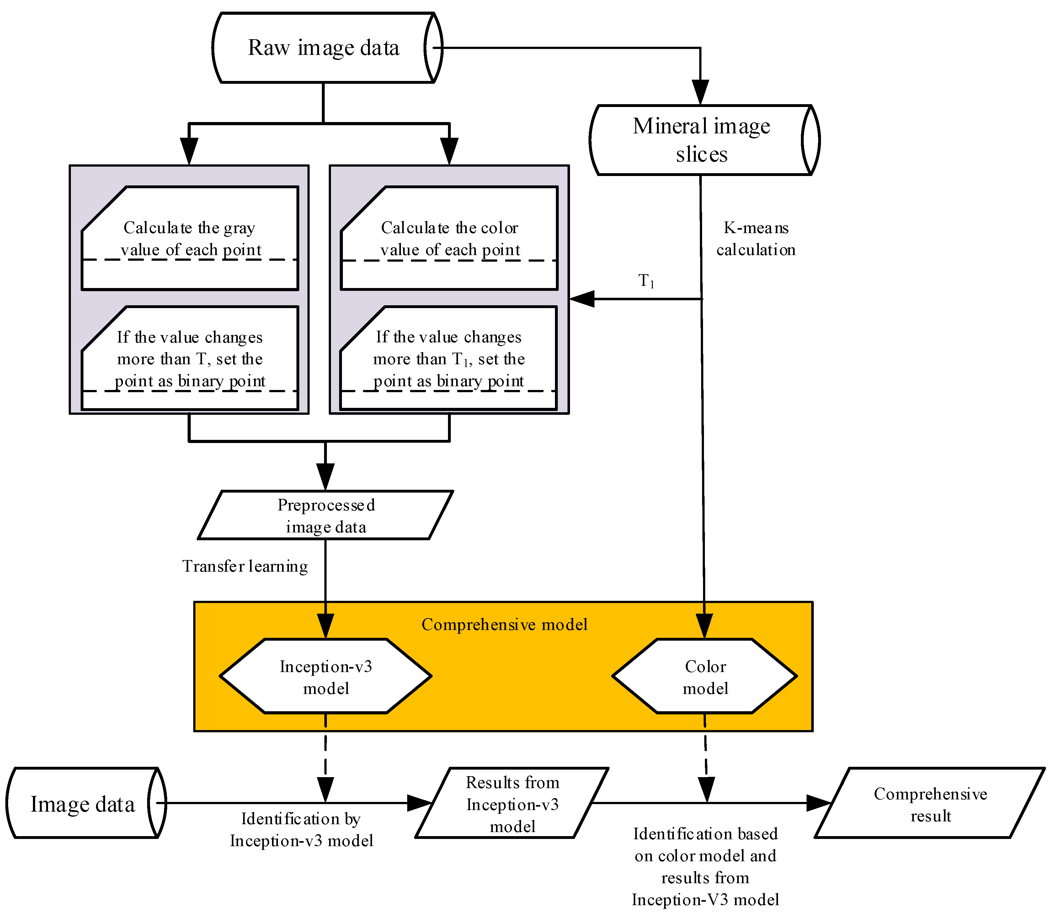
2. Methodology
2.1. Deep Learning Algorithm
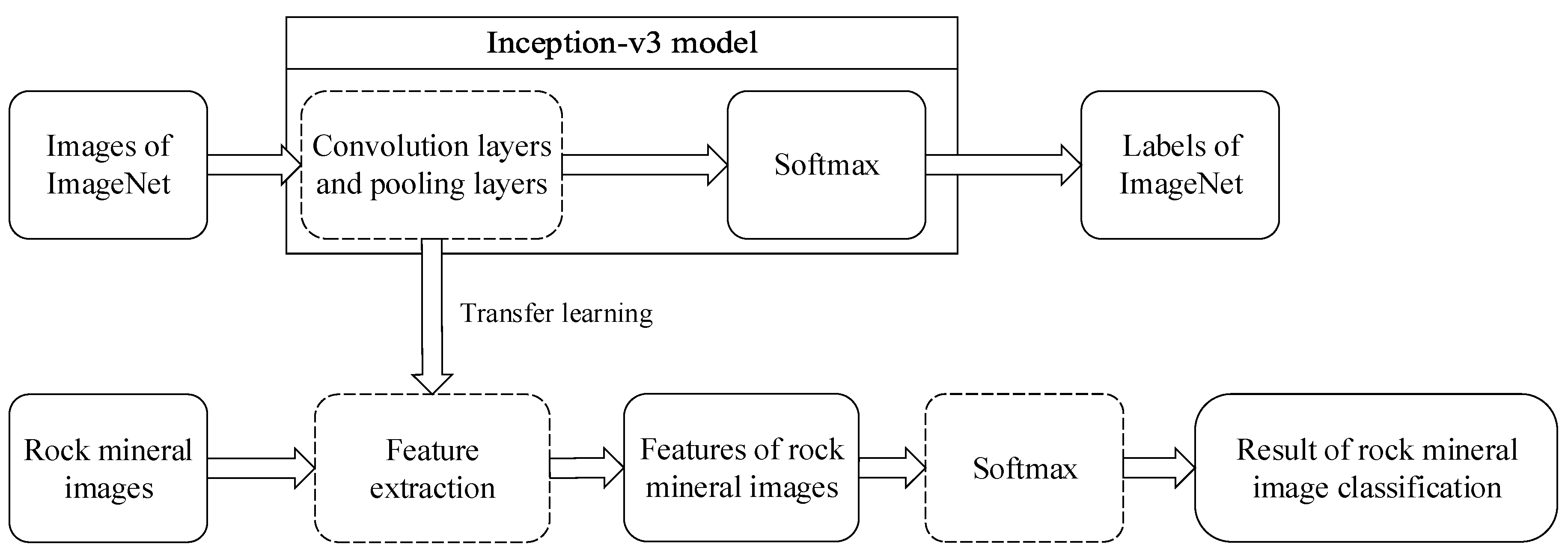
2.2. Transfer Leaning Method
2.3. Clustering Algorithm
2.4. Support Vector Machine
2.5. Random Forest
3. Algorithm Implementation
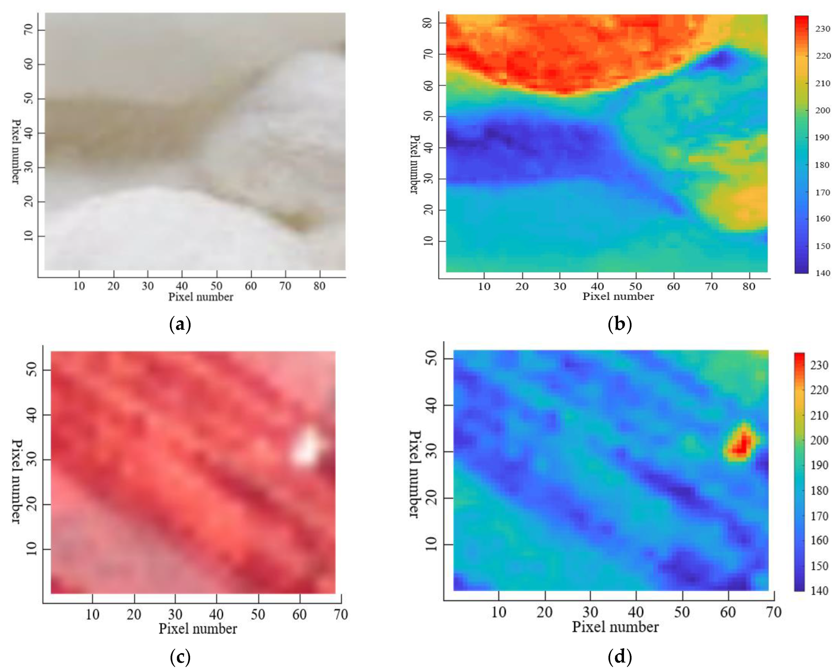
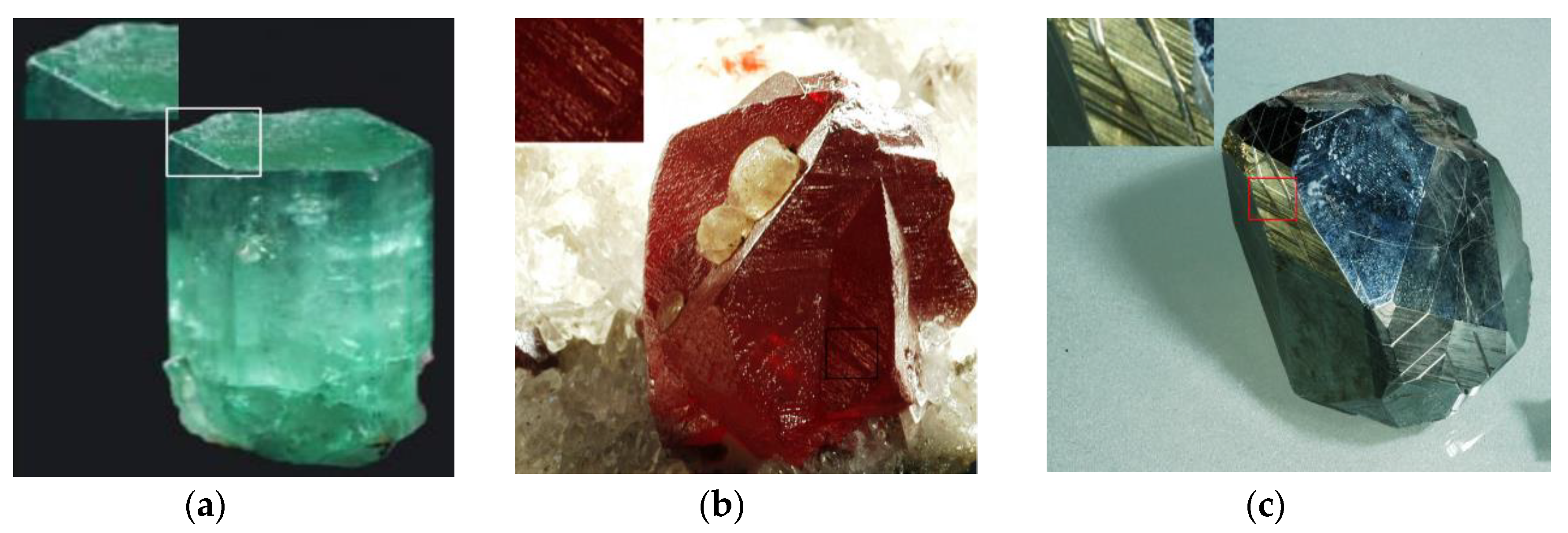
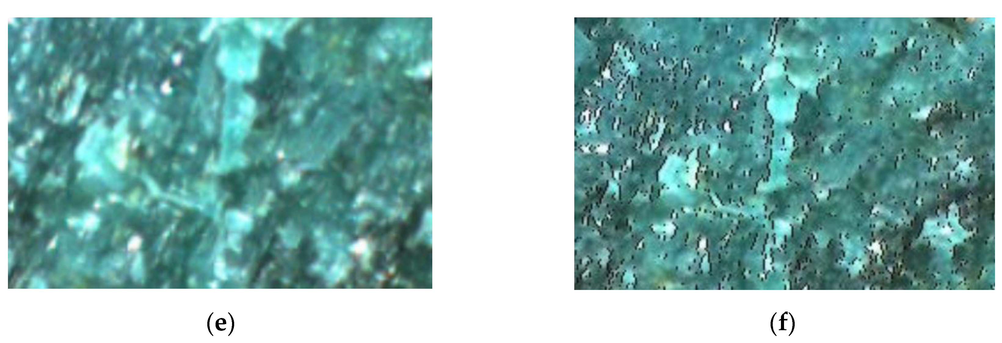
3.1. Mineral Texture Feature Extraction
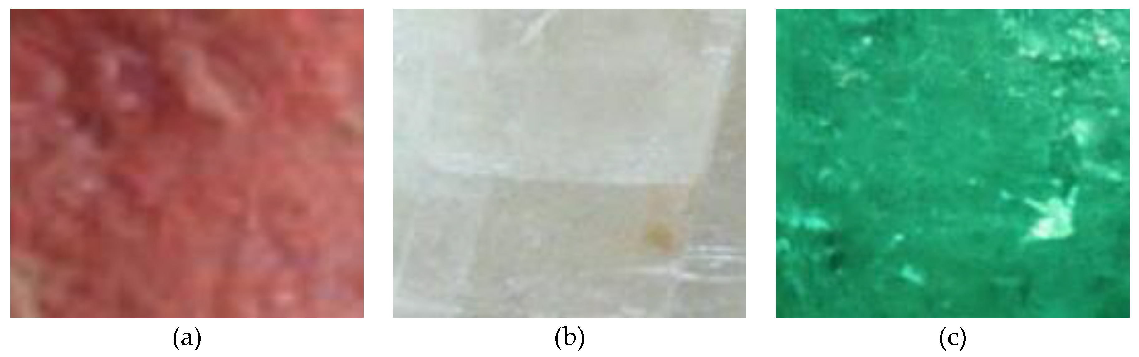
3.2. Color Model of Rock Mineral
4. Experiment and Results
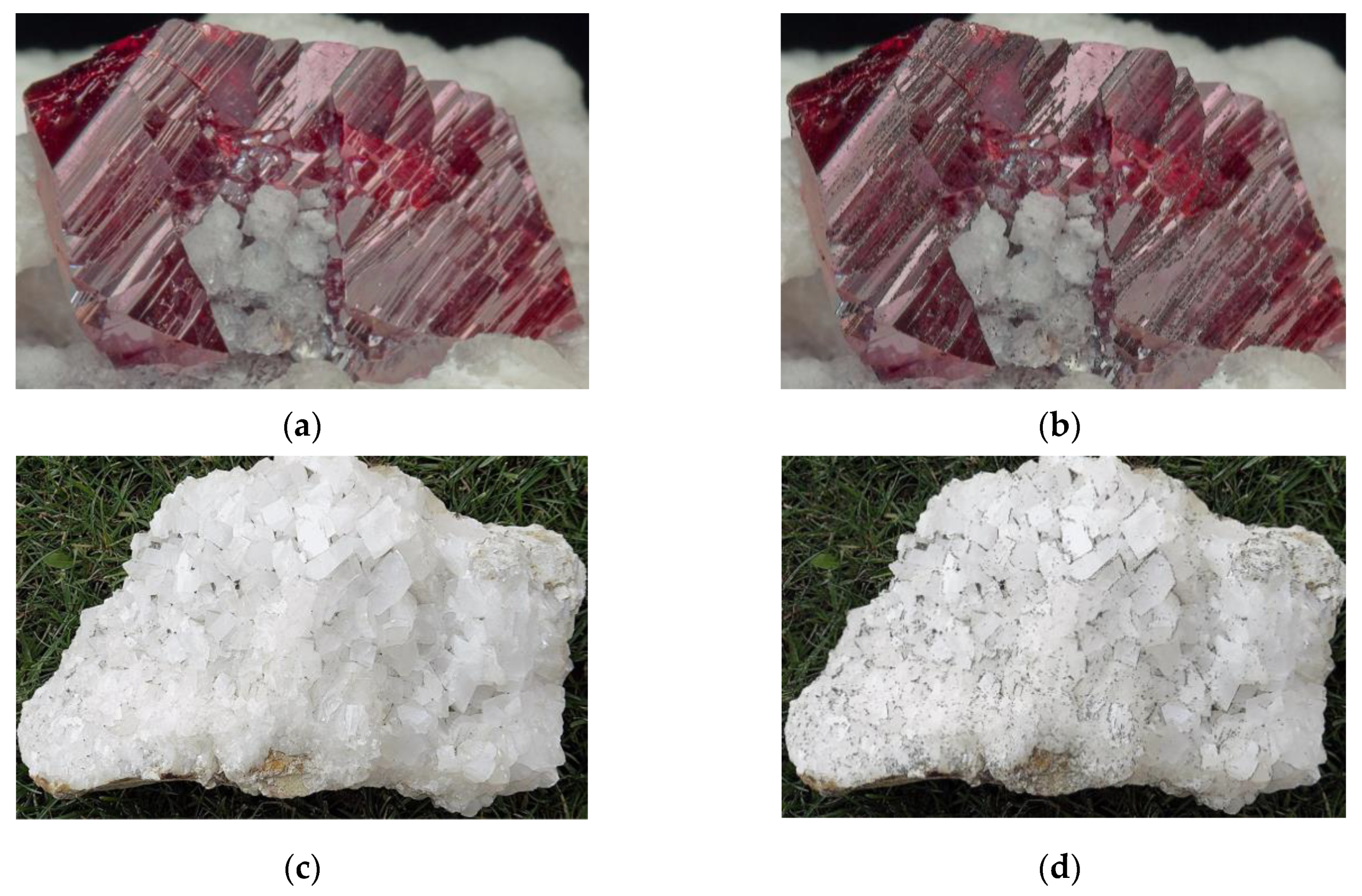
4.1. Image Processing
4.2. Model Establishment
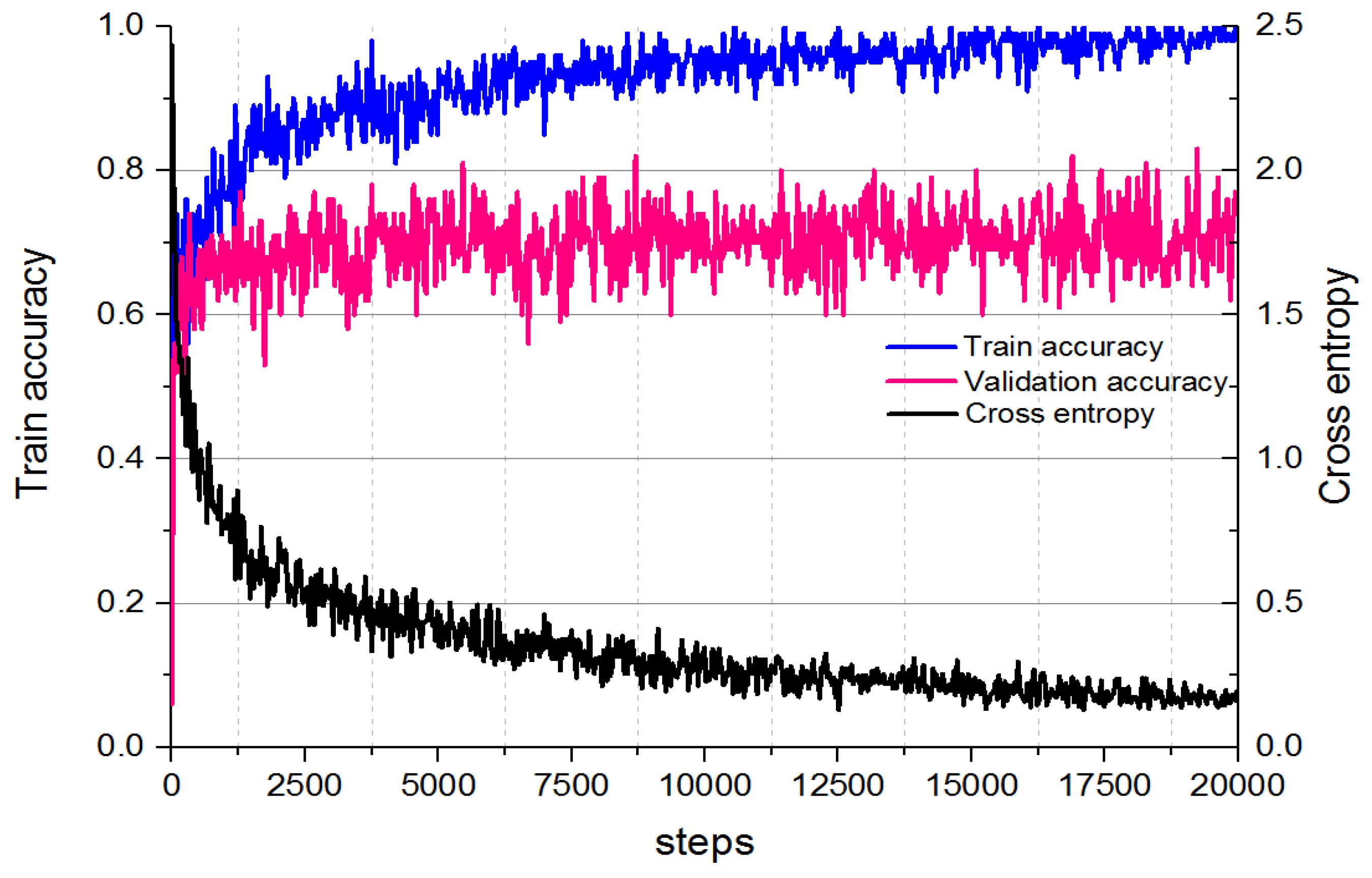
4.2.1. Model Training
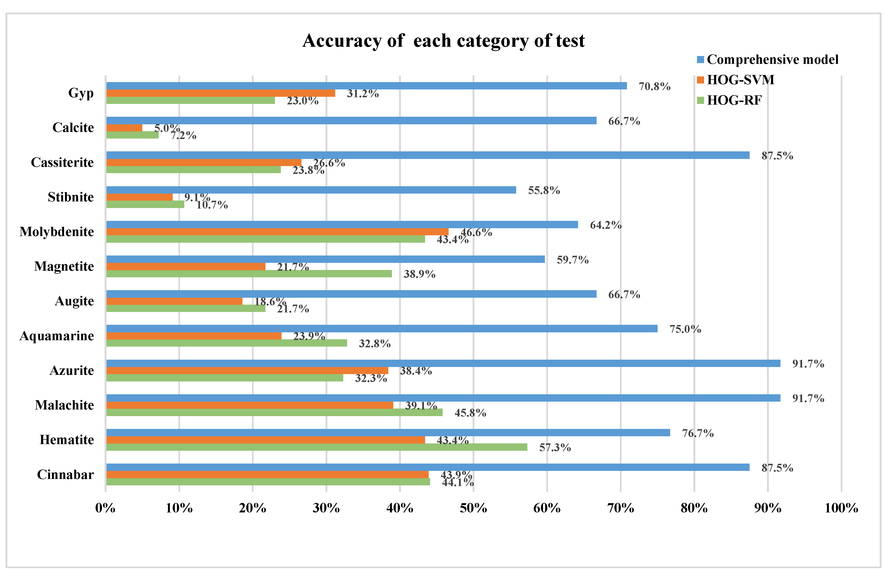
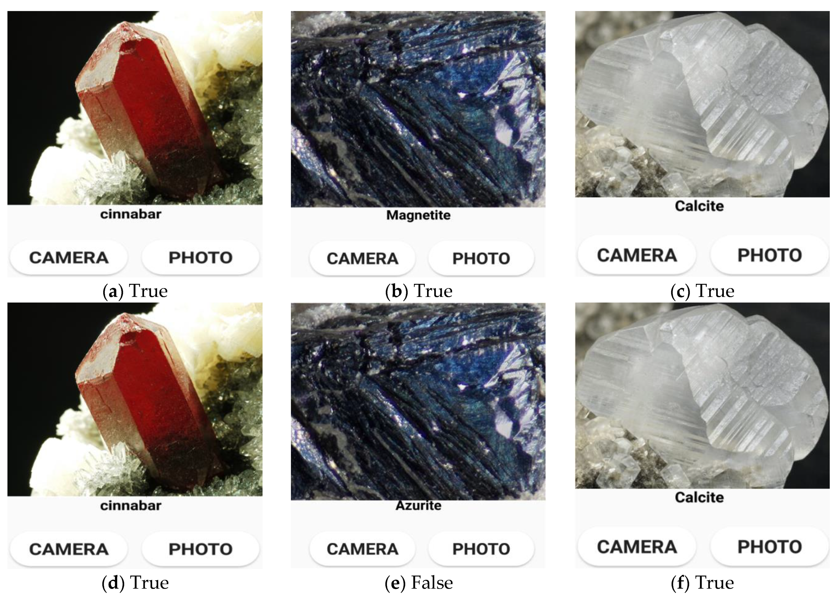
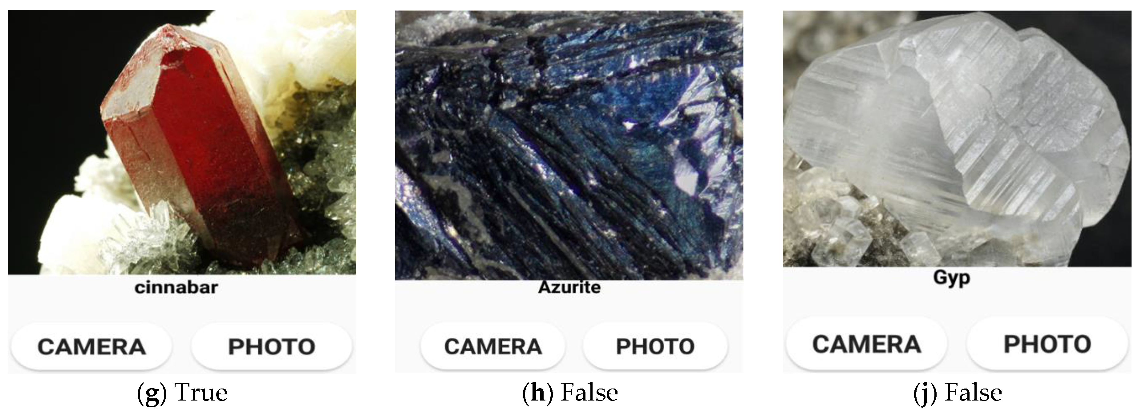
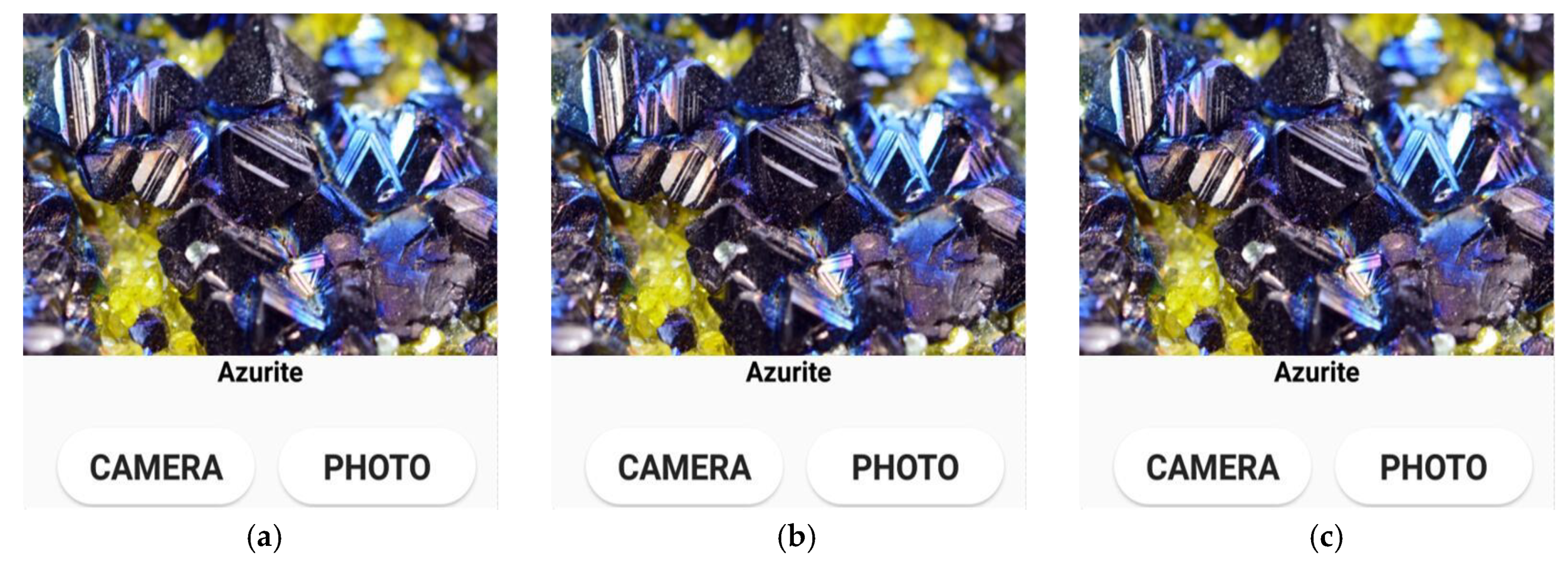
4.2.2. Model Test and Results
5. Conclusions
Author Contributions
Funding
Conflicts of Interest
References
- Yeshi, K.; Wangdi, T.; Qusar, N.; Nettles, J.; Craig, S.R.; Schrempf, M.; Wangchuk, P. Geopharmaceuticals of Himalayan Sowa Rigpa medicine: Ethnopharmacological uses, mineral diversity, chemical identification and current utilization in Bhutan. J. Ethnopharmacol. 2018, 223, 99–112. [Google Scholar] [CrossRef] [PubMed]
- Rustom, L.E.; Poellmann, M.J.; Johnson, A.J.W. Mineralization in micropores of calcium phosphate scaffolds. Acta Biomater. 2019, 83, 435–455. [Google Scholar] [CrossRef] [PubMed]
- Laura, B.; Nina, E.; Mona, W.M.; Udo, Z.; Andò Sergio Merete, M.; Reidar, I.K. Quick, easy, and economic mineralogical studies of flooded chalk for eor experiments using raman spectroscopy. Minerals 2018, 8, 221. [Google Scholar]
- Ramil, A.; López, A.J.; Pozo-Antonio, J.S.; Rivas, T. A computer vision system for identification of granite-forming minerals based on RGB data and artificial neural networks. Measurement 2017, 117, 90–95. [Google Scholar] [CrossRef]
- Sadeghi, B.; Madani, N.; Carranza, E.J.M. Combination of geostatistical simulation and fractal modeling for mineral resource classification. J. Geochem. Explor. 2015, 149, 59–73. [Google Scholar] [CrossRef]
- Li, R.; Albert, N.N.; Yun, M.; Meng, Y.S.; Du, H. Geological and Geochemical Characteristics of the Archean Basement-Hosted Gold Deposit in Pinglidian, Jiaodong Peninsula, Eastern China: Constraints on Auriferous Quartz-Vein Exploration. Minerals 2019, 9, 62. [Google Scholar] [CrossRef]
- Rajendran, S.; Nasir, S. ASTER capability in mapping of mineral resources of arid region: A review on mapping of mineral resources of the Sultanate of Oman. Ore Geol. Rev. 2019, 108, 33–53. [Google Scholar] [CrossRef]
- Shi, B.; Liu, J. Nonlinear metric learning for kNN and SVMs through geometric transformations. Neurocomputing 2018, 318, 18–29. [Google Scholar] [CrossRef] [Green Version]
- Sachindra, D.; Ahmed, K.; Rashid, M.M.; Shahid, S.; Perera, B. Statistical downscaling of precipitation using machine learning techniques. Atmos. Res. 2018, 212, 240–258. [Google Scholar] [CrossRef]
- Vassilev, S.V.; Vassileva, C.G. A new approach for the combined chemical and mineral classification of the inorganic matter in coal. 1. Chemical and mineral classification systems. Fuel 2009, 88, 235–245. [Google Scholar] [CrossRef]
- Vassilev, S.V.; Vassileva, C.G. A new approach for the classification of coal fly ashes based on their origin, composition, properties, and behaviour. Fuel 2007, 86, 1490–1512. [Google Scholar] [CrossRef]
- Zaini, N.; Van Der Meer, F.; Van Der Werff, H. Determination of Carbonate Rock Chemistry Using Laboratory-Based Hyperspectral Imagery. Remote. Sens. 2014, 6, 4149–4172. [Google Scholar] [CrossRef] [Green Version]
- Adep, R.N.; Shetty, A.; Ramesh, H. EXhype: A tool for mineral classification using hyperspectral data. ISPRS J. Photogramm. Remote. Sens. 2017, 124, 106–118. [Google Scholar] [CrossRef]
- Othman, A.A.; Gloaguen, R. Integration of spectral spatial and morphometric data into lithological. J. Asian Earth Sci. 2017, 146, 90–102. [Google Scholar] [CrossRef]
- Li, Y.; Chen, C.; Fang, R.; Yi, L. Accuracy enhancement of high-rate GNSS positions using a complete ensemble empirical mode decomposition-based multiscale multiway PCA. J. Asian Earth Sci. 2018, 169, 67–78. [Google Scholar] [CrossRef]
- Wang, W.; Chen, L. Flotation Bubble Delineation Based on Harris Corner Detection and Local Gray Value Minima. Minerals 2015, 5, 142–163. [Google Scholar] [CrossRef] [Green Version]
- Chen, J.; Chen, Y.; Wang, Q. Synthetic Informational Mineral Resource Prediction: Case Study in Chifeng Region, Inner Mongolia, China. Earth Sci. Front. 2008, 15, 18–26. [Google Scholar] [CrossRef]
- Shardt, Y.A.; Brooks, K. Automated System Identification in Mineral Processing Industries: A Case Study using the Zinc Flotation Cell. IFAC-Papers OnLine 2018, 51, 132–137. [Google Scholar] [CrossRef]
- Ślipek, B.; Młynarczuk, M. Application of pattern recognition methods to automatic identification of microscopic images of rocks registered under different polarization and lighting conditions. Geol. Geophys. Environ. 2013, 39, 373. [Google Scholar] [CrossRef]
- Młynarczuk, M.; Górszczyk, A.; Ślipek, B. The application of pattern recognition in the automatic classification of microscopic rock images. Comput. Geosci. 2013, 60, 126–133. [Google Scholar] [CrossRef]
- Shu, L.; McIsaac, K.; Osinski, G.R.; Francis, R. Unsupervised feature learning for autonomous rock image classification. Comput. Geosci. 2017, 106, 10–17. [Google Scholar] [CrossRef]
- Coates, A.; Ng, A.Y.; Lee, H. An analysis of single-layer networks in unsupervised feature learning. In Proceedings of the 14th International Conference on Artificial Intelligence and Statistics, Fort Lauderdale, FL, USA, 11–13 April 2011; pp. 215–223. [Google Scholar]
- Raina, R.; Battle, A.; Lee, H.; Packer, B.; Ng, A.Y. Self-taught learning: Transfer learning from unlabeled data. In Proceedings of the 24th International Conference on Machine Learning, Corvallis, OR, USA, 20–24 June 2007; pp. 759–766. [Google Scholar]
- Aligholi, S.; Lashkaripour, G.R.; Khajavi, R.; Razmara, M. Automatic mineral identification using color tracking. Pattern Recognit. 2016, 65, 164–174. [Google Scholar] [CrossRef]
- Li, N.; Hao, H.; Gu, Q.; Wang, D.; Hu, X. A transfer learning method for automatic identification of sandstone microscopic images. Comput. Geosci. 2017, 103, 111–121. [Google Scholar] [CrossRef]
- Google Deep Learning. Available online: http://deeplearning.net/tag/google/ (accessed on 21 March 2019).
- Zhang, Y.; Li, M.C.; Han, S. Automatic identification and classification in lithology based on deep learning in rock images. Acta Petrol. Sin. 2018, 34, 333–342. [Google Scholar]
- Kitzig, M.C.; Kepic, A.; Grant, A. Near Real-Time Classification of Iron Ore Lithology by Applying Fuzzy Inference Systems to Petrophysical Downhole Data. Minerals 2018, 8, 276. [Google Scholar] [CrossRef]
- Xiong, Y.; Zuo, R.; Carranza, E.J.M. Mapping mineral prospectivity through big data analytics and a deep learning algorithm. Ore Geol. Rev. 2018, 102, 811–817. [Google Scholar] [CrossRef]
- Zuo, R.; Xiong, Y.; Wang, J.; Carranza, E.J.M. Deep learning and its application in geochemical mapping. Earth-Sci. Rev. 2019, 192, 1–14. [Google Scholar] [CrossRef]
- Iglesias, J.C.; Álvarez; Santos, R.B.M.; Paciornik, S. Deep learning discrimination of quartz and resin in optical microscopy images of minerals. Miner. Eng. 2019, 138, 79–85. [Google Scholar] [CrossRef]
- Hinton, G.E.; Salakhutdinov, R.R. Reducing the Dimensionality of Data with Neural Networks. Science 2006, 313, 504–507. [Google Scholar] [CrossRef] [Green Version]
- Hinton, G.; Mohamed, A.-R.; Jaitly, N.; Vanhoucke, V.; Kingsbury, B.; Deng, L.; Yu, D.; Dahl, G.; Senior, A.; Nguyen, P.; et al. Deep Neural Networks for Acoustic Modeling in Speech Recognition: The Shared Views of Four Research Groups. IEEE Signal Process. Mag. 2012, 29, 82–97. [Google Scholar] [CrossRef]
- Gong, M.; Yang, H.; Zhang, P. Feature learning and change feature classification based on deep learning for ternary change detection in SAR images. ISPRS J. Photogramm. Remote Sens. 2017, 129, 212–225. [Google Scholar] [CrossRef]
- Pham, C.C.; Jeon, J.W. Robust object proposals re-ranking for object detection in autonomous driving using convolutional neural networks. Signal Process. Image Commun. 2017, 53, 110–122. [Google Scholar] [CrossRef]
- Esteva, A.; Kuprel, B.; Novoa, R.A.; Ko, J.; Swetter, S.M.; Blau, H.M.; Thrun, S. Dermatologist-level classification of skin cancer with deep neural networks. Nature 2017, 542, 115–118. [Google Scholar] [CrossRef]
- Szegedy, C.; Vanhoucke, V.; Ioffe, S.; Shlens, J.; Wojna, Z. Rethinking the Inception Architecture for Computer Vision. In Proceedings of the 2016 IEEE Conference on Computer Vision and Pattern Recognition (CVPR), Las Vegas, NV, USA, 26 June–1 July 2016; pp. 2818–2826. [Google Scholar]
- Qureshi, A.S.; Khan, A.; Zameer, A.; Usman, A. Wind power prediction using deep neural network based meta regression and transfer learning. Appl. Soft Comput. 2017, 58, 742–755. [Google Scholar] [CrossRef]
- Xu, G.; Zhu, X.; Fu, D.; Dong, J.; Xiao, X. Automatic land cover classification of geo-tagged field photos by deep learning. Environ. Model. Softw. 2017, 91, 127–134. [Google Scholar] [CrossRef] [Green Version]
- Xu, B.; Shen, S.; Shen, F.; Zhao, J. Locally linear SVMs based on boundary anchor points encoding. Neural Netw. 2019, 117, 274–284. [Google Scholar] [CrossRef]
- Pellant, C. Rocks and Minerals—Smithsonian Handbook; DK Publisher: New York, NY, USA, 2002. [Google Scholar]
- The Geological Museum of China. Available online: http://www.gmc.org.cn (accessed on 28 March 2019).
- International Telecommunication Union. Available online: https://www.itu.int/rec/R-REC-BT.601-7-201103-I/en (accessed on 12 March 2019).


| Minerals | Color | Streak | Transparency | Aggregate Shape | Luster |
|---|---|---|---|---|---|
| Cinnabar | Red | Red | Translucent | Granule, massive form | Adamantine luster |
| Hematite | Red | Cherry red | Opaque | Multi-form | From metallic luster to soil state luster |
| Calcite | Colorless or white | White | Translucent | Granule, massive form, threadiness, stalactitic form, soil state | Glassy luster |
| Malachite | Green | Pale green | From translucent to opaque | Emulsions, massive, incrusting, concretion forms or threadiness | Waxy luster, glassy luster, soil state luster |
| Azurite | Navy blue | Pale blue | Opaque | Granule, stalactitic, incrusting, soil state | Glassy luster |
| Aquamarine | Determine by its component | White | Transparent | Cluster form | Glassy luster |
| Augite | Black | Pale green, black | Opaque | Granule, radial pattern, massive | Glassy luster |
| Magnetite | Black | Black | Opaque | Granule, massive form | Metallic luster |
| Molybdenite | Gray | Light gray | Opaque | Clintheriform, scaly form or lobate form | Metallic luster |
| Stibnite | Gray | Dark gray | Opaque | Massive, granule or radial pattern | Strong metallic luster |
| Cassiterite | Crineus, yellow, black | White, pale brown | From opaque to transparent | Irregular granule | Adamantine luster, sub adamantine luster |
| Gyp | White, colorless | White | Transparent, translucent | Clintheriform, massive, threadiness | Glassy luster, nacreous luster |
| Rock Minerals | Number | Rock Minerals | Number |
|---|---|---|---|
| Cinnabar | 327 | Hematite | 324 |
| Aquamarine | 380 | Calcite | 451 |
| Molybdenite | 316 | Stibnite | 423 |
| Malachite | 335 | Azurite | 323 |
| Cassiterite | 378 | Augite | 171 |
| Magnetite | 335 | Gyp | 415 |
| Rock Minerals | Colors (R, G, B) | ||
|---|---|---|---|
| Color1 | Color2 | Color3 | |
| Cinnabar | (142,79,69) | (105,36,31) | (184,107,102) |
| Hematite | (168,96,80) | (127,157,138) | - |
| Molybdenite | (121,125,126) | (93,96,98) | - |
| Calcite | (193,199,193) | (175,177,167) | - |
| Cassiterite | (44,47,53) | - | - |
| Magnetite | (36,33,31) | - | - |
| Malachite | (88,168,129) | (67,144,104) | (50,108,75) |
| Azurite | (0,19,151) | (44,77,201) | - |
| Aquamarine | (0,95,56) | (35,159,112) | - |
| Augite | (82,80,82) | (122,120,124) | - |
| Stibnite | (92,104,115) | - | - |
| Gyp | (161,161,163) | (230,220,192) | - |
| Models | Validation Accuracy | Test Accuracy | |
|---|---|---|---|
| Top-1 | Top-3 | ||
| Model based on raw images | 73.1% | 64.1% | 96.0% |
| Model based on texture extraction images | 77.4% | 67.5% | 98.3% |
| Comprehensive model | 77.4% | 74.2% | 99.0% |
| SVM-HOG | 33.6% 30.4% | ||
| RF-HOG | |||
| Models | Precision Rate | Recall Rate | F1-measure Value |
|---|---|---|---|
| Comprehensive model | 74.2% | 77.5% | 0.758 |
| SVM-HOG | 33.6% | 28.5% | 0.308 |
| RF-HOG | 30.4% | 31.2% | 0.308 |
© 2019 by the authors. Licensee MDPI, Basel, Switzerland. This article is an open access article distributed under the terms and conditions of the Creative Commons Attribution (CC BY) license (http://creativecommons.org/licenses/by/4.0/).
Share and Cite
Liu, C.; Li, M.; Zhang, Y.; Han, S.; Zhu, Y. An Enhanced Rock Mineral Recognition Method Integrating a Deep Learning Model and Clustering Algorithm. Minerals 2019, 9, 516. https://doi.org/10.3390/min9090516
Liu C, Li M, Zhang Y, Han S, Zhu Y. An Enhanced Rock Mineral Recognition Method Integrating a Deep Learning Model and Clustering Algorithm. Minerals. 2019; 9(9):516. https://doi.org/10.3390/min9090516
Chicago/Turabian StyleLiu, Chengzhao, Mingchao Li, Ye Zhang, Shuai Han, and Yueqin Zhu. 2019. "An Enhanced Rock Mineral Recognition Method Integrating a Deep Learning Model and Clustering Algorithm" Minerals 9, no. 9: 516. https://doi.org/10.3390/min9090516
APA StyleLiu, C., Li, M., Zhang, Y., Han, S., & Zhu, Y. (2019). An Enhanced Rock Mineral Recognition Method Integrating a Deep Learning Model and Clustering Algorithm. Minerals, 9(9), 516. https://doi.org/10.3390/min9090516