Acquisition and Processing of Wider Bandwidth Seismic Data in Crystalline Crust: Progress with the Metal Earth Project

 ,
,
Abstract
1. Introduction
2. Seismic Data Acquisition
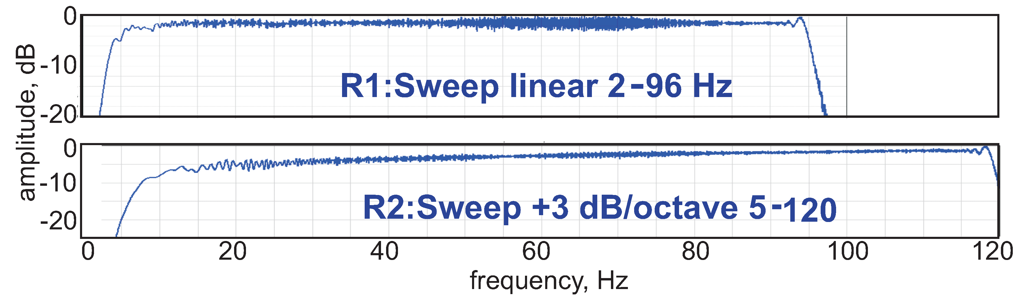
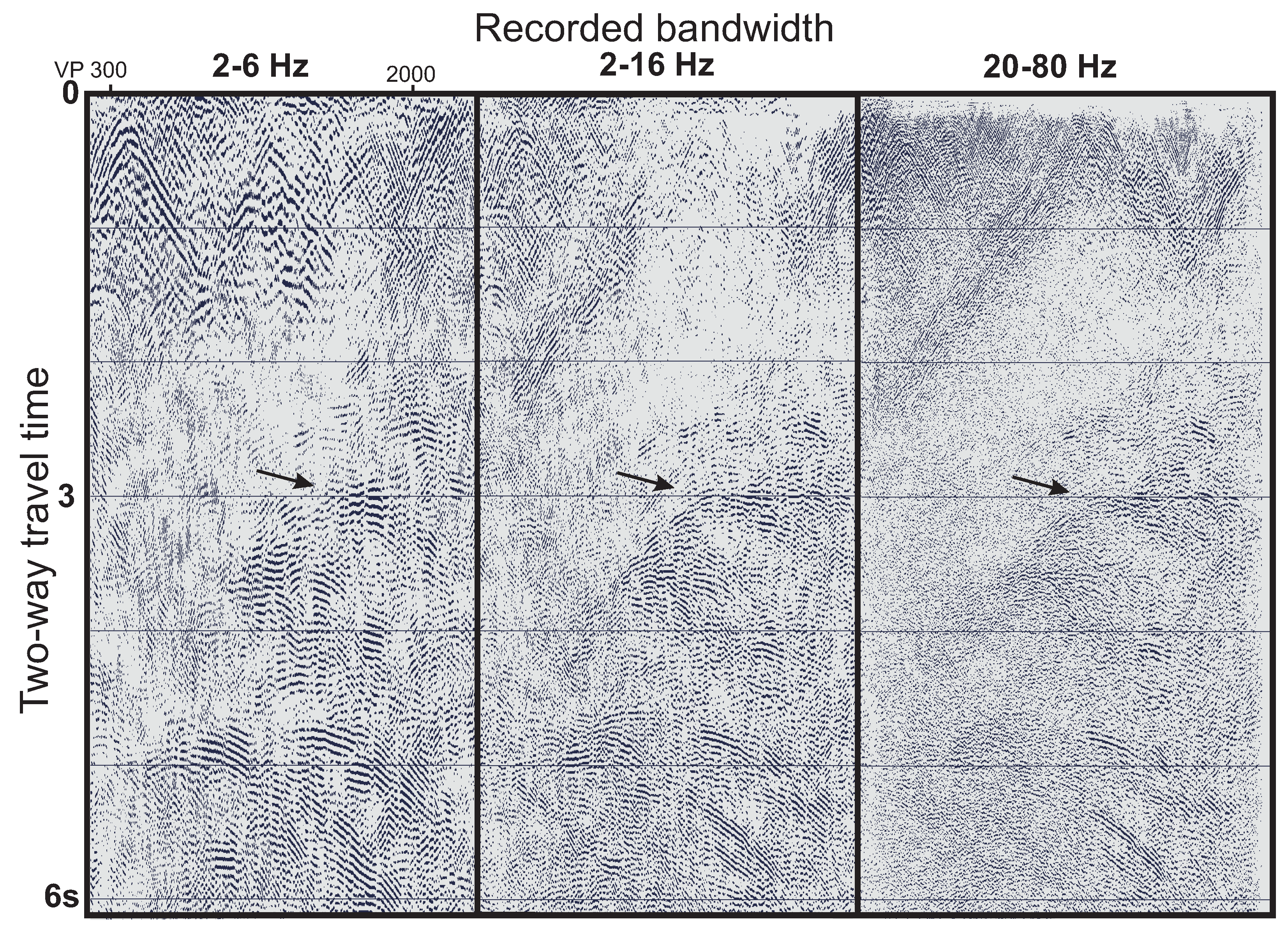
2.1. Improved Bandwidth
2.2. Source Arrays
2.3. Toward Using Full Waveforms
3. Seismic Data Processing
3.1. Geometry Check
3.2. Amplitude and Phase Corrections
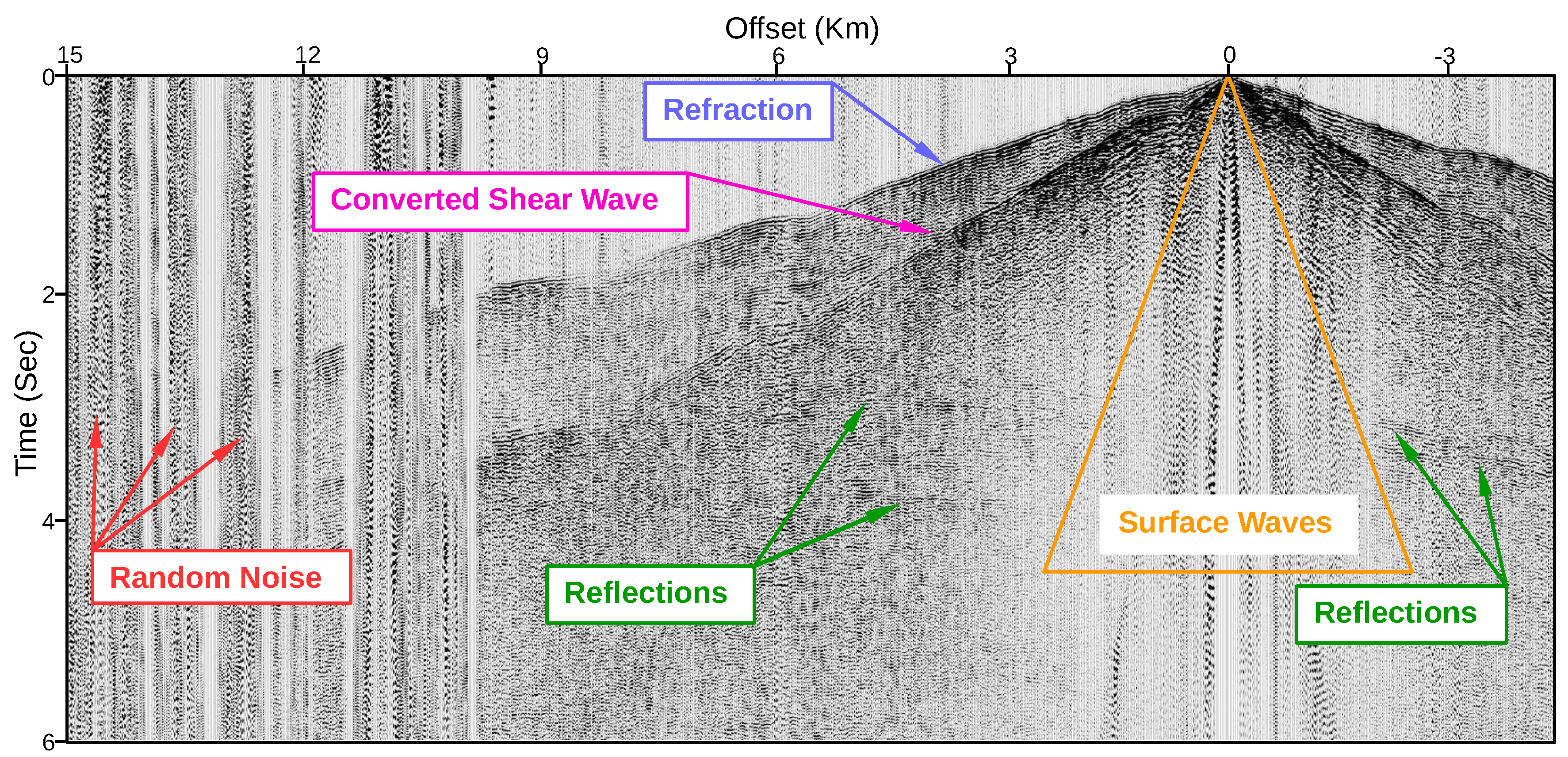
3.3. Random and Coherent Noise Attenuation
3.4. Surface Consistent Deconvolution
3.5. Near-Surface Refraction Analysis
3.6. Velocity Analysis and Statics Correction
3.7. Post-Stack Kirchhoff Migration
3.8. Pre-Stack Kirchhoff Migration
3.9. Post-Migration Processing
4. Discussion
5. Conclusions
Author Contributions
Funding
Acknowledgments
Conflicts of Interest
References
- Eaton, D.W.; Milkereit, B.; Salisbury, M.H. Hardrock seismic exploration. Soc. Explor. Geophys. 2003, 10, 1–269. [Google Scholar]
- Ten Kroode, F.; Bergler, S.; Corsten, C.; de Maag, J.W.; Strijbos, F.; Tijhof, H. Broadband seismic data—The importance of low frequencies. Geophysics 2013, 78, WA3–WA14. [Google Scholar] [CrossRef]
- Calvert, A.J.; Ludden, J.N. Archean continental assembly in the southeastern Superior Province of Canada. Tectonics 1999, 18, 412–429. [Google Scholar] [CrossRef]
- Ludden, J.; Hynes, A. The Lithoprobe Abitibi-Grenville transect: Two billion years of crust formation and recycling in the Precambrian Shield of Canada. Can. J. Earth Sci. 2000, 37, 459–476. [Google Scholar] [CrossRef]
- White, D.J.; Musacchio, G.; Helmstaedt, H.H.; Harrap, R.M.; Thurston, P.C.; Van der Velden, A.; Hall, K. Images of a lower-crustal oceanic slab: Direct evidence for tectonic accretion in the Archean western Superior province. Geology 2003, 31, 997–1000. [Google Scholar] [CrossRef]
- Snyder, D.B.; Bleeker, W.; Reed, L.E.; Ayer, J.A.; Houle, M.G.; Bateman, R. Tectonic and metallogenic implications of regional seismic profiles in the timmins mining camp. Econ. Geol. 2008, 103, 1135–1150. [Google Scholar] [CrossRef]
- Boore, D.M.; Atkinson, G.M. Stochastic prediction of ground motion and spectral response parameters at hard-rock sites in eastern North America. Bull. Seismol. Soc. Am. 1987, 77, 440–467. [Google Scholar]
- Malinowski, M. Deep reflection seismic imaging in SE Poland using extended correlation method applied to PolandSPAN™ data. Tectonophysics 2016, 689, 107–114. [Google Scholar] [CrossRef]
- Snyder, D.B.; Cary, P.; Salisbury, M. 2D-3C high-resolution seismic data from the Abitibi Greenstone Belt, Canada. Tectonophysics 2009, 472, 226–237. [Google Scholar] [CrossRef]
- Bellefleur, G.; Schetselaar, E.; White, D.; Miah, K.; Dueck, P. 3D seismic imaging of the Lalor volcanogenic massive sulphide deposit, Manitoba, Canada. Geophys. Prospect. 2015, 63, 813–832. [Google Scholar] [CrossRef]
- Pratt, R.G.; Shin, C.; Hicks, G.J. Gauss-Newton and full Newton methods in frequency-space seismic waveform inversion. Geophys. J. Int. 1998, 133, 341–362. [Google Scholar] [CrossRef]
- Virieux, J.; Operto, S. An overview of full-waveform inversion in exploration geophysics. Geophysics 2009, 74, WCC1–WCC26. [Google Scholar] [CrossRef]
- Bunks, C.; Saleck, F.M.; Zaleski, S.; Chavent, G. Multiscale seismic waveform inversion. Geophysics 1995, 60, 1457–1473. [Google Scholar] [CrossRef]
- Smithyman, B.R.; Clowes, R.M. Waveform tomography in 2.5D: Parameterization for crooked-line acquisition geometry. J. Geophys. Res. Solid Earth 2013, 118, 2119–2137. [Google Scholar] [CrossRef]
- Kamei, R.; Miyoshi, T.; Pratt, R.G.; Takanashi, M.; Masaya, S. Application of waveform tomography to a crooked-line 2D land seismic data set. Geophysics 2015, 80, B115–B129. [Google Scholar] [CrossRef]
- Nedimovic, M.R.; West, G.F. Crooked-line 2D seismic reflection imaging in crystalline terrains: Part 1, data processing. Geophysics 2003, 68, 274–285. [Google Scholar] [CrossRef]
- Cary, P.W.; Lorentz, G.A. Four-component surface-consistent deconvolution. Geophysics 1993, 58, 383–392. [Google Scholar] [CrossRef]
- Taner, M.T.; Koehler, F. Surface consistent corrections. Geophysics 2002, 46, 17–22. [Google Scholar] [CrossRef]
- Yilmaz, O. Seismic Data Analysis: Processing, Inversion, and Interpretation of Seismic Data; Society of Exploration Geophysicists: Tulsa, OK, USA, 2014. [Google Scholar]
- Zhang, J.; Toksöz, M.N. Nonlinear refraction traveltime tomography. Geophysics 1998, 63, 1726–1737. [Google Scholar] [CrossRef]
- Gray, S.H.; Etgen, J.; Dellinger, J.; Whitmore, D. Seismic migration problems and solutions. Geophysics 2001, 66, 1622–1640. [Google Scholar] [CrossRef]
- Postlethwaite, B.; Bostock, M.G.; Christensen, N.I.; Snyder, D.B. Seismic velocities and composition of the Canadian crust. Tectonophysics 2014, 633, 256–267. [Google Scholar] [CrossRef]


| Parameter | Regional (R1) Mode | High-Resolution (R2) Mode | Full-Waveform (R3) Mode |
|---|---|---|---|
| Record length | 12 or 16 s | 12 s | 12 s |
| Sample rate | 2 ms | 2 ms | 2 ms |
| Spread size | 15 km–0–15 km | All live (10–20 km) | All live (30–80 km) |
| Roll on/off | Yes | Yes | Yes |
| Source interval | 50 m (4 sweeps); 12.5 m (1 sweep) | 25 m (4 sweeps); 6.25 m (1 sweep) | As in R1 |
| Receiver interval | 25 m | 12.5 m | 25 m |
| Vibrator sweep | 28 s, 2–96 Hz linear; 4 vibs; | 28 s, 5–120 Hz + 3db/octave; 3 vibs; | As in R1 |
| Transect Name | Length, km | Acquisition Modes | Comment |
|---|---|---|---|
| Chibougamau | 129.85 | R1, R2 × 2 | No vibrator move-up |
| Malartic | 84.775 | R1, R3 | Major gap near Malartic Mine/Town |
| Rouyn-Noranda | 84.775 | R1, R3 | Crooked line; coincident with Lithoprobe AG-21 |
| Larder Lake | 49 | R1, R2, R3 | coincident with Lithoprobe AG-23 |
| Cobalt | 46.375 | R1, R2 | |
| Matheson | 53.95 | R1, R2 | R1, R2 offset |
| Swayze | 89.35, 11.8 | R1, R2 × 3 | |
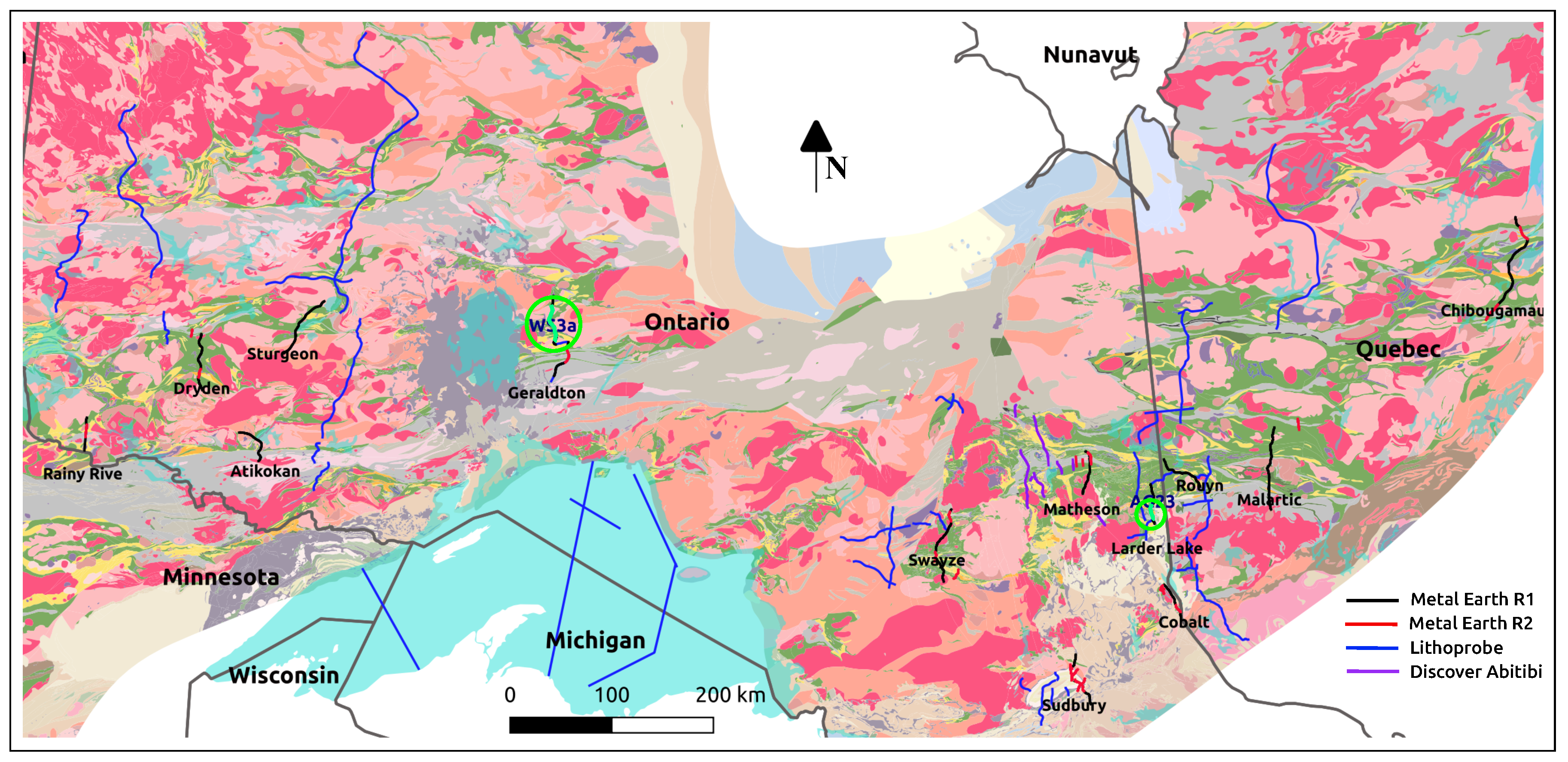
| Geraldton | 60.2125 | R1 × 2, R2 | Coincident with Lithoprobe WS-3a |
| Sturgeon Lake | 73.475 | R1 | |
| Atikokan | 54.1 | R1 | Crooked line |
| Dryden | 74.4 | R1, R2 × 2 | |
| Rainy River | 33.15 | R1, R2 | |
| Sudbury | 39, 17, 16, 10 | R1 × 3, R2 × 2, R3 | Grid of lines |
| Processing Step | Parameters Used | Comment |
|---|---|---|
| Trace Kills and Reversals | ||
| Min Phase Conversion | ||
| Ensemble Balance, Amplitude Recovery | Time power correction + 1.5 | |
| Surface Conistent Scaling | ||
| Linear and Erratic Noise Attenuation | ||
| Surface-Consistent Deconvolution | Operator: 160 ms Prewhitening: 0.1 % | Design window: 171–10,000 ms at 38 m offset 3347–10,000 ms at 15,000 m offset |
| Anomalous Frequency Suppression | Desired output band: 5–100 Hz Signal band: 15–50 Hz | |
| Refraction Statics | Datum: 500 m Replacement Velocity: 5600 m/s | Tomography |
| Linear and Erratic Noise Attenuation | ||
| TE Mean window | Design window: 171–10,000 ms at 38 m offset 3347–10,000 ms at 15,000 m offset | |
| Velocity Analysis | Every 1.0 km | |
| Surface Consistent Residual Statics | Max shift 64 ms Window: 2000–9000 ms | |
| Velocity Analysis2 | Every 500 m | |
| Surface Consistent Residual Statics | Max shift 48 ms Window: 1000–9000 ms | |
| Post-Stack Time migration | ||
| Velocity Analysis | ||
| Normal Move-out & Mute | ||
| CDP stack | ||
| Time Migration | Kirchhoff Summation | Migration Angle: 65 degrees Max Aperture: 15,000 m |
| Pre-Stack Time migration (PSTM) | ||
| Velocity Analysis (PSTM) | Kirchhoff Summation | VP-CDP Distance: ≤500 m |
| Trace Equalization window | Rolling Window: 1000 ms Overlap 50% | |
| Pre Stack Time Migration (PSTM) | Kirchhoff Summation | Migration Angle: 65 degrees Max Aperture: 10,000 m |
| Front-End Muting | 3/93 1067/758 3554/1871 8028/2778 (m/ms) | |
| CDP Stack | ||
| Random Noise Attenuation | ||
| TraceEqualization window | Rolling Window: 1000 ms Overlap 50% |
| Parameter | Metal Earth (R1) | Lithoprobe WS 3a | Lithoprobe AG 23 |
|---|---|---|---|
| Year | autumn, 2017 | March, 2000 | November, 1990 |
| Contractor | SAExploration | Kinetex | J.R.S. Exploration |
| Record length | 12 or 16 s | 18 s | 18 s |
| Sample rate | 2 ms | 4 ms | 4 ms |
| Spread size | 15 km–0–15 km | 12 km–0–12 km | 8.1 km–0–8.1 km |
| Vibrator; length | I/O AHV-IV 364; 10 m | I/O AHV-IV 360; 10 m | Mertz-18; 11 m |
| Source interval | 12.5 m (1 sweep) 50 m (4 sweeps 0 or 1 m move up) | 100 m (8 sweeps) 7.14 m move up | 100 m (8 sweeps) 7.14 m move up |
| Vibrator sweep | 28 s, 2–96 Hz linear; 4 vibs; | 28 s, 10–84 Hz linear; 4 vibs; | 14 s, 10–56 Hz linear; 4 vibes |
| Receiver interval | 25 m | 25 m | 50 m |
| Geophones | 5 Hz; Single | 10 Hz; 9 over 25 m | 14 Hz; 9 over 50 m |
© 2019 by the authors. Licensee MDPI, Basel, Switzerland. This article is an open access article distributed under the terms and conditions of the Creative Commons Attribution (CC BY) license (http://creativecommons.org/licenses/by/4.0/).
Share and Cite
Naghizadeh, M.; Snyder, D.; Cheraghi, S.; Foster, S.; Cilensek, S.; Floreani, E.; Mackie, J. Acquisition and Processing of Wider Bandwidth Seismic Data in Crystalline Crust: Progress with the Metal Earth Project. Minerals 2019, 9, 145. https://doi.org/10.3390/min9030145
Naghizadeh M, Snyder D, Cheraghi S, Foster S, Cilensek S, Floreani E, Mackie J. Acquisition and Processing of Wider Bandwidth Seismic Data in Crystalline Crust: Progress with the Metal Earth Project. Minerals. 2019; 9(3):145. https://doi.org/10.3390/min9030145
Chicago/Turabian StyleNaghizadeh, Mostafa, David Snyder, Saeid Cheraghi, Steven Foster, Samo Cilensek, Elvis Floreani, and Jeff Mackie. 2019. "Acquisition and Processing of Wider Bandwidth Seismic Data in Crystalline Crust: Progress with the Metal Earth Project" Minerals 9, no. 3: 145. https://doi.org/10.3390/min9030145
APA StyleNaghizadeh, M., Snyder, D., Cheraghi, S., Foster, S., Cilensek, S., Floreani, E., & Mackie, J. (2019). Acquisition and Processing of Wider Bandwidth Seismic Data in Crystalline Crust: Progress with the Metal Earth Project. Minerals, 9(3), 145. https://doi.org/10.3390/min9030145