Quantum Mechanical Modeling of the Vibrational Spectra of Minerals with a Focus on Clays

Abstract

We present an overview of how to use quantum mechanical calculations to predict vibrational frequencies of molecules and materials such as clays and silicates. Other methods of estimating vibrational frequencies are mentioned, such as classical molecular dynamics simulations; references are given for additional information on these approaches. Herein, we discuss basic vibrational theory, calculating Raman and infrared intensities, steps for creating realistic models, and applications to spectroscopy, thermodynamics, and isotopic fractionation. There are a wide variety of programs and methods that can be employed to model vibrational spectra, but this work focuses on hybrid density functional theory (DFT) approaches. Many of the principles are the same when used in other programs and DFT methods, so a novice can benefit from simple examples that illustrate key points to consider when modeling vibrational spectra. Other methods and programs are listed to give the beginner a starting point for exploring and choosing which approach will be best for a given problem. The modeler should also be aware of the numerous analytical methods available for obtaining information on vibrations of atoms in molecules and materials. In addition to traditional infrared and Raman spectroscopy, sum-frequency generation (SFG) and inelastic neutron scattering (INS) are also excellent techniques for obtaining vibrational frequency information in certain circumstances.

1. Introduction

Vibrational spectroscopy—infrared (IR), Raman, and sum-frequency generation (SFG)—are excellent techniques for probing the nature of bonding in fine-grained, poorly crystalline, and highly disordered materials. Clays often fall into this category, as do myriad materials associated with clays such as allophane, imogolite, ferrihydrite, organic matter, and any form of adsorbed surface complex. Consequently, vibrational spectroscopy has been commonly applied to study industrial processes, soils, geochemistry, and health-related chemistry.

In addition to using vibrational spectra to identify phases and determine structures in molecules and materials, vibrational frequencies are also useful in predicting thermodynamics via the vibrational partition function (see McQuarrie and Simon for an excellent chapter on the subject) [1] and isotopic fractionations [2,3]. Thus, the ability to predict vibrational frequencies via computational chemistry has a huge number of applications. When one is confident in the accuracy of the computational technique, it is also possible to follow reaction pathways and use the vibrational partition functions of the reactants, products and transition state to predict the activation energies and rate constants of reactions [4]. Because the computational chemistry approach contains all the atomic-level details about a system of interest, these methods can be used to help interpret experimental data and make predictions about systems or conditions where experiments are not currently feasible.

Before delving into the details of performing vibrational frequency calculations and applying these methods to geochemical problems, we must discuss an important example of the role of vibrational frequencies in our planet and society. The issue of human-induced climate change or global warming is so widely discussed in the media that almost everyone has heard of this issue and most have come to some conclusion about it. However, we doubt that the vast majority of non-scientists realize that the fundamentals of this problem come down to molecular physics. What makes a compound in our atmosphere a “greenhouse gas” is the overlap of its vibrational frequencies with the infrared region (i.e., heat) of the electromagnetic spectrum. This lack of knowledge is obvious when someone states that they do not see how a trace gas such as carbon dioxide (CO₂) can influence the temperature of the planet. The reasoning is that CO₂ is “only” present at approximately 400 ppm (0.04%), whereas N₂ and O₂ make up approximately 79% and 20% of the atmosphere, respectively. This line of thinking does not recognize the fact that N₂ and O₂ absorb no infrared radiation because their strong triple N≡N and double O=O bonds vibrate at much higher frequencies than the infrared part of the spectrum. (This is why the sky is blue, due to scattering of visible radiation by N₂.) CO₂ and other greenhouse gases, on the other hand, have bonds that vibrate at frequencies that absorb IR (heat) and affect the temperature of the Earth’s atmosphere.

No serious person could argue that these principles of molecular physics do not exist, because they are readily measurable in a laboratory. Consequently, the most basic argument for hypothesizing a link between atmospheric CO₂ concentrations and the temperature of the atmosphere (aka “global warming”) comes down to Beer’s Law. This well-known principle found in most general chemistry textbooks relates the amount of radiation absorbed to the fundamental nature of the absorber, ε (e.g., CO₂ in this case), the length of the pathway the radiation passes through (ℓ), and the concentration of the absorber within this pathway (C):

A = ε × ℓ × C

(1)

As long as ℓ (the height of the atmosphere in this case) and ε are not changing, the amount of heat absorbed is proportional to the concentration of the gas—provided the system is not saturated with respect to the compound of interest at a given frequency. The Earth’s atmosphere is not saturated with respect to CO₂ and other greenhouse gases in the infrared region [5,6,7,8]. Hence, increasing the concentration of CO₂ in the atmosphere will lead to the absorption of more heat and warming of the surface of the Earth. Some have argued that water vapor (H₂O_(g)) contributes more to the “greenhouse effect” of Earth than does CO₂. This is true, but it neglects the fact that the concentration of H₂O_(g) in the atmosphere is due to evaporation, which is a function of temperature. Thus, the more the temperature rises due to CO₂, the more H₂O_(g) will be produced in the atmosphere. This is known as a positive feedback, whereby more warming occurs due to the warming caused by CO₂.

“Climate change” is a more accurate term than “global warming” to describe what is occurring in our atmosphere because the sum of all anthropogenic effects on Earth’s atmosphere will affect both the long-term temperature and precipitation (i.e., climate) on the planet. Currently, a major source of uncertainty on the magnitude and distribution of these effects is the role played by atmospheric aerosols [9]. Atmospheric aerosols have the ability to reflect sunlight or absorb heat and therefore have a direct effect on air temperatures. In addition, aerosols have an indirect effect because they serve as cloud condensation nuclei (CCN), which affect precipitation and atmospheric radiation through the formation of clouds. Much of the atmospheric aerosols are comprised of clay and clay-sized minerals suspended via strong winds in arid regions. The surface of these clays and the coatings present on them must be understood in order to predict the radiation and CCN effects they will play in the atmosphere.

Other significant problems related to these “mineral dusts” are the human health impacts created by inhalation of particles [10,11] and the transport/deposition of elements from soils to other soils and the oceans [12,13]. Of course, these are complex issues, which require a vast array of techniques to study, but it is clear that vibrational spectroscopy plays a role in the processes and scientific study of these critical problems. One can easily conclude that computational chemistry to support and interpret the vibrational spectroscopy is a valuable tool to have in our scientific toolbox.

2. Theory and Terminology

2.1. Frequencies

Vibrational frequencies (most often reported in units of wavenumbers (ῦ) in cm⁻¹, where ῦ =1/λ and υ = c/λ, and where υ is the frequency in Hertz, c is the speed of light in cm∙s⁻¹, and λ is the wavelength in cm) are related to the curvature of the potential energy versus interatomic distance function (i.e., the second derivative of potential energy as a function of atomic coordinates, (d²E/dr²), where E is the potential energy and r is the atomic coordinates). The greater the curvature of the second derivative, the higher the frequency. Thus, the frequency is correlated with the bond strength because stronger bonds require more energy to stretch. Frequencies will be a function of the atoms comprising the bond and the environment the bond occurs in. For example, Si–O and Al–O bonds will have different frequencies due to Si–O being a stronger bond. Various Si–O bonds will range in frequency depending on the polymerization of the SiO₄ tetrahedron and the neighboring charge-balancing ions.

For a simple diatomic molecule, the frequency is a function of the bond length and atom types, but for materials that are more complex, the motions of atoms at a given frequency can be a complex function of atomic coordinates. This is termed the vibrational mode. Assigning the vibrational modes to the observed frequencies can be ambiguous in many cases. When the mode involves numerous atoms, it is unlikely that inference can accurately determine the nature of the mode without oversimplification. This is where computational methods add value to the collection of vibrational spectra. Experimental assignments can be confirmed or revised, and a more realistic visualization of the vibrational mode can be ascertained.

The relationship between potential energy and atomic coordinates in a material is known as the potential energy surface (PES). Quantum mechanical calculations can be used to predict the most energetically favorable position of atoms and the curvature of the PES as atoms deviate from the minimum. This curvature or second derivative of the PES provides the frequency estimate either via analytical solution or numerical methods. The former is more accurate in general, but it can be impractical for larger model systems. Even the numerical solution can become impractical as the model system size grows because one needs to calculate 6N energies (where N is the number of atoms) to obtain frequencies. A value of 6 is necessary because each atom must be displaced in both the positive and negative x, y and z directions from the stable energy minimum. More points make the numerical approximation more accurate but also more time-consuming.

Another aspect of interpreting vibrational spectra is the ability to calculate the IR, Raman, and SFG intensities. All are possible via at least one method, but like the frequency case, the analytical methods are more reliable than the numerical approximations. In general, intensity calculations are less accurate than frequency calculations because the former depend on properties such as the square of the dipole moment derivative rather than the latter that depends on the square-root of the second derivative of (d²E/dr²) the PES. One needs to be aware that only line intensities are calculated via energy minimization and analysis of the PES second-order derivative matrix (i.e., the Hessian matrix). Broadening due to thermal and structural effects is not generally handled explicitly. Often programs assign an artificial full-width at half-maximum to create a Gaussian or Lorentzian line shape that mimics observed spectra, but there is no assurance that this width will be the same for each frequency/mode, so the method is ad hoc. Efforts to fit observed spectra by adjusting assigned widths are useful, but they are semi-empirical. One can use molecular dynamics (MD) simulations and the velocity autocorrelation function (VACF) to produce vibrational frequencies and intensities with finite width, but accurate methods must be employed to produce the MD simulation and long run times must be conducted to obtain reasonable model spectra.

One approach to calculating the vibrational frequencies mentioned above is to find the potential energy minimum for a model system with respect to the coordinates of all atoms. Numerous algorithms exist for finding minima (e.g., Newton–Rafson, steepest descent, etc.), but because most systems of interest are highly dimensional, applying these methods is not generally straightforward. In addition, there may be numerous potential energy minima (and maxima) for a given model system. For example, the rotation of a methyl (–CH₃) group may have three favorable positions on a molecule with energy barriers between each minimum. Often the minimum one finds with a search algorithm may be the one closest in nature to the initial guess for the structure rather than the lowest overall potential energy configuration. Thus, it is important to use as much experimental information as possible when constructing initial models and to search for alternative configurations as much as practical. If practical, running a conformational analysis on the model of interest can provide a number of low energy conformers that could lead to improved potential energy results.

The reason one searches for a potential energy minimum on the PES is that all first derivatives of the potential energy equal 0 at a minimum (i.e., dE_i/dr_i = 0, where E is the potential energy and r_i represents the x, y, and z coordinates of atom i). This criterion is necessary in order for the harmonic approximation to apply. Furthermore, if at a minimum (rather than a maximum or saddle point—Figure 1), all second potential energy derivatives are positive (i.e., d²E/dr_i² > 0) and the vibrational frequencies will be positive.

Negative vibrational frequencies do not exist in reality and are termed “imaginary” frequencies (these are useful in transition state theory, which will be discussed later). Note that the calculation of all positive frequencies does not ensure that one is at the “global” minimum, but only at a “minimum” (Figure 1). This may be a “local” minimum, and they may be useful for understanding states other than the most thermodynamically stable or systems under some type of stress [14].

As can be seen in Figure 2 for a schematic representation of a diatomic molecule, most vibrational spectroscopy observes the groundstate vibrations (i.e., the lowest energy vibrational state) because the energy states follow a Boltzmann distribution. However, higher energy overtone states are possible. In addition, as the system of interest reaches higher vibrational energy states, the anharmonicity of the bond vibration increases until at some point the bond is stretch to a point where it will break. This is a useful aspect of vibrational spectroscopy and modeling for initiating reaction mechanism studies because vibrational modes can provide clues as to how a bond may break [15,16].

2.2. Intensities

In addition to frequencies, the common methods of vibrational spectroscopy, IR and Raman, require intensities of the vibrational mode with respect to these methods. (Note that some programs and methods do not calculate IR or Raman intensities, but only calculate vibrational frequencies or vibrational densities of states.) For IR, the intensity is proportional to the derivative of the dipole moment of the vibrational mode [17].

Note that the molecule does not need to have a dipole moment in its static structure. If this were the case, CO₂ would not absorb IR radiation and be a greenhouse gas. Earth’s surface would be much colder such that most of the water on Earth would be frozen and civilization we know it would not be possible. Instead, the motions of the C and O atoms lead to changes in the dipole moment that make CO₂ an effective IR absorber.

Another matter that should be mentioned is the issue of units used for IR intensities in Gaussian [18] software, which are in kilometers per mole. This is not a common unit, and at first glance, does not seem to make sense. However, unit analysis reveals a simple conversion factor of [19]:

A (km/mol) = 1/(100 × C × L) ∫ ln(I₀/I) dῦ

(2)

where C is the concentration in moles per liter, L is the path length in cm, I₀ is the incident intensity, I is the intensity of transmitted radiation, and ῦ is the frequency in cm⁻¹. To convert between the A in km/mol and normal IR intensities, one simply multiplies by 100. We believe that this unit choice was made in Gaussian to make most IR intensities fall in the range of 0 to 1000 rather than hundreds of thousands.

For Raman intensity, the vibrational mode signal is related to the change in polarizability; see Hehre et al. for a detailed explanation [20].

Because both IR and Raman intensities are more difficult to calculate accurately than vibrational frequencies, due to the necessity to calculate changes in dipole moments and polarizabilities for the former, comparing model and observed spectra can first rely on comparison of frequencies and use calculated intensities to determine which would be IR- and/or Raman-active and hence observed.

2.3. Bandwidths

Theoretically, it is possible to calculate the line broadening for a given vibration [21]:

$$f_N(ῦ-{ῦ}_c)=\frac{\left(\raisebox{1ex}{${Г}_N$}\!\left/ \!\raisebox{-1ex}{$\pi $}\right.\right)}{\left[{\left(ῦ-{ῦ}_c\right)}^2+{Г}_N^2\right]}$$

(3)

where the function, f_N, describes the intensity for each vibrational frequency (i.e., wavenumber), ῦ, surrounding the characteristic wavenumber, ῦ_c, or frequency at maximum intensity. The parameter Г_N is related to the mean radiative lifetime, τ_r of the vibration by Г_N = (2πcτ_r)⁻¹. However, there are several complicating factors when dealing with materials, especially poorly-ordered solids and surfaces that may overwhelm the theoretically line broadening and significantly widen observed bands. Structural disorder will broaden observed vibrational bands significantly because variations in bond lengths, angles, etc. all modify the frequency to a greater or lesser degree. Added to this is the fact that IR and Raman intensities may vary with frequency. O–H stretching bands are known to increase in IR intensity at lower frequencies that also scale with H-bond lengths [19,22].

In practice, these complications have led computational chemists to simply report the frequencies and intensities for comparison to observed spectra. This approach works well to compare IR- and Raman-active modes to observed IR and Raman frequencies. For a more direct comparison with experiment, one can assign full widths at half-maximum by spreading the line intensity given over a Gaussian or Lorentzian function while maintaining the overall integrated intensity. Common visualization programs such as GaussView [18] and Molden [23] allow the user to select a width in cm⁻¹ and assign this to all frequencies in a spectrum (Figure 3). This method works well for a quick visualization and comparison of the similarities between calculated and observed spectra. However, there is no reason why every peak should have the same broadening, so one could fit observed spectra better by assigning widths to every IR- or Raman-active frequency while minimizing the discrepancies with observed spectra.

For samples where one is interested in adsorption onto a surface, a further complication is that there may be multiple species present contributing to the observed spectrum and each species may be present in different concentrations. For example, three separate phosphate species (monodentate, bidentate binuclear and outer-sphere) may be present in a given IR spectrum in varying amounts [15]. The authors attempted to match the observed spectrum by varying the ratios of model contributions to a synthetic spectrum (Figure 4). The attempt was only partially successful as the other complicating factors mentioned proved to be significant.

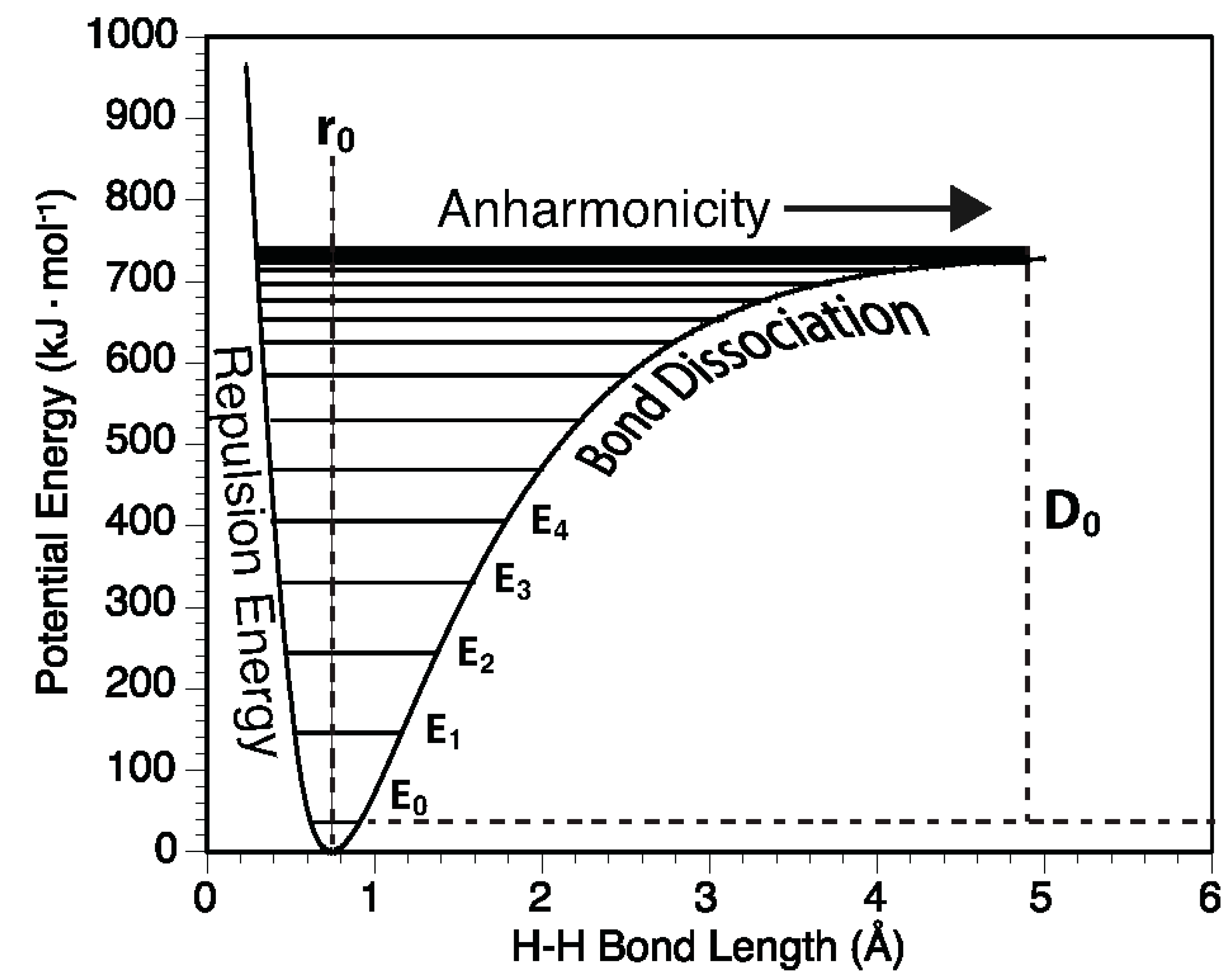
2.4. Anharmonicity

As mentioned above, many programs and methods rely upon the harmonic approximation to obtain frequencies, and this approximation is reasonably accurate in most cases. Calculation of vibrational frequencies via the velocity autocorrelation function (VACF) avoids this issue by estimating frequencies from predicted atomic motion, but this approach relies upon MD simulations of the model that may require tens of thousands of steps [24], which may not be practical in all cases (e.g., when the model system contains many atoms and quantum calculations are necessary). Anharmonic frequencies can be calculated directly in programs such as Gaussian [25], but these methods can also be time-consuming for more complex models. Calculated anharmonic frequencies can provide higher-precision overtone and combination bands, which can give calculated results that agree well with experimental frequencies; however, evidence suggests that anharmonic frequency calculations have low precision when calculated using small basis sets [26], and large basis sets could make the calculation computationally expensive (Note that the Gaussian, FREQ = Anharmonic keyword designation also provides for overtone and combination mode frequencies (

Table 1. The Gaussian 09 [18] output for a harmonic and anharmonic frequency calculation of a H₂O model at the B3LYP/6-31G(d,p) level of theory [28,29,30,31,32]. ZPE is the zero-point energy.

Mode	ν(Harm) (cm−1)	ν(Anharm) (cm−1)
Fundamental Bands
1(1)	3913.897	3726.279
2(1)	3800.402	3628.674
3(1)	1664.814	1615.055
Overtones
1(2)	7827.794	7355.593
2(2)	7600.805	7172.676
3(2)	3329.628	3193.999
Combination Bands
2(1) 1(1)	7714.299	7190.895
3(1) 1(1)	5578.711	5324.089
3(1) 2(1)	5465.217	5233.679
ZPE(Harm) = 56.10 kJ/mol  ZPE(Anharm) = 55.24 kJ/mol

), but these appear in the near-IR region of the spectrum above 4000 cm⁻¹, which is not commonly used in studies of geomaterials such as clays. That is not to say that this technique would not be useful, as it has been applied successfully to study the nature of water [27].

The most common approach has been to use scaling factors to estimate the magnitude of the anharmonicity for a given model [33], whereby each harmonic frequency is multiplied by a factor to obtain an estimated anharmonic (i.e., observed) frequency. This quick correction is so common that it is implemented in programs such as GaussView, Molden [23], and WebMO [34] as part of the spectral visualization toolkit. For the most part, scaling factors are between 0.96 and 1.0, so the method works well as a first approximation (see the National Institute of Standards and Technology Computational Chemistry Comparison and Benchmark DataBase for a compilation of scaling factors).

Unfortunately, most of these scaling factors have been developed for neutral, gas-phase molecules, so they do not account for charged species and the effects of strong solvents such as water. A researcher can determine their own scale factors for a given model, method, and range of frequencies. A straightforward approach is to select a material of known structure (e.g., illite), calculate the vibrational frequencies, and then correlate calculated and observed frequencies. This can be done over the entire mid-IR range (400 to 4000 cm⁻¹) or broken into sections such as the Al–O/Si–O stretching and O–H stretching regions to account for different anharmonicities in various bond types. To our knowledge, a detailed study of this sort has not been conducted on clays, but an example of this approach can be found in Lee et al. [35,36], who modeled the vibrational frequencies of celluloses (an ordered fibril of glucan polymers) in order to assign observed IR, Raman, and SFG peaks. It is not surprising to find different levels of anharmonicity in C–H and O–H bonds in the case of celluloses, so one should not expect a single average scale factor to work equally well for all the bond types within a complex material such as a clay.

3. Practical Considerations

In most computational chemistry studies, there is a trade-off between the accuracy of the method used and the size of the model. This is because higher-accuracy calculations are generally more computationally demanding; moreover, larger models also increase the amount of processing power and memory required to complete an electronic structure calculation. There are strategies for dealing with these limitations. First, one should build the minimal structural model necessary that includes the critical components involved. The “minimum” size depends on the question asked and the accuracy necessary. For years, many researchers performed calculations on molecules in vacuo and ignored solvent effects even when modeling aqueous reactions. This led to significant errors, but modeling a solvent is not as straightforward. For many structural and thermodynamic problems, researchers rely upon “implicit” or “continuum” models to account for the longer-range dielectric effects of solvation (e.g., polarized continuum models [37,38] or COSMO-RS [39,40,41]). Although this approach is sufficient in some cases, modeling vibrational frequencies while ignoring explicit solvation via H₂O and the potential strong H-bonding effects it could have may lead to inaccurate frequencies.

For example, a calculation in Gaussian using B3LYP/6-31G(d,p) on an H₂O molecule in vacuo results in frequencies of 1665, 3800 and 3914 cm⁻¹. Performing the energy minimization and frequency analysis with the same method in the integral equation formalism polarized continuum model (IEFPCM) [38], which is a solvent approximating technique, results in frequencies of 1664, 3799, and 3895 cm⁻¹, which is a substantial shift of almost 20 cm⁻¹ for the asymmetric O–H stretch. Adding just one more H₂O molecule to H-bond to one O atom of the original H₂O leads to corresponding frequencies of 1664/1691 (H–O–H angle bending), 3745/3767 (symmetric O–H bond stretching), and 3882 cm⁻¹ (asymmetric O–H bond stretching). One can see substantial frequency shifts and a potential for peak broadening since the similar modes at different frequencies will merge into bands as atomic motion in real systems averages these structures. (Note: one method of dealing with closely spaced frequencies of similar modes is to calculate averages weighted by either the IR- or Raman-intensities for comparison with observed peak positions.) This issue can be exacerbated in charged systems, especially when there is a deprotonated O atom that can form up to three strong H-bonds to H₂O or a nearby OH group.

Another fundamental consideration is the accuracy required of the calculation in order to answer a scientific question. Generally, agreement between calculated and observed frequencies is on the order of ±10 cm⁻¹ for geomaterials (sometimes less accurate) after scaling calculated harmonic frequencies based on the correlation with observed anharmonic frequencies. Therefore, subtle changes on the order of a few cm⁻¹ or less in a vibrational spectrum are hard to reproduce with common DFT methods. On the other hand, it is not always necessary to have a high level of accuracy when distinguishing among the probabilities of various hypothesized models. If one agrees significantly better with the overall vibrational spectrum, it is the most likely species. One can test this further by comparing to other types of observables such as EXAFS or NMR. Additionally, calculating the relative energetic stability of each model will predict which is favored and one can check for consistency with the spectral results. The user is advised to always look for the preponderance of evidence and weigh each piece according to its strength. Do not become enamored of the power of computational chemistry and the ability of a program to provide an answer and picture regarding the scientific system of interest.

4. Examples

Several examples will be discussed that examine the use of computational vibrational spectroscopy to understand clay structure and the behavior of clays with respect to adsorbates. Another example will discuss the application of DFT to probing the structure of a hydrous silica glass. Infrared and Raman spectroscopies have been the most commonly employed to study clay minerals and clay-type materials, so this work will focus on these methods. However, we encourage the reader to examine other methods such as sum-frequency generation (SFG) and inelastic neutron scattering (INS). Those techniques can provide excellent information on vibrational states of geomaterials. For a recent review of SFG, see Covert and Hore [42]. A good example of combining INS with DFT as applied to a clay can be found in Jiménez-Ruiz et al. [43].

4.1. Gibbsite

Gibbsite (Al(OH)₃) serves as a relatively simple example for modeling clays and other minerals, but the presence of the OH groups allows it to be used to illustrate principles of H-bonding and how they affect O–H vibrations. For a mineral, it generally makes sense to use a 3-D periodic calculation in a program such as VASP [44,45,46,47,48,49,50], CASTEP [51], CRYSTAl [52,53], QUANTUM ESPRESSO [54,55], or SIESTA [56]. We use VASP (5.4, VASP Software GmbH, Vienna, Austria) mainly due to its computational efficiency when performing larger scale and MD simulations, but other programs have advantages as well, so each researcher should evaluate the suite of available programs for his/her needs before starting on a project. As mentioned above, the first step is to energy minimize the system, so one chooses the exchange-correlation functional, pseudopotentials, energy cutoffs, etc., that are likely to produce reliable results. In VASP, the experimental gibbsite crystal structure [57] was energy minimized by allowing only the atoms to relax (IBRION = 2) and not the lattice parameters (i.e., ISIF = 2). Allowing the lattice parameters to relax would be a more stringent test of the accuracy of a selected DFT method, but for our purposes, it was an unnecessary step to generate model frequencies for the study of H-bonding and O–H stretches. For comparison, Al–O, O–H, and H---O (H-bond distances) from the experimental structure were 1.85, 0.88, and 1.91 Å; the DFT values were 1.86, 0.99, and 1.81 Å. The framework Al–O bonds are similar, but the O–H and H---O bond lengths are significantly different. One generally assumes that the experimental values will be more accurate, but in this case, XRD does not “see” H atoms in the structure, so the DFT-derived values are likely to be more accurate than the experimental values.

One method of testing this is to calculate the O–H vibrational frequencies and compare them to experiment. A difference of 0.1 Å would make a significant difference in the O–H frequency. Observed frequencies compared to DFT-calculated frequencies are shown below.

• Gibbsite D [58]
  3623 3526 3456 3397 3367 3290 1054 1020 967 942 915
• DFT bulk gibbsite
  3673 3666 3549 3526 3508 3494 1119 1086 1058 1041 1010 990
• DFT (001) surface gibbsite
  3866 3835 3759 3736 3668 3522 3475 1110 1066 1027 994

(Key VASP input parameters—IBRION = 5 for vibrational analysis, POTIM = 0.015 Δx, Δy, Δz, ENCUT = 500 eV energy cut-off, KPOINTS = 1 1 1 for single Γ-centered k-point)

There is a good correspondence (Figure 5) between the observed and DFT-calculated frequencies for both the O–H (3290 to 3667 cm⁻¹) and Al–O frequencies (915 to 1054 cm⁻¹). The model values are generally higher than observation due to the harmonic approximation (e.g., 3290 observed vs 3494 and 3475 cm⁻¹ calculated). One might think that the highest calculated frequencies should correspond with the highest observed frequencies, but it is known that isolated OH groups (i.e., those with no H-bond present) vibrate at approximately 3750 cm⁻¹. Hence, the higher model frequencies are due to the presence of isolated OH groups; however, this is difficult to achieve in experiment unless the sample is dried and kept dry (out of ambient atmospheric moisture) while collecting spectra. This is particularly true for the model (001) gibbsite surface where termination of the crystal leads to missing H-bonds. In a real sample, H₂O_(g) is likely to adsorb onto the surface and mimic the H-bonding normally present within the mineral. Note that an observed vibrational frequency, whether from experiment or a calculation, is generally due to the contribution of more than one vibrational mode. For example, it is unlikely that a single OH vibrational mode is responsible for a calculated or observed vibrational frequency; it is likely that multiple OH modes (and other, non-OH vibrational modes) are contributing to the frequency [59].

We note that neither IR nor Raman intensities were calculated in this exercise. Previous work on Al–O and Al–OH clusters has shown the basic principle that as H-bonding increases (i.e., shorter H---O distances), O–H bond lengths increase, O–H stretching frequencies decrease, and IR intensities increase significantly [19,60]. Hence, one needs to appreciate this correlation when analyzing the O–H stretching region of IR spectra because the lower frequency region (3000 to 3400 cm⁻¹) may represent many fewer O–H groups than the higher frequency region (3400 to 3700 cm⁻¹) because each vibrating O–H will have a larger ε (Equation (1)) value at the lower frequencies.

4.2. Birnessites

Birnessites are a form of Mn-oxide common in the environment. Mn-oxides can be critical components in the environment because they are highly reactive minerals and play a role in many biological redox processes. The reactivity is in part due to the high redox potential of Mn and in part due to the nanocrystalline nature of the Mn-oxide particles found in natural environments. Thus, Mn-oxides are small, poorly crystalline phases in soils and sediments, which makes them difficult to characterize.

Ling et al. [61] studied two main forms of birnessites, triclinic Na-birnessite (Na_0.5(Mn⁴⁺_1.42Mn³⁺_0.5)O₄∙1.5H₂O) and hexagonal H-birnessite Mn³⁺_0.12Mn²⁺_0.05 (Mn⁴⁺_0.74Mn³⁺_0.10◊_0.17)O_1.7(OH)₃ where “◊” = a vacancy). The compositional complexity of these minerals complicates identification and understanding of their chemistry. X-ray diffraction (XRD) and extended X-ray absorption fine structure (EXAFS) spectroscopy are limited in their ability to identify these fine-grained phases, so a relatively simple and inexpensive method was desired. Fourier-transform infrared (FTIR) spectroscopy was selected for this task to determine whether or not characteristic vibrational frequencies could distinguish triclinic and hexagonal birnessites.

Ling et al. [61] were able to correlate the amounts of Na-birnessite in controlled samples as determined via FTIR spectroscopy with the amounts estimated via both XRD and EXAFS. The vibrational spectra (Figure 6) were modeled with extended clusters of birnessites that attempted to mimic the triclinic birnessite and the hexagonal birnessite with and without a vacancy (Figure 7). Frequencies observed in the FTIR spectra were assigned to Mn–O vibrational modes in the two types of birnessites via analysis of the DFT calculations performed in Gaussian 09 [18]. In addition, DFT modeling of the H–O–H bending and O–H stretching region (≈1570 to 3750 cm⁻¹) frequencies and modes were used to help explain the vacancy structure where H⁺ replaces Na⁺ in the birnessite structure (Figure 6).

This example illustrates how DFT calculations can be used in combination with other techniques to decipher structures of natural materials that represent challenges for normal XRD alone. The DFT results can be compared directly with the XRD and EXAFS structural results as well as the FTIR frequencies, so one becomes more convinced that the results are not fortuitous agreements, rather than supporting evidence, which could mislead the researcher. DFT can become a powerful tool for studying chemistry at defects or other sites that occur in concentrations too low to be characterized well with typical analytical techniques. The computational chemistry approach allows one to explore various hypotheses derived from the experimental data available and make predictions where experimental data are limited. These predictions are always subject to error, but one can minimize this risk by demonstrating agreement with observable data wherever possible.

4.3. Kaolinite–Acetic Acid

Whether in soils, sediments, or suspended in the atmosphere, clay mineral surfaces are commonly decorated with adsorbed ligands. These adsorption reactions affect the interactions of clays with each other and other components in the environment. One example is that of mineral dusts that can be adsorbed organic compounds and how this affects the absorption of UV, visible, and IR radiation. These adsorbates also influence the ice-nucleation properties of a mineral aerosol, and therefore play a significant role in the Earth’s weather and climate.

As a step towards understanding and quantifying these roles in atmospheric chemistry and radiative transfer, [62] studied adsorption of acetic acid onto kaolinite surfaces using diffuse reflectance infrared Fourier-transform spectroscopy (DRIFTS) and DFT calculations to determine potential mechanisms of organic acid adsorption onto this common clay mineral. The effect of humidity on the acetic acid adsorption was observed experimentally and modeled as well to explore the effects of this critical atmospheric parameter on the expected observations.

DFT calculations were performed on a cluster representing the (100) surface of kaolinite and were based on the extended cluster created in Molina-Montes et al. [63]. A cluster, comprised of a six-membered SiO₄-tetrahedral ring and two Al-octahedra, was deemed sufficient to maintain a reasonably close approximation of the kaolinite surface. Acetic acid and acetate were bonded to the Al atoms of this cluster in various configurations (Figure 8) and subjected to energy minimizations before frequency analyses. Computed frequencies and intensities were used to correlate with observed DRIFTS data, and the best statistical fits were assigned to the surface complexes present. As is often the case [15], the spectra could not be described by the existence of a single surface complex type (Figure 9). The complex nature of the sorbates in these cases emphasizes the utility of DFT modeling of vibrational spectra because the contribution of various species can be quantitatively assessed separately rather than attempting to assign all peaks to a single surface complex.

The relative thermodynamic stability of each observed surface complex is not necessarily equal however. Often, adsorption experiments may be performed under conditions that maximize adsorption in order to obtain enough adsorbate for detection with a given technique (i.e., DRIFTS in this case). This approach is effective for obtaining structural results, but it can be misleading when one attempts to use laboratory-based adsorption in the natural world where conditions may vary significantly from the experimental conditions. Alstadt et al. [62] dealt with a significant factor for heterogeneous atmospheric chemistry, humidity, to assess its impact on the observed surface complexes. DRIFTS spectra indicated a non-uniform decrease in adsorbed acetate as a function of increasing humidity, so inner-sphere (i.e., covalently bound) acetate–kaolinite complexes were compared to H-bonded adsorbates after exchange with H₂O. Thermodynamic results (i.e., ΔG derived from DFT frequency calculations) indicated that the bidentate binuclear surface complex was the lowest in Gibbs free energy and should be the least likely to exchange with H₂O upon increasing humidity. The computed thermodynamics were consistent with observed DRIFTS data because the species most present after exposure to humidity was the surface complex assigned to the bidentate binuclear surface complex [62]. This example is another illustration where one uses a combination of DFT and vibrational spectroscopy to determine molecular configuration, but the investigator should always look for other types of data such as the thermodynamics of reactions to buttress conclusions based on DFT and vibrational spectroscopy.

4.4. Silica Species in SiO₂–H₂O Liquids and Glass

As a final example, we summarize a study by Spiekermann et al. [65] from the research group of Sandro Jahn. Vibrational spectroscopy is a useful method for probing the structure of silica in aqueous solution and of hydrous silica glasses [65]. This work used DFT molecular dynamics simulations and the mode-projection approach in the CPMD code [66] and the PBE [67] DFT method to compare and contrast the calculated results with experimental data. The authors decomposed the vibrational spectra of in the silica dimer model H₆Si₂O₇ into sub-spectra for species that included the SiO₄ tetrahedron, the Si–O–Si bridging O, and the individual Si–OH stretching.

A notable finding from this work was the discussion of the experimentally observed Raman band at 970 cm⁻¹, which has been attributed to the Si–OH stretch of a Q³ silica. In addition, experimentalists have assigned a Raman stretch at 910–915 cm⁻¹ to the Q² species. The calculations showed that Si–OH stretches occurred at 920 cm⁻¹ for Q², which agreed well with the experiment, but at 930 cm⁻¹ for Q³, which did not agree well with the experiment. Furthermore, the calculations showed Q³ stretches at 1015 and 1100 cm⁻¹, but not at 970 cm⁻¹. Therefore, the calculated results suggest that the Raman frequency at 970 cm⁻¹ might not be due to Q³ Si–OH stretches as predicted experimentally. However, the calculations did show a vibration at 970 cm⁻¹ for a Q² tetrahedral stretch that was not due to Si–OH stretching. The authors suggested further investigation to determine what is causing the Raman stretch at 970 cm⁻¹.

4.5. Further Reading

Although this section focused primarily on examples from work published by our group, myriad papers from other groups including those by Jahn et al. [68,69], Tunega et al. [70,71,72], and Balan et al. [73,74,75] are recommended.

5. Conclusions

• Make sure you are building a model that represents reality as closely as possible.
• Search the literature for previous studies for guidance as to which method will be accurate for your purposes.
• Use periodic and cluster models to complement one another; each model type has strengths and weaknesses.
• Most classical force field methods will not be as accurate as quantum methods. Many are parameterized to have bond force constants, k, obtained from experimental vibrational frequencies.
• Benchmark computational methods against well-understood systems wherever possible to estimate error in calculations.
• If possible, compare your calculated results with other sources of experimental data (e.g., NMR, XANES, EXAFS) to increase the certainty of your calculated results.

References

- Simon, J.D.; McQuarrie, D.A. The Boltzmann Factor and Partition Functions. In Physical Chemistry: A Molecular Approach; University Science Book: Sausalito, CA, USA, 1997; pp. 693–722. [Google Scholar]
- Schauble, E. Applying stable isotope fractionation theory to new systems. Rev. Mineral. Geochem. 2004, 55, 65–111. [Google Scholar] [CrossRef]
- Eiler, J.M.; Bergquist, B.; Bourg, I.; Cartigny, P.; Farquhar, J.; Gagnon, A.; Guo, W.; Halevy, I.; Hofmann, A.; Larson, T.E.; et al. Frontiers of stable isotope geoscience. Chem. Geol. 2014, 372, 119–143. [Google Scholar] [CrossRef]
- Kubicki, J.D.; Rosso, K.M. Geochemical kinetics via computational chemistry. In Molecular Modeling of Geochemical Reactions: An Introduction.; Kubicki, J.D., Ed.; Wiley: Hoboken, NJ, USA, 2016; pp. 375–414. [Google Scholar]
- Philipona, R.; Dürr, B.; Marty, C.; Ohmura, A.; Wild, M. Radiative forcing-measured at Earth’s surface-corroborate the increasing greenhouse effect. Geophys. Res. Lett. 2004, 31, L03202. [Google Scholar] [CrossRef]
- Collins, W.D.; Ramaswamy, V.; Schwarzkopf, M.D.; Sun, Y.; Portmann, R.W.; Fu, Q.; Casanova, S.E.B.; Dufresne, J.-L.; Fillmore, D.W.; Forster, P.M.D.; et al. Radiative forcing by well-mixed greenhouse gases: Estimates from climate models in the Intergovernmental Panel on Climate Change (IPCC) Fourth Assessment Report (AR4). J. Geophys. Res. 2006, 111, D14317. [Google Scholar] [CrossRef]
- Harries, J.E.; Brindley, H.E.; Sagoo, P.J.; Bantges, R.J. Increases in greenhouse forcing inferred from the outgoing longwave radiation spectra of the Earth in 1970 and 1997. Nature 2001, 410, 355–357. [Google Scholar] [CrossRef] [PubMed]
- Peters, W.; Jacobson, A.R.; Sweeney, C.; Andrews, A.E.; Conway, T.J.; Masarie, K.; Miller, J.B.; Bruhwiler, L.M.P.; Pétron, G.; Hirsch, A.I.; et al. An atmospheric perspective on North American carbon dioxide exchange: CarbonTracker. Proc. Natl. Acad. Sci. USA 2007, 104, 18925–18930. [Google Scholar] [CrossRef] [PubMed]
- IPCC. Climate Change 2007: Working Group I: The Physical Science Basis Contribution of Working Group I to the Fourth Assessment Report of the Intergovernmental Panel on Climate Change, 2007; Cambridge University Press: Cambridge, UK, 2007. [Google Scholar]
- Morman, S.A.; Plumlee, G.S. The role of airborne mineral dusts in human disease. Aeolian Res. 2013, 9, 203–212. [Google Scholar] [CrossRef]
- Fröhlich-Nowoisky, J.; Kampf, C.J.; Weber, B.; Huffman, J.A.; Pöhlker, C.; Andreae, M.O.; Lang-Yona, N.; Burrows, S.M.; Gunthe, S.S.; Elbert, W.; et al. Bioaerosols in the Earth system: Climate, health, and ecosystem interactions. Atmos. Res. 2016, 182, 346–376. [Google Scholar] [CrossRef]
- Groot Zwaaftink, C.D.; Grythe, H.; Skov, H.; Stohl, A. Substantial contribution of northern high-latitude sources to mineral dust in the Arctic. J. Geophys. Res. 2016, 121, 13678–13697. [Google Scholar] [CrossRef]
- Prospero, J.M.; Collard, F.X.; Molinié, J.; Jeannot, A. Characterizing the annual cycle of African dust transport to the Caribbean Basin and South America and its impact on the environment and air quality. Glob. Biogeochem. Cycle. 2014, 28, 757–773. [Google Scholar] [CrossRef]
- Kubicki, J.D.; Sykes, D. Molecular orbital calculations of vibrations in three-membered aluminosilicate rings. Phys. Chem. Miner. 1993, 19, 381–391. [Google Scholar] [CrossRef]
- Kubicki, J.D.; Paul, K.W.; Kabalan, L.; Zhu, Q.; Mrozik, M.K.; Aryanpour, M.; Pierre-Louis, A.M.; Strongin, D.R. ATR-FTIR and density functional theory study of the structures, energetics, and vibrational spectra of phosphate adsorbed onto goethite. Langmuir 2012, 28, 14573–14587. [Google Scholar] [CrossRef] [PubMed]
- Kumar, N.; Neogi, S.; Kent, P.R.C.; Bandura, A.V.; Kubicki, J.D.; Wesolowski, D.J.; Cole, D.; Sofo, J.O. Hydrogen Bonds and Vibrations of Water on (110) Rutile. J. Phys. Chem. C 2009, 113, 13732–13740. [Google Scholar] [CrossRef]
- Yamaguchi, Y.; Frisch, M.; Gaw, J.; Schaefer, H.F.; Binkley, J.S. Analytic evaluation and basis set dependence of intensities of infrared spectra. J. Chem. Phys. 1986, 84, 2262–2278. [Google Scholar] [CrossRef]
- Frisch, M.J.; Trucks, G.W.; Schlegel, H.B.; Scuseria, G.E.; Robb, M.A.; Cheeseman, J.R.; Montgomery, A., Jr.; Vreven, T.; Kudin, K.N.; Burant, J.C.; et al. Gaussian 09 Revision E.01. Wallingford, CT. 2009. Available online: http://gaussian.com/ (accessed on 15 January 2019).
- Kubicki, J.; Sykes, D.; Rossman, G.R. Calculated Trends of OH Infrared Stretching Vibrations with Composition and Structure in Aluminosilicate Molecules. Phys. Chem. Miner. 1993, 20, 425–432. [Google Scholar] [CrossRef]
- Radom, L.; Schleyer, P.V.R.; Pople, J.A.; Hehre, W.J. Ab Initio Molecular Orbital Theory; John Wiley and Sons: San Francisco, CA, USA, 1986. [Google Scholar]
- Ogilvie, J.F. The Vibrational and Rotational Spectrometry of Diatomic Molecules; Academic Press: San Diego, CA, USA, 1998. [Google Scholar]
- Paterson, M.S. The Determination of Hydroxyl by Infrared Absorption in Quartz, Silicate Glasses and Similar Minerals. Bull. Minéral. 1982, 105, 20–29. [Google Scholar]
- Schaftenaar, G.; Noordik, J.H. Molden: A pre- and post-processing program for molecular and electronic structures. J. Comput. Aided. Mol. Des. 2000, 14, 123–134. [Google Scholar] [CrossRef] [PubMed]
- Borah, S.; Padma Kumar, P. Ab initio molecular dynamics investigation of structural, dynamic and spectroscopic aspects of Se(VI) species in the aqueous environment. Phys. Chem. Chem. Phys. 2016, 18, 14561–14568. [Google Scholar] [CrossRef] [PubMed]
- Bloino, J.; Barone, V. A second-order perturbation theory route to vibrational averages and transition properties of molecules: General formulation and application to infrared and vibrational circular dichroism spectroscopies. J. Chem. Phys. 2012, 136. [Google Scholar] [CrossRef] [PubMed]
- Jacobsen, R.L.; Johnson, R.D.; Irikura, K.K.; Kacker, R.N. Anharmonic vibrational frequency calculations are not worthwhile for small basis sets. J. Chem. Theory Comput. 2013, 9, 951–954. [Google Scholar] [CrossRef] [PubMed]
- Newman, S.; Stolper, E.M.; Epstein, S. Measurement of water in rhyolitic glasses-calibration of an infrared spectroscopic technique. Am. Mineral. 1986, 71, 1527–1541. [Google Scholar]
- Hehre, W.J.; Ditchfield, R.; Pople, J.A. Self—Consistent Molecular Orbital Methods. XII. Further Extensions of Gaussian—Type Basis Sets for Use in Molecular Orbital Studies of Organic Molecules. J. Chem. Phys. 1972, 56, 2257–2261. [Google Scholar] [CrossRef]
- Becke, A.D. Becke’s three parameter hybrid method using the LYP correlation functional. J. Chem. Phys. 1993, 98, 5648–5652. [Google Scholar] [CrossRef]
- Vosko, S.H.; Wilk, L.; Nusair, M. Accurate spin-dependent electron liquid correlation energies for local spin density calculations: A critical analysis. Can. J. Phys. 1980, 58, 1200–1211. [Google Scholar] [CrossRef]
- Stephens, P.J.; Devlin, F.J.; Chabalowski, C.; Frisch, M.J. Ab initio calculation of vibrational absorption and circular dichroism spectra using density functional force fields. J. Phys. Chem. 1994, 98, 11623–11627. [Google Scholar] [CrossRef]
- Lee, C.; Yang, W.; Parr, R.G. Development of the Colle-Salvetti correlation-energy formula into a functional of the electron density. Phys. Rev. B 1988, 37, 785–789. [Google Scholar] [CrossRef]
- Wong, M.W. Vibrational frequency prediction using density functional theory. Chem. Phys. Lett. 1996, 256, 391–399. [Google Scholar] [CrossRef]
- Schmidt, J.R.; Polik, W.F. WebMO Enterprise, Version 13.0; WebMO LLC: Holland, MI, USA, 2013. [Google Scholar]
- Lee, C.M.; Kubicki, J.D.; Fan, B.; Zhong, L.; Jarvis, M.C.; Kim, S.H. Hydrogen-Bonding Network and OH Stretch Vibration of Cellulose: Comparison of Computational Modeling with Polarized IR and SFG Spectra. J. Phys. Chem. B 2015, 119, 15138–15149. [Google Scholar] [CrossRef] [PubMed]
- Lee, C.M.; Mohamed, N.M.A.; Watts, H.D.; Kubicki, J.D.; Kim, S.H. Sum-frequency-generation vibration spectroscopy and density functional theory calculations with dispersion corrections (DFT-D2) for cellulose Iα and Iβ. J. Phys. Chem. B 2013, 117, 6681–6692. [Google Scholar] [CrossRef] [PubMed]
- Gogonea, V. Self-Consistent Reaction Field Methods: Cavities. In Encyclopedia of Computational Chemistry; von Rague Schleyer, P., Allinger, N.L., Clark, T., Gastiger, J., Kollman, P.A., Schaefer, H.F.I., Schreiner, P.R., Eds.; Wiley: New York, NY, USA, 1998; pp. 2560–2574. [Google Scholar]
- Mennucci, B.; Cancès, E.; Tomasi, J. Evaluation of Solvent Effects in Isotropic and Anisotropic Dielectrics and in Ionic Solutions with a Unified Integral Equation Method: Theoretical Bases, Computational Implementation, and Numerical Applications. J. Phys. Chem. B 1997, 101, 10506–10517. [Google Scholar] [CrossRef]
- Delley, B. The conductor-like screening model for polymers and surfaces. Mol. Simul. 2006, 32, 117–123. [Google Scholar] [CrossRef]
- Klamt, A.; Schüürmann, G. COSMO: A new approach to dielectric screening in solvents with explicit expressions for the screening energy and its gradient. J. Chem. Soc. Perkin Trans. 2 1993, 799–805. [Google Scholar] [CrossRef]
- Klamt, A.; Jonas, V.; Bürger, T.; Lohrenz, J.C.W. Refinement and Parametrization of COSMO-RS. J. Phys. Chem. A 1998, 102, 5074–5085. [Google Scholar] [CrossRef]
- Covert, P.A.; Hore, D.K. Geochemical Insight from Nonlinear Optical Studies of Mineral–Water Interfaces. Annu. Rev. Phys. Chem. 2016, 67, 233–257. [Google Scholar] [CrossRef] [PubMed]
- Jimenez-Ruiz, M.; Ferrage, E.; Blanchard, M.; Fernandez-Castanon, J.; Delville, A.; Johnson, M.R.; Michot, L.J. Combination of Inelastic Neutron Scattering Experiments and Ab-Initio Quantum Calculations for the Study of the Hydration Properties of Oriented Saponites. J. Phys. Chem. C 2017, 121, 5029–5040. [Google Scholar] [CrossRef]
- Kresse, G.; Hafner, J. Ab initio molecular dynamics for open-shell transition metals. Phys. Rev. B. Condens. Matter 1993, 48, 13115–13118. [Google Scholar] [CrossRef] [PubMed]
- Kresse, G.; Hafner, J. Ab initio molecular-dynamics simulation of the liquid-metal-amorphous-semiconductor transition in germanium. Phys. Rev. B 1994, 49, 14251–14269. [Google Scholar] [CrossRef]
- Kresse, G.; Furthmüller, J. Efficient iterative schemes for ab initio total-energy calculations using a plane-wave basis set. Phys. Rev. B 1996, 54, 11169–11186. [Google Scholar] [CrossRef]
- Kresse, G.; Furthmüller, J. Efficiency of ab-initio total energy calculations for metals and semiconductors using a plane-wave basis set. Comput. Mater. Sci. 1996, 6, 15–50. [Google Scholar] [CrossRef]
- Kresse, G.; Furthmüller, J.; Hafner, J. Theory of the crystal structures of selenium and tellurium: The effect of generalized-gradient corrections to the local-density approximation. Phys. Rev. B 1994, 50, 13181–13185. [Google Scholar] [CrossRef]
- Kresse, G.; Joubert, D. From ultrasoft pseudopotentials to the projector augmented-wave method. Phys. Rev. B 1999, 59, 1758–1775. [Google Scholar] [CrossRef]
- Blöchl, P.E. Projector augmented-wave method. Phys. Rev. B 1994, 50, 17953–17979. [Google Scholar] [CrossRef]
- Clark, S.J.; Segall, M.D.; Pickard, C.J.; Hasnip, P.J.; Probert, M.I.J.; Refson, K.; Payne, M.C. First principles methods using CASTEP. Z. Krist. Cryst. Mater. 2005, 220, 567–570. [Google Scholar] [CrossRef]
- Dovesi, R.; Erba, A.; Orlando, R.; Zicovich-Wilson, C.M.; Civalleri, B.; Maschio, L.; Rérat, M.; Casassa, S.; Baima, J.; Salustro, S.; et al. Quantum-mechanical condensed matter simulations with CRYSTAL. WIREs Comput. Mol. Sci. 2018, 8, e1360. [Google Scholar] [CrossRef]
- Pascale, F.; Zicovich-Wilson, C.M.; López Gejo, F.; Civalleri, B.; Orlando, R.; Dovesi, R. The calculation of the vibrational frequencies of crystalline compounds and its implementation in the CRYSTAL code. J. Comput. Chem. 2004, 25, 888–897. [Google Scholar] [CrossRef] [PubMed]
- Giannozzi, P.; Baroni, S.; Bonini, N.; Calandra, M.; Car, R.; Cavazzoni, C.; Ceresoli, D.; Chiarotti, G.L.; Cococcioni, M.; Dabo, I.; et al. QUANTUM ESPRESSO: A modular and open-source software project for quantum simulations of materials. J. Phys. Condens. Matter 2009, 21, 395502. [Google Scholar] [CrossRef] [PubMed]
- Giannozzi, P.; Andreussi, O.; Brumme, T.; Bunau, O.; Buongiorno Nardelli, M.; Calandra, M.; Car, R.; Cavazzoni, C.; Ceresoli, D.; Cococcioni, M.; et al. Advanced capabilities for materials modelling with Quantum ESPRESSO. J. Phys. Condens. Matter 2017, 29, 465901. [Google Scholar] [CrossRef] [PubMed]
- Soler, J.M.; Artacho, E.; Gale, J.D.; Garcia, A.; Junquera, J.; Ordejon, P.; Sanchez-Portal, D. The SIESTA method for ab initio order-N materials simulation. J. Phys. Condens. Matter 2001, 14, 2745–2779. [Google Scholar] [CrossRef]
- Saalfeld, H.; Wedde, M. Refinement of the crystal structure of gibbsite, Al(OH)3. Z. Krist. Cryst. Mater. 1974, 139, 120–135. [Google Scholar] [CrossRef]
- Frost, R.A.Y.L.; Kloprogge, J.T.; Russell, S.C.; Szetu, J.L. Vibrational Spectroscopy and Dehydroxylation of Aluminum (Oxo) hydroxides: Gibbsite. Appl. Spectrosc. 1999, 53, 423–434. [Google Scholar] [CrossRef]
- Balan, E.; Lazzeri, M.; Morin, G.; Mauri, F. First-principles study of the OH-stretching modes of gibbsite. Am. Mineral. 2006, 91, 115–119. [Google Scholar] [CrossRef]
- Kubicki, J.D.; Apitz, S.E. Molecular cluster models of aluminum oxide and aluminum hydroxide surfaces. Am. Mineral. 1998, 83, 1054–1066. [Google Scholar] [CrossRef]
- Ling, F.T.; Post, J.E.; Heaney, P.J.; Kubicki, J.D.; Santelli, C.M. Fourier-transform infrared spectroscopy (FTIR) analysis of triclinic and hexagonal birnessites. Spectroc. Acta Pt. A Molec. Biomolec. Spectr. 2017, 178, 32–46. [Google Scholar] [CrossRef] [PubMed]
- Alstadt, V.J.; Kubicki, J.D.; Freedman, M.A. Competitive Adsorption of Acetic Acid and Water on Kaolinite. J. Phys. Chem. A 2016, 120, 8339–8346. [Google Scholar] [CrossRef] [PubMed]
- Molina-Montes, E.; Timón, V.; Hernández-laguna, A.; Sainz-díaz, C.I. Dehydroxylation mechanisms in Al3+/Fe3+ dioctahedral phyllosilicates by quantum mechanical methods with cluster models. Geochim. Cosmochim. Acta 2008, 72, 3929–3938. [Google Scholar] [CrossRef]
- Zhao, Y.; Schultz, N.E.; Truhlar, D.G. Design of Density Functionals by Combining the Method of Constraint Satisfaction with Parametrization for Thermochemistry, Thermochemical Kinetics, and Noncovalent Interactions. J. Chem. Theory Comput. 2006, 2, 364–382. [Google Scholar] [CrossRef] [PubMed]
- Spiekermann, G.; Steele-Macinnis, M.; Schmidt, C.; Jahn, S. Vibrational mode frequencies of silica species in SiO₂-H₂O liquids and glasses from ab initio molecular dynamics. J. Chem. Phys. 2012, 136, 154501. [Google Scholar] [CrossRef] [PubMed]
- Marx, D.; Hutter, J. Modern Methods and Algorithms of Quantum Chemistry. Forsch. Jülich NIC Ser. 2000, 1, 301–449. [Google Scholar]
- Perdew, J.; Burke, K.; Ernzerhof, M. Generalized gradient approximation made simple. Phys. Rev. Lett. 1996, 77, 3865–3868. [Google Scholar] [CrossRef] [PubMed]
- Spiekermann, G.; Steele-MacInnis, M.; Kowalski, P.M.; Schmidt, C.; Jahn, S. Vibrational properties of silica species in MgO-SiO₂ glasses obtained from ab initio molecular dynamics. Chem. Geol. 2013, 346, 22–33. [Google Scholar] [CrossRef]
- Spiekermann, G.; Steele-MacInnis, M.; Kowalski, P.M.; Schmidt, C.; Jahn, S. Vibrational mode frequencies of H4SiO4, D4SiO4, H6Si2O7, and H6Si3O9 in aqueous environment, obtained from ab initio molecular dynamics. J. Chem. Phys. 2012, 137, 164506. [Google Scholar] [CrossRef] [PubMed]
- Scholtzová, E.; Madejová, J.; Jankovič, L.; Tunega, D. Structural and spectroscopic characterization of montmorillonite intercalated with N-butylammonium cations (N = 1–4)-Modeling and experimental study. Clay. Clay Miner. 2016, 64, 401–412. [Google Scholar] [CrossRef]
- Tunega, D.; Benco, L.; Haberhauer, G.; Gerzabek, M.H.; Lischka, H. Ab initio molecular dynamics study of adsorption sites on the (001) surfaces of 1:1 dioctahedral clay minerals. J. Phys. Chem. B 2002, 106, 11515–11525. [Google Scholar] [CrossRef]
- Scholtzová, E.; Tunega, D.; Madejová, J.; Pálková, H.; Komadel, P. Theoretical and experimental study of montmorillonite intercalated with tetramethylammonium cation. Vib. Spectrosc. 2013, 66, 123–131. [Google Scholar] [CrossRef]
- Balan, E.; Lazzeri, M.; Saitta, A.M.; Allard, T.; Fuchs, Y.; Mauri, F. First-principles study of OH-stretching modes in kaolinite, dickite, and nacrite. Am. Mineral. 2005, 90, 50–60. [Google Scholar] [CrossRef]
- Balan, E.; Saitta, A.M.; Mauri, F.; Calas, G. First-principles modeling of the infrared spectrum of kaolinite. Am. Mineral. 2001, 86, 1321–1330. [Google Scholar] [CrossRef]
- Balan, E.; Saitta, A.M.; Mauri, F.; Lemaire, C.; Guyot, F. First-principles calculation of the infrared spectrum of lizardite. Am. Mineral. 2002, 87, 1286–1290. [Google Scholar] [CrossRef]