Spatial Chirp of Agate Bands


Abstract
:1. Introduction
2. Materials and Methods
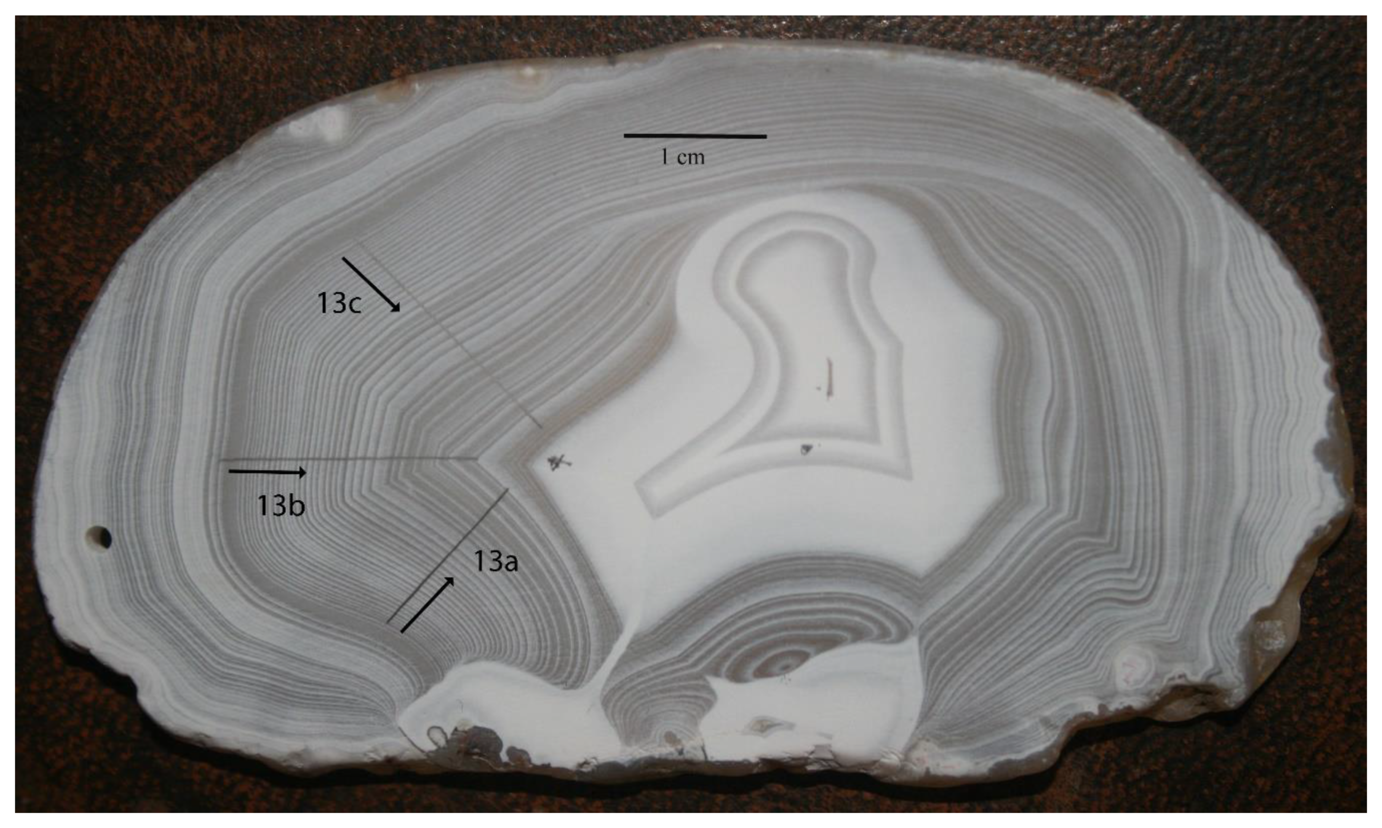
2.1. Materials
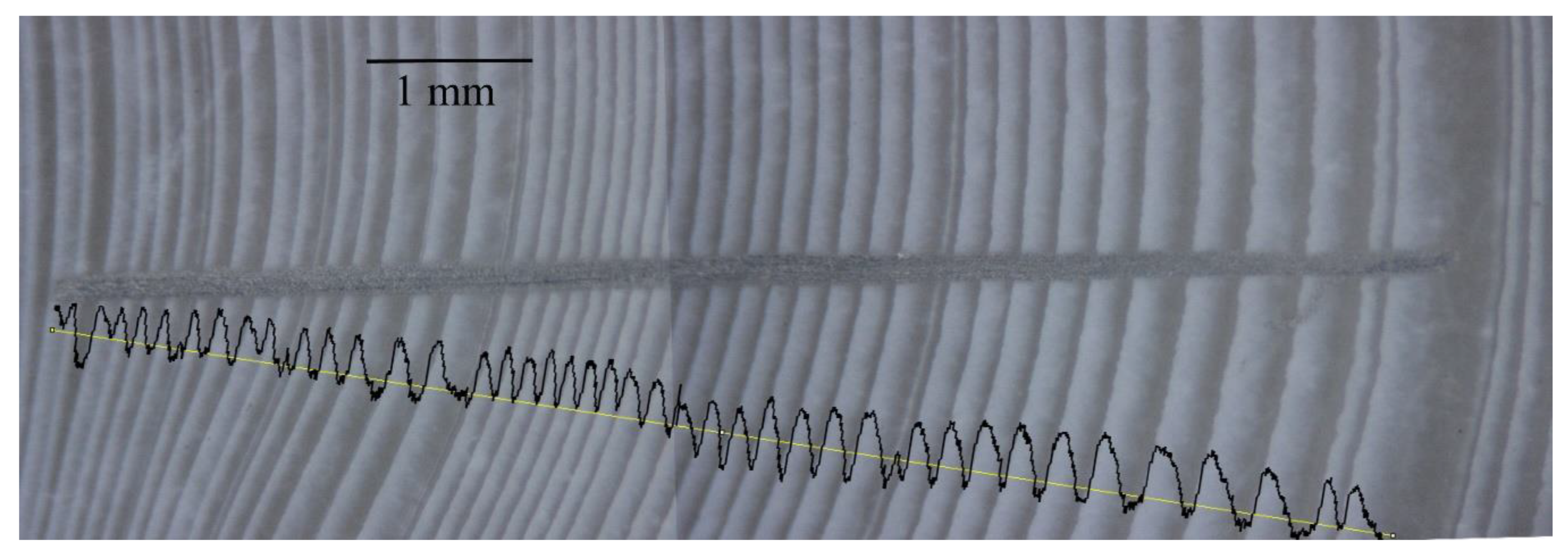
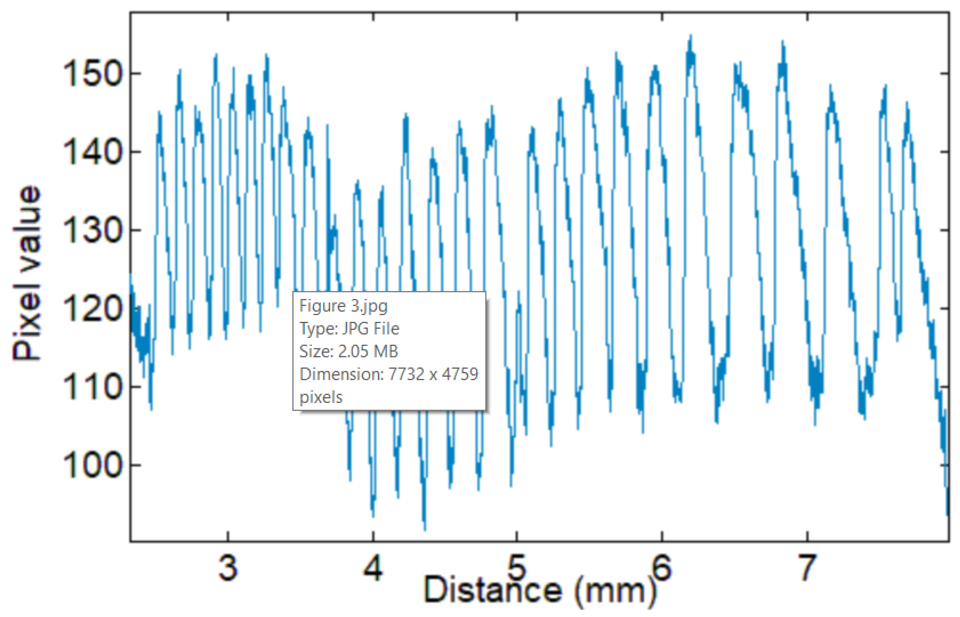
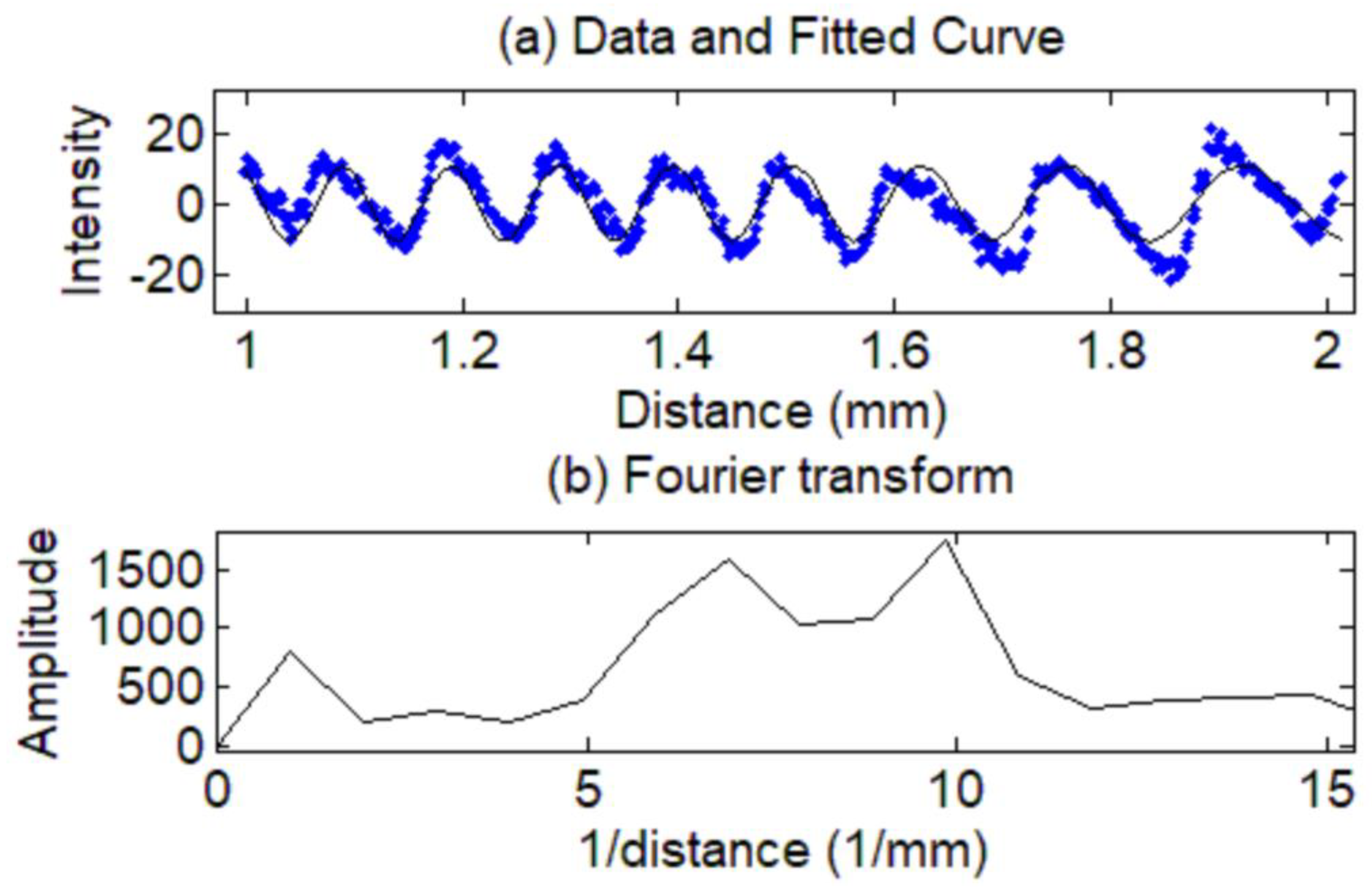
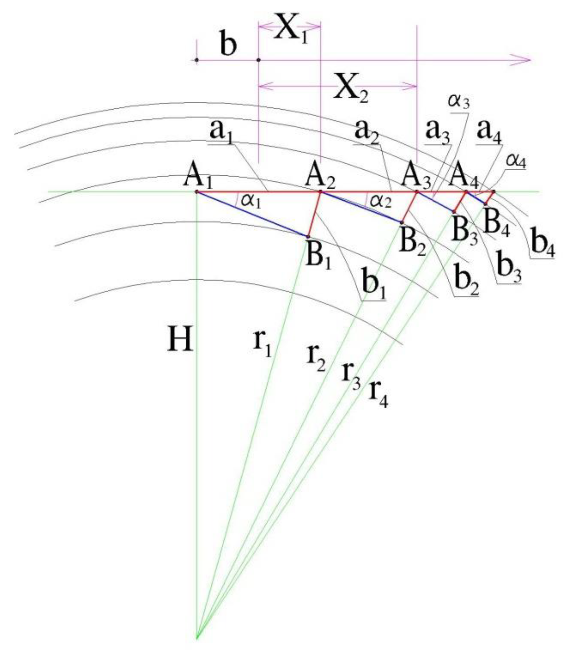
2.2. Analysis
- The lines A1B1, A2B2 etc. are approximately tangent to the circles. Hence:
- The angles A1B1A2 etc. are approximately 90°, and
- The angles B1A1A2 etc. i.e., α, α’ etc. are approximately equal.
3. Results
4. Discussion
5. Conclusions
Author Contributions
Funding
Conflicts of Interest
References
- Götze, J.; Berek, H.; Schäfer, K. Micro-structural phenomena in agate/chalcedony: Spiral growth. Mineral. Mag. 2019, 83, 281–291. [Google Scholar] [CrossRef]
- Richter-Feig, J.; Möckel, R.; Götze, J.; Heide, G. Investigation of fluids in macrocrystalline and microcrystalline quartz in agate using thermogravimetry-mass-spectrometry. Minerals 2018, 8, 72. [Google Scholar] [CrossRef]
- Cidade, M.K.; Palombini, F.L.; Duarte, L.C.; Paciornik, S. Investigation of the thermal microstructural effects of CO2 laser engraving on agate via X-ray microtomography. Opt. Laser Technol. 2018, 104, 56–64. [Google Scholar] [CrossRef]
- Dumańska-Słowik, M.; Powolny, T.; Sikorska-Jaworowska, M.; Gaweł, A.; Kogut, L.; Poloński, K. Characteristics and origin of agates from Płóczki Górne (Lower Silesia, Poland): A combined microscopic, micro-Raman, and cathodoluminescence study. Spectrochim Acta Part A: Mol. Biomol. Spectrosc. 2018, 192, 6–15. [Google Scholar] [CrossRef] [PubMed]
- Howard, C.B.; Rabinovitch, A. A new model of agate geode formation based on a combination of morphological features and silica sol–gel experiments. Eur. J. Mineral. 2018, 30, 97–106. [Google Scholar] [CrossRef]
- Schindelin, J.; Arganda-Carreras, I.; Frise, E. Fiji: An open-source platform for biological-image analysis. Nat. Methods 2012, 9, 676–682. [Google Scholar] [CrossRef] [PubMed]
- Djurović, I.; Simeunović, M.; Wang, P. Cubic phase function: A simple solution to polynomial phase signal analysis. Signal Process. 2017, 135, 48–66. [Google Scholar] [CrossRef]
- Li, D.; Gui, X.; Liu, H.; Su, J.; Xiong, H. An ISAR imaging algorithm for maneuvering targets with low SNR based on parameter estimation of multicomponent quadratic FM signals and nonuniform FFT. Appl. Earth Obs. Remote Sens. 2016, 9, 5688–5702. [Google Scholar] [CrossRef]
- Klauder, J.R.; Price, A.C.; Darlington, S.; Albersheim, W.J. The theory and design of chirp radars. Bell Syst. Tech. J. 1960, 39, 745–809. [Google Scholar] [CrossRef]
- Flandrin, P. Time frequency and chirps. In Proceedings of the Wavelet Applications VIII, Orlando, FL, USA, 26 March 2001; International Society for Optical Photonics: Cardiff, Wales, 2001; Volume 4391, pp. 161–175. [Google Scholar] [CrossRef]
- Wang, Y.; Merino, E. Self-organizational origin of agates: Banding, fiber twisting, composition, and dynamic crystallization model. Geochim. Cosmochim. Acta 1990, 54, 1627. [Google Scholar] [CrossRef]
- Moxon, T.; Reed, S.J.B. Agate and chalcedony from igneous and sedimentary hosts aged from 13 to 3480 Ma: A cathodoluminescence study. Mineral. Mag. 2006, 70, 485–498. [Google Scholar] [CrossRef]
- Möckel, R.; Götze, J.; Sergeev, S.A.; Kapitonov, I.N.; Adamskaya, E.V.; Goltsin, N.A.; Vennemann, T. Trace-element analysis by laser ablation inductively coupled plasma mass spectrometry (LA-ICP-MS). J. Siberian Federal Univ. Eng. Technol. 2009, 2, 123–138. [Google Scholar]
- Zenz, J. Agates III; Bode Verlag: Lauenstein, Germany, 2011; p. 69. [Google Scholar]
- Grzybowski, B.A.; Bishop, K.J.M.; Campbell, C.J.; Fialkowski, M.; Smoukov, S.K. Micro- and nanotechnology via reaction-diffusion. Soft Matter 2005, 1, 114–128. [Google Scholar] [CrossRef]
- Mikhailov, A.S.; Showalter, K. Control of waves, patterns and turbulence in chemical systems. Phys. Rep. 2006, 425, 79–194. [Google Scholar] [CrossRef]
- Hongwei, Z.; Enxiang, L.; Zhaohui, Z.; Xiaobin, D.; Yuxing, P. Smart polymers based on belousov-zhabotinsky reaction. Prog. Chem. 2011, 23, 2368–2376. [Google Scholar]
- Kumar, D.K.; Steed, J.W. Supramolecular gel phase crystallization: Orthogonal self-assembly under non-equilibrium conditions. Chem. Soc. Revs. 2014, 43, 2080–2088. [Google Scholar] [CrossRef] [PubMed]

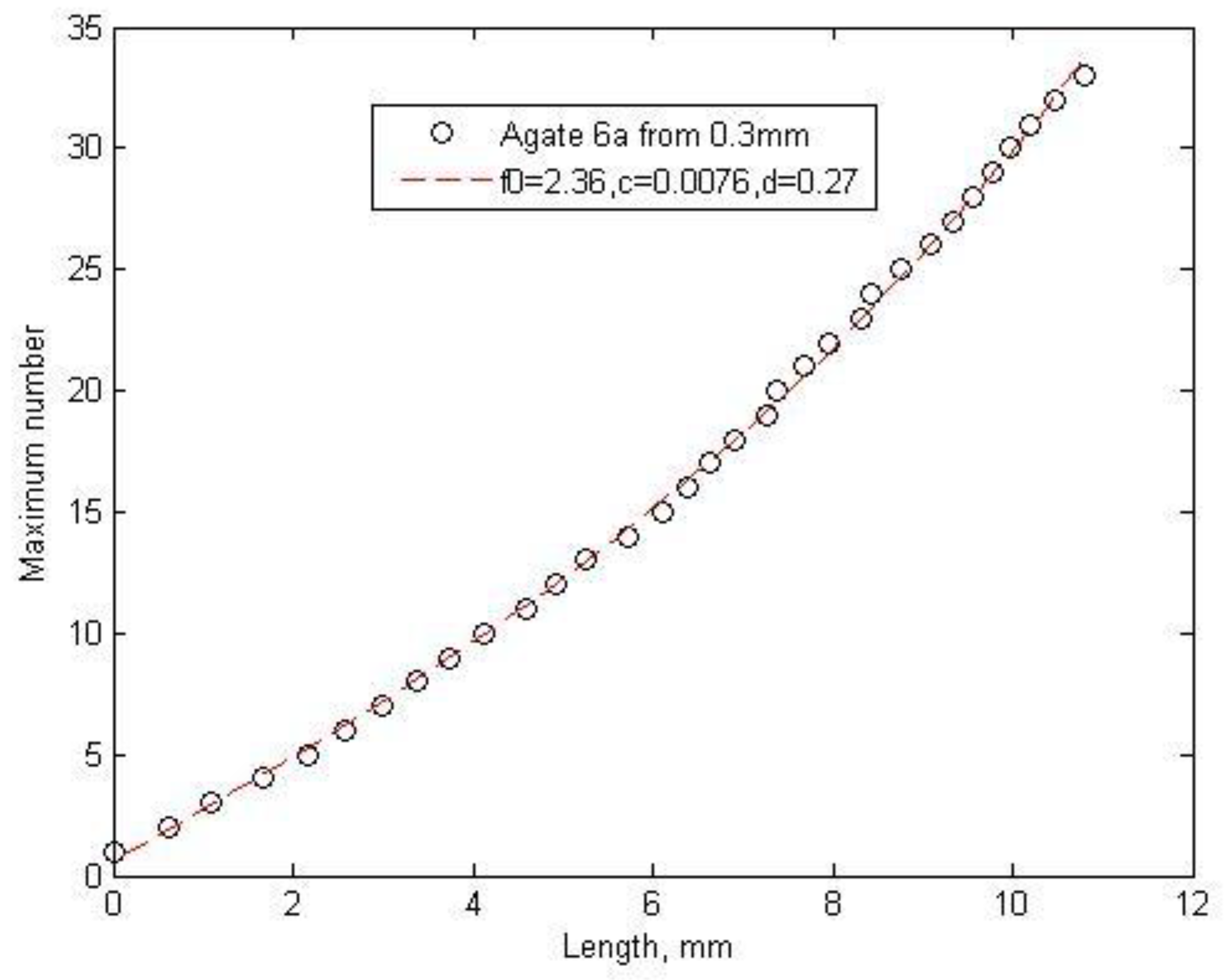
| Sample No. | Origin | Range | f0, Initial Frequency | C, Frequency Change Speed | d,mm (α = 2) | Distance between Maxima, 1/f0 | R2 |
|---|---|---|---|---|---|---|---|
| 1C | Madagascar | From 1.5 mm to end | 1.21 | 0.0066 | 1.004 | 0.82645 | 0.9924 |
| 1A | Madagascar | From 3 mm to end | 2.02 | 0.0095 | 0.27 | 0.49505 | 0.9967 |
| 1A | Madagascar | All | 1.86 | 0.0051 | 0.15 | 0.53763 | 0.9983 |
| 11B | Madagascar | To 3.5 mm | 1 | 0.0824 | 0.85 | 1 | 0.9765 |
| 13B | Madagascar | All | 2.52 | 0.0083 | 0.17 | 0.39683 | 0.9979 |
| 13B | Madagascar | From 1.3 mm to end | 3 | 0.01 | 0.05 | 0.33333 | 0.997 |
| 15 | Madagascar | All | 2.39 | 0.001 | 0.1 | 0.41841 | 0.9963 |
| 6A | Madagascar | All | 2.32 | 0.007 | 0.45 | 0.43103 | 0.9993 |
| 6A | Madagascar | From 0.3mm | 2.36 | 0.0076 | 0.27 | 0.42373 | 0.9992 |
| 7A | Madagascar | All | 1.81 | 0.0036 | 1.35 | 0.55249 | 0.9983 |
| 7A | Madagascar | From 1.5mm | 1.94 | 0.005 | 0.5 | 0.51546 | 0.9983 |
| 12 | Madagascar | All | 3 | 0.0191 | 0.59 | 0.33333 | 0.9931 |
| 12A | Madagascar | From 1.25 to 7.4 mm | 2.46 | 0.0437 | 0.6 | 0.4065 | 0.9939 |
| 12B | Madagascar | From 2.5 to 7 mm | 2.82 | 0.0977 | 0.22 | 0.35461 | 0.9932 |
| 9 | Madagascar | All | 2.74 | 0.001 | 1.39 | 0.36496 | 0.9896 |
| 20 | Botswana | All | 4.8 | 0.14 | 0.05 | 0.20833 | 0.9991 |
| 20 | Botswana | From 0.53 mm | 5.14 | 0.179 | 0.126 | 0.19455 | 0.9987 |
| 21 | Botswana | All | 5.3 | 0.006 | 0.043 | 0.18868 | 0.9959 |
| 21 | Botswana | From 3.7 mm | 1.32 | 0.864 | 0.64 | 0.75758 | 0.9981 |
| 22 | Botswana | From 3 to 6.5 mm | 1.86 | 0.0477 | 0.43 | 0.53763 | 0.9921 |
| 22 | Botswana | From 3 mm | 2.56 | 0.0018 | 0.11 | 0.39063 | 0.9848 |
| 25 | Australia | All | 3.13 | 0.01 | 0.52 | 0.31949 | 0.9913 |
| 25 | Australia | From 1.3 mm | 2.54 | 0.027 | 0.64 | 0.3937 | 0.9922 |
| 25 | Australia | From 1.9 mm | 2.42 | 0.039 | 0.6 | 0.41322 | 0.9914 |
| 25 | Australia | From 3.1 mm | 2.19 | 0.091 | 0.47 | 0.45662 | 0.9892 |
| 26 | Australia | All | 2.83 | 0.08 | 0.28 | 0.35336 | 0.9971 |
| 26 | Australia | From 0.28 mm | 2.84 | 0.098 | 0.24 | 0.35211 | 0.9967 |
| 26 | Australia | From 1.9 mm | 3.98 | 0.227 | 0.188 | 0.25126 | 0.9988 |
© 2019 by the authors. Licensee MDPI, Basel, Switzerland. This article is an open access article distributed under the terms and conditions of the Creative Commons Attribution (CC BY) license (http://creativecommons.org/licenses/by/4.0/).
Share and Cite
Goldbaum, J.; Howard, C.; Rabinovitch, A. Spatial Chirp of Agate Bands. Minerals 2019, 9, 634. https://doi.org/10.3390/min9100634
Goldbaum J, Howard C, Rabinovitch A. Spatial Chirp of Agate Bands. Minerals. 2019; 9(10):634. https://doi.org/10.3390/min9100634
Chicago/Turabian StyleGoldbaum, Julia, Charles Howard, and Avinoam Rabinovitch. 2019. "Spatial Chirp of Agate Bands" Minerals 9, no. 10: 634. https://doi.org/10.3390/min9100634
APA StyleGoldbaum, J., Howard, C., & Rabinovitch, A. (2019). Spatial Chirp of Agate Bands. Minerals, 9(10), 634. https://doi.org/10.3390/min9100634