Geometallurgical Approach to the Element-to-Mineral Conversion for the Nabbaren Nepheline Syenite Deposit

Abstract

Nabbaren nepheline syenite, a silica-deficient intrusive rock with low Fe content, was the industrial mineral deposit study case in this study. The quality of industrial mineral products are generally based on their bulk chemistry, which are directly related to their modal mineralogy and mineral chemistry; however, these are costly and time-consuming to determine. A geometallurgical-based methodology, known as element-to-mineral conversion (EMC), was applied to estimate its modal mineralogy based on its given bulk and mineral chemistry. EMC is a convenient and cost-effective technique, which can be used to quickly estimate modal mineralogy. Two EMC methodologies were applied: one least square based, LS-XRD, and one regression based, R-XRD. Additionally, average and specific mineral chemistries were used during estimations. The R-XRD method, a method not yet used for EMC purposes, gave better modal mineralogy estimations than LS-XRD. Considering the restrictions in the method, R-XRD shows potential for improvement and implementation at operational scale, making it a valuable geometallurgical tool for increasing resource performance, easing decision-taking processes, and reducing risks. The use of different mineral chemistries did not influence the modal mineralogy estimation, unlike the method used for it.

1. Introduction

The industrial minerals sector has grown and diversified in the mining industry at both regional and global scales [1,2,3,4]. In contrast to metallic ores, industrial minerals, as a mineral or a group of minerals, are mined not for their metallic content but for their physical and chemical properties [1,5]. Due to their intrinsic characteristics, most industrial minerals are used in their raw form which allows wide product variability strictly tied to consumer specifications [1].

Nepheline syenite is a silica-deficient intrusive rock, which when processed into a low-Fe feldspar-nepheline may become a commercial industrial mineral. Practical applications as a raw material include glass, ceramics, flatware manufacturing, and as pigment and filler [6]. The world leading nepheline syenite producers are Russia, Canada, and Norway with roughly 84, 10, and 6% of the world’s production, respectively [4,7]. The information used to define the industrial mineral quality relates to consumer specifications: minimum SiO₂ wt %, maximum Fe₂O₃ wt % or whiteness, among others [8].

Geometallurgy is a holistic mining-oriented discipline that incorporates information from the whole mining value chain to increase resource performance and reduce risks [9,10,11]. The ultimate goal of geometallurgy is to generate quantitative georeferenced data, which can be integrated into the 3D model and production plan of the mine [12,13]. To assess quantitative data, prediction models can be developed for operational purposes [14,15,16]. These models aim to predict multiple rock characteristics and processing behavior, and are usually restricted to the modal mineralogy of the rock. Modal mineralogy prediction is commonly based on bulk chemical data, and these methodologies known as element-to-mineral conversion (EMC).

One of the main driving forces behind the application and development of EMC is to have access to modal mineralogy data in less time and at lower costs. Despite the relevance of mineralogical data in the development of the mining industry, the time span required for its acquisition is still a shortcoming that must be overcome in the mining industry. Mineralogical and chemical data are not the only information relevant to EMC. Mineral chemistry is also a subject to keep in mind when applying this type of methodology. Mineral chemistry is the common ground between modal mineralogy and bulk chemistry.

This study compared two EMC methodologies using available X-ray fluorescence and X-ray diffraction data. The mineral chemistry of the main minerals present in the deposit was acquired with electron probe microanalysis (EPMA) to evaluate its influence on the mineralogical estimations.

2. Background

2.1. Geological Framework

In this study, the raw materials were obtained from the Nabbaren deposit, a nepheline syenite deposit located on the Stjernøy Island in the Seiland province, western Finnmark, Norway (see Figure 1). The nepheline syenite is processed at the site using multiple steps of dry magnetic separation and classification. The raw material is concentrated and usually sold to ceramics, paint, and glass industries. A key feature making the Nabbaren nepheline syenite deposit economically feasible is the inexpensive removal of Fe-bearing minerals in the rock.

The Nabbaren deposit is located within the Lillebukt Alkaline Complex. The deposit dips steeply and is elongated in a northwest–southeast direction, with a length of 1700 m along strike and a width of 300 m across [17]. The main lithologies surrounding the nepheline syenite deposit are hornblende clinopyroxenite, alkali syenite, and carbonatite [18].

Two major minerals are found in the nepheline syenite at Stjernøy: alkali feldspars (av. 56 wt %) and nepheline (av. 34 wt %). Accessory minerals include biotite, plagioclase (albite), calcite, magnetite, clinopyroxene, hornblende, and titanite [17,19]. Trace minerals have been identified in certain zones within the deposit such as Al₂O₃-rich salite (diopside), Ca-rich amphibole, apatite, ilmenomagnetite, ilmenite in hornblende clinopyroxenites [18], diaspore, natrolite, and thomsonite, as well as stronalsite-banalite [20]. Potassium feldspars display a typical perthitic texture [19,20], with blade or drop-shaped lamellae of albite.

2.2. Quantification Challenges

Modal mineralogy has multiple challenges with respect to its quantification and estimation. These challenges could vary from the type of technique used (X-ray based, electron beam based, etc.) to the material type dealt with (ore type, textures, assemblages, etc.), and the mathematical methodology used during estimations.

Two of the most common techniques for mineral quantification are X-ray diffraction (XRD) and scanning electron microscopy (SEM). XRD is a cheap and fast data acquisition technique, which has detection limits for minerals quantities lower than 0.5–1.0 wt % [21] depending on the specific mineral and matrix. SEM quantification has a detection limit for minerals of around 0.01 wt % [22,23], but it is more expensive and time consuming than XRD. The mineralogical quantification assessed by each technique is influenced by their respective shortcomings, i.e., sample preparation is a key aspect to consider in both XRD [24,25] and SEM [26,27]. Material characteristics also play a role in the technique used. For example, polymorph minerals can be detected by XRD but not by SEM techniques, while the opposite is true for amorphous substances.

Another aspect to consider during quantifications is the material dealt with. Mineralogical zonation influence the minerals present within the deposit, their chemical composition and their variation (i.e., their solid solutions or the degree of elemental substitutions change) [28]. In the case of silicates, alkali-feldspars (e.g., microcline, sanidine, and orthoclase) and plagioclases (e.g., albite and anorthite) can develop a perthitic texture. A perthitic texture is a common intergrowth texture in industrial mineral alkali-feldspar deposits, and is also found in the Nabbaren deposit. Slight differences between the lattice parameters (i.e., diffraction angle) of the two silicate groups allows the use of XRD as an option for quantification [29]. Electron microprobe techniques fail to quantify sub-microscopic scale intergrowths [29] and SEM techniques (i.e., automated mineralogy systems) may induce quantification errors when mixing chemical spectra in pixels with multiple phases such as phase boundaries [30,31].

Mineralogical estimations based on bulk and mineral chemistry data are known as element to mineral conversion (EMC) [32,33,34]. The basic concept behind EMC conversion is that modal mineralogy of a sample (m) times their mineral chemistry (X) is the same as the bulk chemistry of the sample (c), see Equation (1)

$$m\times X=c$$

(1)

In Equation (1), m is a vector with the modal mineralogy of a sample, X is a matrix consisting of the minerals acquired and their respective chemical compositions, and c is a vector with the bulk chemistry of the sample. In the ideal case, Equation (1) can be easily solved and have a unique solution. Although, in a realistic case, solving Equation (1) is challenging and a unique solution is not always a possibility.

Mathematical procedures used in EMC include singular value decomposition (SVD), Lagrange multipliers, or error minimization with non-negative least-square fitting (NNLS) (see Press, et al. [35] for method description). Whiten [32] utilized singular value decomposition (SVD) for EMC; however, in his basic example the number of unknowns was equal to the equations, and each estimated mineral had one characteristic element that defined the mineral chemical compositions (e.g., all Pb is bound to Galena and all S bound to sulphides). The constrained first example given by Whiten was ideal example of estimation. However, real-world systems have more unknowns than equations, and more complexities in bulk mineralogy and mineral chemistry.

Other more realistic cases were provided in [36], although the focus of such cases was the mathematics behind the calculations, disregarding the origin of the data used during estimations and oversimplifying the exercises. One example of oversimplification is the non-sulphide gangue in [36], which is used as an element in the bulk chemistry and as a mineral with a defined mineral chemical composition. In this case, the non-sulphide gangue represents a broad group of minerals that are not of interest for the examples given. Generally, these mineral groups are related to feldspars, pyroxenes, etc., i.e., mineral groups that present more variable and complex chemical compositions than others like sulphides. Another example of oversimplification in mineral chemistry is the fact that minerals do not have a unique composition. Many authors use typical compositions from different sources [37,38] or unpublished reports from unknown sources [39]. Such an approach neglects the mineral chemistry particularities of each deposit.

3. Materials and Methods

3.1. Materials

In this study, the samples were collected from the drilling campaign in the open pit at the 2015 production level, see Figure 1. The drill-hole selection was done to the available drill-holes in a randomized manner. From the available drill-holes at the mine site, 12 were selected for sampling, magnetic separation, and characterization.

The average particle size distribution (PSD) of the samples was approximately 50 wt % passing 400 µm (P₅₀), see Figure 2. However, it must be noted that fine materials of less than 75 µm were not collected by the drilling rig at the mine site as per the sample procedure of the company. Sampling was carried out using the current sampling procedure at the laboratory at the Stjernøy mine.

3.2. Methods

3.2.1. Sample Preparation

Each sample was processed and characterized at the mineral processing, and chemical and mineralogical laboratory facilities at NTNU, Department of Geoscience and Petroleum. The drill-hole samples were prepared following the procedure in Figure 3 and characterized by different size fractions. The fractions used were −833/+589 µm, −589/+417 µm, −417/+147 µm, and −147/+74 µm. No comminution was applied in order to preserve the original state of the analyzed material. All the fractions were dried and magnetically separated with a Permroll. Magnetic separation allowed concentration and thereby the detection of magnetic minerals that otherwise would not be detected by XRD. The magnetic separator had a fixed magnetic field strength of 4.65 T. The material was put into a vibrating feeder set to 30-rpm speed to achieve a monolayer of particles on the belt.

Due to practical reasons, the coarsest and finest fractions (i.e., +833 µm and −74 µm size fractions) were not magnetically separated. The coarsest material was too large for the magnetic separator to handle and fine material, discarded at the processing plant, was excluded from magnetic separation at laboratory scale. After following the workflow in Figure 3, the total number of samples to characterize was 120.

Each sample was split with a rotary splitter into 15 g increments for characterization. The increments were ground for around 2.5 min in a vibratory disc mill at 700 rpm and using agate grinding media. The output from the vibratory disc mill had an average P₅₀ of 15 µm.

3.2.2. X-ray Fluorescence (XRF)

The procedure for analyzing major oxides was based on manually produced glass pills. Each sample was fused with a flux agent consisting of a Li-tetraborate (66 wt %) and Li-metaborate (34 wt %) mixture. The equipment used for the analyses was a Bruker X-ray fluorescence S8 Tiger spectrometer with the Bruker SPECTRA^plus software. A calibrated routine was used based on 28 standards reported: SiO₂, Al₂O₃, Fe₂O_{3 Total}, K₂O, Na₂O, MgO, CaO, MnO, TiO₂, and P₂O₅ as the major elements.

As part of the analyses, loss on ignition (LOI) during sample fusing was reported. Analyses were run with an electric current varying between 5 to 170 mA and a voltage varying between 20 to 60 kV. The combination during analysis could not exceed 4 kV. Acquisition time varied from 1 to 10 minutes depending on the accuracy of each element and detection limit.

3.2.3. X-ray Diffraction (XRD)

Approximately 1 g samples were used for XRD analysis which used a Bruker X-ray Diffractometer D8 Advance adjusted to 40 kV, 40 mA and Cu radiation wavelength K_α = 1.5406 Å and K_α2 = 1.54439 Å, and a K_α1/K_α2 ratio of 0.5. All samples were first micronized using a McCrone Micronizing Mill for two minutes after adding 10 mL of ethanol, producing an average P₅₀ less than 9.5 µm.

Diffractograms were recorded from 3–65°2θ, in 0.0009°2θ increments with 0.6 s counting time per increment and with a total analysis time of 71 min per sample. Mineralogical Rietveld quantifications were performed with a standar dized MS-dos and TOPAS4.2 script routine, using a fixed mineral list to evaluate all the available samples. The values reported correspond to semi-quantifications obtained from Rietveld refinements using mineral identification in Bruker EVA^® and following manually adjusted Rietveld fitting in the Bruker TOPAS4.2 software (Bruker, Billerica, MA, USA) [40].

3.2.4. Electron Probe Micro-Analyzer (EPMA)

The EPMA analyses were run on polished thin sections. Four samples were selected, and the polished thin sections were prepared using approximately 2 g of material with 30 µm thickness. Furthermore, the polished thin sections were based on transversal sections according to the procedure suggested in [26]. In this way, the particle segregation effect was reduced and the particle and mineral phase representativeness were optimized [27].

Mineral chemistry analyses by EPMA was conducted on a total of 275 mineral points using a JEOL JXA-8500F Field Emission EPMA, equipped with five wavelength dispersive detectors (WDS) and one energy dispersive detector (EDS). The beam was set to a current of 20 nA, an acceleration voltage of 15 kV, a defocused beam at 2.5 µm, a fixed working distance of 11 mm, and high vacuum (<10⁻⁴ Pa). Counting time of all elements was generally 10 s, but 20 s for carbon. Analyses were based on four reference lists for different mineral groups, see

Table 1. Reference list for EPMA analyses.

Element List	Minerals Analyzed	Standards	Elements Analyzed
1	Nepheline, K-Feldspar, Albite	Sanidine, Albite, Barite, Garnet	Si, Na, K, Fe, Ba, Mn, Ca
2	Pyroxene	Diopside, Albite, Sanidine, Jadeite, Rutile, Garnet	Si, Na, K, Fe, Mg, Ca, Mn, Al, Ti
3	Amphibole, Mica, Titanite	Biotite, Apatite, Tugtupite, Metallic Vanadium, Albite, Diopside, Bustamite, Kaersutite	Si, F, Cl, V, Na, K, Mn, Mg, Ca, Fe, Al, Ti
4	Magnetite, Pyrrhotite, Apatite, Calcite	Apatite, Tugtupite, Magnetite, Albite, Apatite, Pyrite, Dolomite, Metallic Vanadium, Biotite, Sphalerite, Chromium Oxide, Rhodonite	Fe, Cl, Na, P, S, Ca, Ti, Mn, Mg, V, Al, Cr, F, C

.

3.3. Element to Mineral Conversion (EMC)

In order to improve the output from EMC, the mineral chemistries of the main minerals from the Nabbaren deposit were acquired by EPMA. After acquisition, mineral chemistries were normalized for its use as input to the EMC methodologies. The normalized version of the mineral chemistries were to achieve electrochemical neutrality and mineral compositions closer to real mineral formulas. Normalization of the mineral chemistry followed the well-known procedure of [41], which can be summarized as follows:

• Estimate the moles of each oxide in the mineral chemistry obtained with EPMA.
• The oxide moles will give the elemental moles (i.e., cations and anions). From them, calculate the total amount of oxygen (anion) moles in the mineral, including oxygen associated with OH- groups.
• Each mineral has a defined oxygen number according to its theoretical structure, and this number is divided by the total oxygen moles to obtain an oxygen constant.
• Multiply each anion mole (from the second step) by the oxygen constant (from the third step) to obtain the proportion between elements and theoretical oxygen of each mineral.
• Each mineral is electrochemically neutral, thus charges in their formula must be balanced.
• Once balanced, the elements are recalculated to their oxide form and then normalized to 100%. Also, the theoretical volatile content of the hydrous and carbonate minerals according to ideal stoichiometry was used.
• Every not assayed (n.a.) and not detected (n.d.) value is set to zero.

Several mathematical methods proposed for EMC methodologies are found in the literature [16,23,32,33,34,36,39,42]. In this paper, the least squares method was selected since it offered an easy implementation in a common software packages such as MS Excel. In EMC, modal mineralogy was estimated by minimizing the square deviations as shown in Equation (2)

$$\epsilon ={\displaystyle \sum }_i{\left(c_i-{\widehat{c}}_i\right)}^2={\displaystyle \sum }_i{\left(c_i-{\left(\widehat{m}\times X\right)}_i\right)}^2$$

(2)

In Equation (2) the square deviation (ε) was minimized by estimating ($c_i$) the measured (${\widehat{c}}_i$) bulk chemical values. The parameters used to estimate bulk chemical composition were bulk mineralogy ($\widehat{m}$) and the chemical composition of those minerals ($X$).

The system of equations was implemented in MS Excel by using the Solver (Excel Add-in) to converge to the best fitting solution, and a routine for its application was developed in Visual Basic (VBA). Moreover, the algorithm used for calculations was based on non-linear least squares (NNLS) implemented in Solver [43].

Two methodologies based on least squares were applied to estimate modal mineralogy: (1) the LS-XRD—a non-negative least square method; and (2) R-XRD—a regression method, which defines an auxiliary matrix calculated with least squares. The bulk chemistry data includes LOI as shown in Equation (3) and an unknown variable for the elements not measured by XRF, see Equation (4).

To the authors’ knowledge, a regression method has not been applied before in EMC methodologies and thus making the R-XRD method a novelty in mineral estimations.

It is known that minerals with a low concentration (e.g., <0.5–1.0 wt %) are difficult to quantify or even detect by XRD. This is the case for apatite, which is a mineral known to be present in the Nabbaren deposit. It was decided to include apatite XRD data into to the normalization procedure. The main assumption was that apatite contains all P detected by XRF, see Equation (5).

$$\mathrm{LOI}={\mathrm{H}}_2\mathrm{O}+{\mathrm{CO}}_2$$

(3)

$$Unkown=100-{\displaystyle \sum }_i{c}_i$$

(4)

$$P_2{O}_{5}wt\%\propto Apatitewt\%$$

(5)

3.3.1. Restrictions Used in LS-XRD Methodology

The LS-XRD procedure includes three restrictions to minimize Equation (2):

• A non-negativity restriction of the estimated modal mineralogy because of the physical meaning of a quantity, Equation (6).
• The sum of the estimated modal mineralogy should not exceed 100%, Equation (7).
• The use of average maximum and minimum known mineral ratios [36], Equation (8). The ratios used are shown in

  Table 2. Minerals used for ratio restrictions in Equation (8) in the LS-XRD procedure.

  Ratio	k	p
  1	K-feldspar	Plagioclase
  2	Nepheline	Plagioclase
  3	Pyroxene	Mica
  4	Amphibole	Mica
  5	Magnetite	Pyrrhotite

  .

$${\widehat{m}}_i\ge 0$$

(6)

$${\displaystyle \sum }_i{\widehat{m}}_i\le 100$$

(7)

$${\frac{m_k}{m_p}}_{av. min}\le \frac{{\widehat{m}}_k}{{\widehat{m}}_p}\le {\frac{m_k}{m_p}}_{av. max}$$

(8)

3.3.2. Restriction Used in R-XRD Procedure

The procedure defines a numerical matrix based on modal mineralogy and bulk chemistry. Before fitting the matrix, the bulk chemistry data set must be split into modelling and testing sets. The modelling set is used to fit the matrix, while the test set is used to check the modal mineralogy estimation achieved with the matrix. In that sense, the fitted matrix can be used to estimate modal mineralogy from similar bulk chemistry data sets. The modelling set corresponded to around two-thirds of the data, with the remaining third for testing the fitted matrix. Moreover, the samples were sub-divided into material types or similar bulk chemistry data sub-sets: feed, concentrate, and tailings. The sub-division is based on the bulk chemistry of the material. Therefore, matrixes were fitted for each material type that can only be applied to the corresponding material type.

Unlike in the LS-XRD procedure, the fitted matrix ($M$) is used directly to transform bulk chemistry into modal mineralogy, see Equation (9). The square difference ($\phi$) in this procedure, shown in Equation (10), is between each element of the measured ($m_i$) and estimated (${\widehat{m}}_i$) modal mineralogy. The latter one is replaced in terms of Equation (9), hence in terms of the fitted matrix.

$$\widehat{m}=c\times M$$

(9)

$$\phi ={\displaystyle \sum }_i{\left(m_i-{\widehat{m}}_i\right)}^2={\displaystyle \sum }_i{\left(m_i-{\left(c\times M\right)}_i\right)}^2$$

(10)

The restrictions used in the R.XRD methodology were the following:

• The sum of the estimates should not exceed 100%, in Equation (7).
• The average total mineralogical deviation (${\phi }_{Total}$) for the estimated data set should not exceed 100%, in Equation (11).
• The minimization between estimated ($\epsilon$) and measured ($\delta$) bulk chemistries square deviations in (12)–(14). This last step was calculated using the calculated bulk chemistry from both modal mineralogies, estimated and measured.

  $${\phi }_{Total}=\frac{{{\displaystyle \sum }}_i{\phi }_i}{i}\le 100$$

  (11)

  $$\epsilon ={\displaystyle \sum }_i{\left(c_i-{\widehat{c}}_i\right)}^2={\displaystyle \sum }_i{\left(c_i-{\left(\widehat{m}\times X\right)}_i\right)}^2={\displaystyle \sum }_i{\left(c_i-{\left(c\times M\times X\right)}_i\right)}^2$$

  (12)

  $$\delta ={\displaystyle \sum }_i{\left(c_i-{\left(m\times X\right)}_i\right)}^2$$

  (13)

  $$\epsilon -\delta \approx 0$$

  (14)

To estimate the performance of both procedures, the scale-independent indicator root-mean-square percentage error (RMSPE) (Equation (15)) was used [44].

$$RMSPE=\sqrt{mean\left({\left(100\times \frac{\left(Y_i-{\widehat{Y}}_i\right)}{Y_i}\right)}^2\right)}$$

(15)

The Equation (15) compares the differences between the measured ($Y$) and the estimated ($\widehat{Y}$) part of the vector $Y$, which can be either bulk chemistry or modal mineralogy.

4. Results

4.1. Bulk Chemistry

The average bulk chemistry of the 12 drill-holes selected and their respective standard deviations are given in

Table 3. Average and standard deviation of the chemical composition of all samples, for the +833, −833/+74, and −74 µm size fractions.

Oxide/wt %	+833 µm		−833/+74 µm		−74 µm
	µ	±σ	µ	±σ	µ	±σ
Fe2O3 Total	2.9	0.6	3.4	0.6	4.2	0.8
TiO2	0.5	0.1	0.7	0.2	1.0	0.2
CaO	2.5	0.6	2.9	0.6	3.9	0.9
K2O	7.4	0.4	7.7	0.5	7.2	0.5
P2O5	0.1	0.1	0.1	0.1	0.2	0.2
SiO2	50.5	1.2	52.0	1.1	48.8	1.4
Al2O3	24.2	0.7	22.7	0.5	22.4	0.8
MgO	0.3	0.2	0.4	0.2	0.5	0.4
Na2O	8.4	0.4	7.4	0.3	7.6	0.3
MnO	0.1	0.0	0.1	0.0	0.1	0.0
LOI @ 1000 °C	1.1	0.4	1.4	0.4	1.4	0.4
Total	98.1	-	98.8	-	97.4	-

. The values for the −833/+74 µm fraction is the bulk chemistry calculated from the weighted average of the intermediate fractions from concentrate and tailings.

4.2. Modal Mineralogy

The average and standard deviation of the modal mineralogy for all the 12 drill-holes selected are presented in

Table 4. Average and standard deviation of the Rietveld XRD mineralogy for all samples, for the fraction +833, −833/+74, and −74 µm.

Mineral/wt %	+833 µm		−833/+74 µm		−74 µm
	µ	±σ	µ	±σ	µ	±σ
Nepheline	38.1	2.8	27.8	2.1	33.7	2.1
Orthoclase	37.1	2.5	43.1	2.7	36.8	3.4
Albite	12.4	1.3	14.3	1.6	12.0	1.5
Augite	4.5	2.5	5.4	1.7	6.2	2.3
Hornblende	2.2	1.0	3.0	1.4	4.1	2.4
Biotite	1.3	0.6	1.2	0.7	1.3	0.7
Titanite	0.5	0.3	0.9	0.4	1.3	0.5
Magnetite	0.8	0.1	1.2	0.1	0.9	0.2
Pyrrhotite	0.4	0.0	0.3	0.1	0.4	0.1
Calcite	1.5	0.6	2.0	0.7	2.5	0.8
Natrolite	1.3	0.4	0.9	0.3	0.8	0.2
Total	100.0	-	100.0	-	100.0	-

. The values for the −833/+74 µm fraction is the modal mineralogy calculated from the weighted average of the intermediate fractions from concentrate and tailings.

4.3. Mineral Chemistry

The EPMA analyses are shown in

Table 5. Average and standard deviation of mineral chemical composition from mineral list in Table 1.

Mineral	Nepheline		K-Feldspar		Albite		Augite		Hornblende		Mica		Titanite		Magnetite		Pyrrhotite		Apatite		Calcite
Points Analyzed	54		59		43		26		30		28		10		9		6		5		4
Oxide/wt %	µ	±σ	µ	±σ	µ	±σ	µ	±σ	µ	±σ	µ	±σ	µ	±σ	µ	±σ	µ	±σ	µ	±σ	µ	±σ
SiO2	43.42	0.36	64.42	0.38	65.90	1.45	46.40	0.95	39.12	0.65	35.56	0.64	30.70	0.29	n.a.	-	n.a.	-	n.a.	-	n.a.	-
K2O	5.49	0.49	12.08	0.67	0.28	0.21	0.61	0.07	2.47	0.16	9.81	0.29	0.03	0.03	n.a.	-	n.a.	-	n.a.	-	n.a.	-
Na2O	16.58	0.31	2.69	0.36	10.28	1.00	3.22	0.40	3.16	0.16	0.25	0.05	0.03	0.02	n.d.	-	n.d.	-	0.39	0.10	n.d.	-
BaO	0.02	0.03	0.81	0.26	0.05	0.05	n.a.	-	0.05	0.05	0.41	0.16	0.35	0.09	n.a.	-	n.a.	-	n.a.	-	n.a.	-
Al2O3	33.97	0.27	19.15	0.16	21.54	0.82	0.01	0.02	14.33	0.72	15.09	0.31	1.31	0.16	0.87	0.18	n.d.	-	0.50	0.61	0.32	0.08
FeO Total	0.09	0.03	0.04	0.03	0.06	0.05	14.68	0.96	17.75	1.58	17.99	2.14	0.83	0.09	86.71	0.78	n.d.	-	n.d.	-	n.d.	-
MnO	0.01	0.02	0.01	0.01	0.01	0.01	9.18	0.72	0.62	0.16	0.47	0.12	0.04	0.03	0.48	0.27	n.d.	-	n.d.	-	0.47	0.14
CaO	0.55	0.12	0.00	0.00	1.94	1.10	18.57	0.65	9.70	0.25	0.00	0.01	27.43	0.52	n.d.	-	n.d.	-	54.57	0.80	53.88	1.23
SrO	0.01	0.02	0.64	0.15	0.39	0.15	n.a.	-	n.a.	-	n.a.	-	n.a.	-	n.a.	-	n.a.	-	n.a.	-	n.a.	-
MgO	n.a.	-	n.a.	-	n.a.	-	6.11	0.70	6.55	1.23	10.07	1.96	0.01	0.01	0.06	0.04	n.d.	-	n.d.	-	0.26	0.07
TiO2	n.a.	-	n.a.	-	n.a.	-	1.54	0.16	2.56	0.33	5.03	0.48	33.42	0.96	0.74	0.50	n.d.	-	n.d.	-	n.d.	-
V2O3	n.a.	-	n.a.	-	n.a.	-	n.a.	-	0.07	0.02	0.08	0.03	0.36	0.04	0.31	0.06	n.d.	-	n.d.	-	n.d.	-
Cr2O3	n.a.	-	n.a.	-	n.a.	-	n.a.	-	n.a.	-	n.a.	-	n.a.	-	0.02	0.02	n.d.	-	n.d.	-	n.d.	-
-F	n.a.	-	n.a.	-	n.a.	-	n.a.	-	0.03	0.04	0.05	0.06	0.11	0.07	n.d.	-	n.d.	-	2.34	0.23	n.d.	-
-Cl	n.a.	-	n.a.	-	n.a.	-	n.a.	-	0.08	0.03	0.05	0.02	0.01	0.01	n.d.	-	n.d.	-	0.19	0.14	n.d.	-
P2O5	n.a.	-	n.a.	-	n.a.	-	n.a.	-	n.a.	-	n.a.	-	n.a.	-	n.d.	-	n.d.	-	39.66	0.92	n.d.	-
CO2	n.a.	-	n.a.	-	n.a.	-	n.a.	-	n.a.	-	n.a.	-	n.a.	-	n.d.	-	n.d.	-	n.d.	-	43.41	3.93
Fe(1−x)S * calc	n.a.	-	n.a.	-	n.a.	-	n.a.	-	n.a.	-	n.a.	-	n.a.	-	n.d.	-	97.82	1.27	n.d.	-	n.d.	-
Total	100.19	-	99.83	-	100.34	-	100.33	-	96.46	-	94.83	-	94.58	-	89.14	-	97.82	-	97.64	-	98.34	-

n.a. = not assayed, n.d. = not detected. * Fe_(1−x)S was calculated based on elemental analyses: 61.29 wt % Fe and 36.51 wt % S.

, and the results after normalization in

Table 6. Average mineral chemical compositions after normalization from minerals displayed in Table 5.

Oxide/wt %	Nepheline	Feldspar	Albite	Augite	Hornblende	Mica	Titanite	Magnetite	Pyrrhotite	Calcite	Apatite
SiO2	43.35	64.53	65.60	46.25	39.74	36.03	32.07	0.00	0.00	0.00	0.00
K2O	5.48	12.10	0.28	0.01	2.51	9.94	0.03	0.00	0.00	0.00	0.00
Na2O	16.55	2.69	10.23	3.21	3.21	0.25	0.03	0.00	0.00	0.00	0.40
BaO	0.02	0.81	0.05	0.00	0.06	0.42	0.37	0.00	0.00	0.00	0.00
Al2O3	33.92	19.19	21.45	9.15	14.55	15.28	1.37	0.46	0.00	0.00	0.00
FeO	0.09	0.04	0.06	14.63	18.02	18.23	0.87	30.51	0.00	0.33	0.51
Fe2O3	0.00	0.00	0.00	0.00	0.00	0.00	0.00	68.29	0.00	0.00	0.00
Cr2O3	0.00	0.00	0.00	0.00	0.00	0.00	0.00	0.01	0.00	0.00	0.00
MnO	0.01	0.01	0.01	0.61	0.63	0.47	0.04	0.51	0.00	0.48	0.00
CaO	0.55	0.00	1.93	18.51	9.85	0.00	28.66	0.00	0.00	54.99	55.53
SrO	0.01	0.64	0.39	0.00	0.00	0.00	0.00	0.00	0.00	0.00	0.00
MgO	0.00	0.00	0.00	6.09	6.65	10.19	0.01	0.06	0.00	0.26	0.00
TiO2	0.00	0.00	0.00	1.54	2.60	5.10	34.91	0.39	0.00	0.00	0.00
V2O3	0.00	0.00	0.00	0.00	0.07	0.09	0.37	0.16	0.00	0.00	0.00
-F	0.00	0.00	0.00	0.00	0.03	0.05	0.11	0.00	0.00	0.00	2.38
-Cl	0.00	0.00	0.00	0.00	0.08	0.05	0.01	0.00	0.00	0.00	0.19
H2O	0.00	0.00	0.00	0.00	2.01	3.90	1.15	0.00	0.00	0.00	0.64
P2O5	0.00	0.00	0.00	0.00	0.00	0.00	0.00	0.00	0.00	0.00	40.35
CO2	0.00	0.00	0.00	0.00	0.00	0.00	0.00	0.00	0.00	43.94	0.00
Fe(1−x)S	0.00	0.00	0.00	0.00	0.00	0.00	0.00	0.00	100.00	0.00	0.00
Total	100.0	100.0	100.0	100.0	100.0	100.0	100.0	100.0	100.0	100.0	100.0

. The averages and standard deviations were calculated based on the all the EPMA points analyzed. The mineral natrolite was not found in the samples analyzed, therefore mineral chemistry from [37] was used during estimations instead. Observed minerals with a grain size smaller than the 2.5 µm diameter of the electron beam set in the microscope were not analyzed. An example of the minerals analyzed is shown in Figure 4.

The average chemical compositions of the most abundant minerals in the deposit i.e., nepheline, K-feldspar, and albite by referenced sample are given in

Table 7. Nepheline, K-feldspar and albite average mineral chemistry by georeferenced point in Figure 1. n.d. = not detected.

Oxide (wt %)/Mineral	Nepheline				K-Feldspar				Albite
Reference	1	2	3	4	1	2	3	4	1	2	3	4
Points Analyzed	12	14	10	18	16	12	16	15	8	12	12	11
SiO2	43.37	43.62	43.26	43.40	64.83	64.56	64.14	64.24	65.78	67.05	65.98	65.09
K2O	5.66	6.00	5.40	5.05	13.01	11.96	11.86	11.68	0.24	0.29	0.28	0.30
Na2O	16.50	16.38	16.52	16.80	2.37	2.86	2.79	2.65	10.60	10.35	10.16	10.00
BaO	0.02	0.02	0.03	0.02	0.40	0.72	1.07	0.96	0.03	0.08	0.07	0.05
Al2O3	33.97	34.01	33.76	34.07	19.00	19.18	19.27	19.13	21.63	21.03	21.52	21.84
FeO Total	0.10	0.09	0.09	0.10	0.03	0.03	0.04	0.04	0.07	0.04	0.07	0.06
MnO	0.02	0.01	0.01	0.01	0.01	n.d.	0.01	n.d.	0.01	n.d.	0.01	0.01
CaO	0.56	0.50	0.54	0.59	n.d.	n.d.	n.d.	n.d.	2.19	1.22	1.68	2.47
SrO	n.d.	0.02	0.01	0.01	0.42	0.67	0.72	0.67	0.26	0.46	0.42	0.46
Total	100.21	100.65	99.60	100.04	100.07	99.99	99.91	99.36	100.80	100.48	99.82	100.29

.

4.4. Element to Mineral Conversion

The estimates of titanite, K-feldspar, magnetite, and pyroxene obtained with LS-XRD procedure are shown in Figure 5. Results of the R-XRD procedure for the same samples are shown in Figure 6. From the presented figures, the closer the data points are to the diagonal on each plot the closer the mineral estimation was to the mineral measured by Rietveld XRD. In this sense, the closer to the diagonal a data point is the better its estimations.

4.5. Methodology Comparison

The error between measured and estimated XRF (bulk chemistry) values is given in

Table 8. Average magnetic separation feed, concentrate, and tailing data RMSPE between measured and estimated XRF. The estimation used average normalized mineral chemistry from Table 6.

Oxide/RMSPE (%)	Rietveld XRD	LS-XRD	R-XRD Modelling	R-XRD Testing
Fe2O3 Total	23.71	4.62	24.21	21.77
TiO2	3.43	5.12	3.39	3.29
CaO	3.04	3.95	2.34	2.40
K2O	2.79	1.61	2.66	2.66
P2O5	0.00	0.00	0.00	0.00
SiO2	3.66	1.26	3.69	3.45
Al2O3	1.84	1.39	1.55	1.70
MgO	2.92	5.36	2.47	3.16
Na2O	2.66	2.25	2.51	2.66
MnO	1.45	1.31	1.39	1.33
LOI	3.43	6.21	2.96	3.46
Unknown	1.55	1.49	1.67	1.54

. This comparison reflects the relative difference between calculated bulk chemistry from estimated modal mineralogy and calibrated data such as XRF data. The error between measured and estimated XRD mineralogy is given in

Table 9. Average magnetic separation feed, concentrate, and tailing data RMSPE between measured and estimated XRD. The estimation used average normalized mineral chemistry from Table 6.

Mineral/RMSPE (%)	LS-XRD	R-XRD Modelling	R-XRD Testing
Nepheline	8.36	3.98	3.37
K-feldspar	4.99	2.14	2.80
Albite	9.18	2.92	5.23
Augite	19.66	5.09	7.58
Hornblende	14.30	5.90	5.28
Mica	25.08	3.02	3.17
Titanite	18.28	3.83	3.79
Magnetite	8.41	3.60	4.56
Pyrrhotite	6.73	4.98	3.77
Calcite	13.26	2.93	4.06
Natrolite	13.26	2.75	5.86

. This comparison shows the relative difference between mineralogical data sets, with no calculation in between. The smaller the difference, the better the estimation.

A different mineral chemistry input would change the estimated modal mineralogy, thus influencing the estimation. As an example of this, three mineral groups plotted in Figure 7: opaque Fe-rich minerals consisting of magnetite and pyrrhotite, transparent colored Fe-rich minerals consistent of augite, hornblende, and mica, and the remaining minerals from the Rietveld mineral list in other minerals. The use of different mineral chemistries according to the origin of the sample shows its influence in the different modal mineralogy estimations. The influence was tested on georeferenced samples, the same ones used to acquire EPMA data.

5. Discussion

It is common at processing plants to use bulk chemistry data rather than modal mineralogical data. However, mineralogical data could help to reduce risks and uncertainties along the whole processing chain [45]. Finding a cheap, fast, and reliable method to estimate modal mineralogy is of great value for the mining industry and geometallurgy.

Most of the estimated systems are underdetermined, i.e., they have more unknowns than equations. Obtaining a solution for this type of problem requires the acceptance of un-avoidable errors and assumptions. The EMC methodologies proposed in the present paper were not an exception. The methodologies used LOI and unknown as input data in the bulk chemistry, a pre-defined mineral list in the Rietveld mineralogy and a set of restrictions to each method.

The bulk chemistry and mineral list from modal mineralogy used in the EMC had their drawbacks. Regarding bulk chemistry, the addition of more elements can help in the determination of the system. The use of minor elements can definitely increase the level of detail for the samples analyzed at the expense of consuming more time and risking further sample preparation errors. This is the same for other major elements such as oxygen, carbon, and sulphur.

As for modal mineralogy, the mineral list used in the Rietveld XRD analyses is another pre-assumption imposed on the system. The use of a pre-defined mineral list to apply to all the analyses can have drawbacks during estimations. For example, the mineral list missed minerals known to be present in the rock such as Fe and Ti oxides or different alteration zeolites, as the ones reported by [20]. Nonetheless, their presence could not have been detected with XRD due to their low concentration in the rock (i.e., traces) or due to the low level of alteration presented in the samples analyzed (i.e., away from exposed sites). The detection limit of XRD is not as low as other techniques like SEM, the acquisition time and cost associated to XRD acquisition makes it an acceptable option for modal mineralogical quantifications, and therefore accepting the drawbacks of the XRD data.

The use of XRD modal mineralogy as input data is one of the options for EMC estimations. EMC estimations could be improved if Rietveld modal mineralogy was improved. There are different ways to improve Rietveld modal mineralogy: by input EPMA data of the deposit and particularly from the samples analyzed input during modelling, or by running single-crystal XRD analyses for the main minerals of the deposit and then using that information in the modelling.

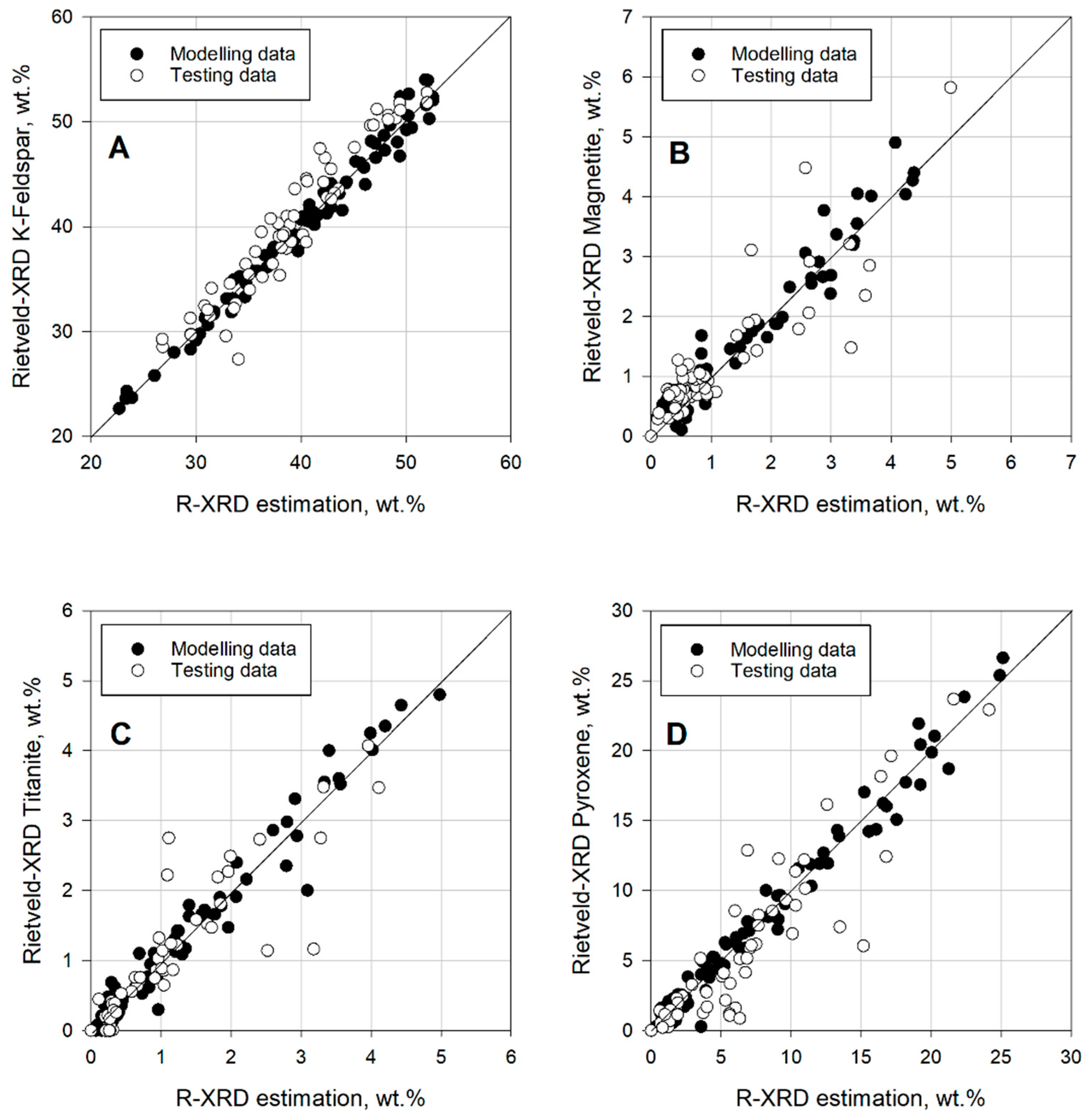
The EMC methods used showed an acceptable performance estimating abundant minerals, such as K-feldspar. The data points from K-feldspar were closer to the plot’s diagonal. Nonetheless, both methods failed to estimate correctly minerals with lower concentrations, such as titanite, magnetite, and pyroxene. Similar issues have been reported when estimating minerals in low concentration, see [16,23,39]. The problems when comparing to mineralogy, in this case are the accuracy of the XRD data and the way the estimation method behaves. For example, it is possible that certain measured elements estimated to be in a particular mineral actually belong to another mineral on the list, or even worse, to a mineral not considered at all. One example of estimation method could be the mineral titanite, which was consistently estimated incorrectly in the LS-XRD method. The cases of magnetite and pyroxene, both minerals in low quantity, also show errors with the same method. The R-XRD estimations showed better results estimating modal mineralogy than the LS-method. The trends are more consistent and closer to the diagonals on each plot. It is important to keep in mind that a method such as the R-XRD will produce regression results, which will look closer to the estimation during modelling. Moreover, the R-XRD method can be applied, and used to a defined bulk chemistry (e.g., specific lithology or concentrates). The R-XRD methodology might only be valid within restricted chemical populations, thus making the method suitable for its use at operational scale only by applying it to those chemical populations.

The obtained EMC estimations can be compared with the estimated modal mineralogy and bulk chemistry, after calculating it back from the modal mineralogy. When comparing bulk chemistry differences, the LS-XRD method yields better results than the R-XRD method. Although the results of the latter are closer to the original differences between measured sets, thus similar error between both XRF data and Rietveld mineralogy. Smaller bulk chemistry errors indicate better results towards known calibrated data i.e., XRF measurements. Nonetheless, closer results do not necessarily mean better results. There is a bias when attempting such a comparison. This bias can be the assumptions made during quantification (e.g., pre-defined mineral list) and estimation (e.g., restrictions used).

When comparing modal mineralogy differences, the R-XRD estimation showed better results. Again, this does not necessarily mean that the method itself is better. It is necessary to keep in mind that the modal mineralogy comparison is uncalibrated; the diffraction patterns acquired and quantified by the Rietveld method are standard-less. This means that regardless of the quantification method used, the true modal mineralogy of the sample will remain unknown because the sample analyzed is unknown. This is not an issue if the analyzed samples have a known mineral composition, which is the case with synthetic samples as shown by [42].

Normalizing mineral chemistries gave a more realistic idea of the mineral chemistry of the minerals present in the deposit. Normalization takes into consideration the atom-site distribution of the main atoms in the structure and its substitutions. Normalizing mineral chemistries refines the composition by adding or removing elements that otherwise would not be present in the mineral structures measured by EPMA (e.g., H₂O wt % or C wt %) and are required in EMC estimations.

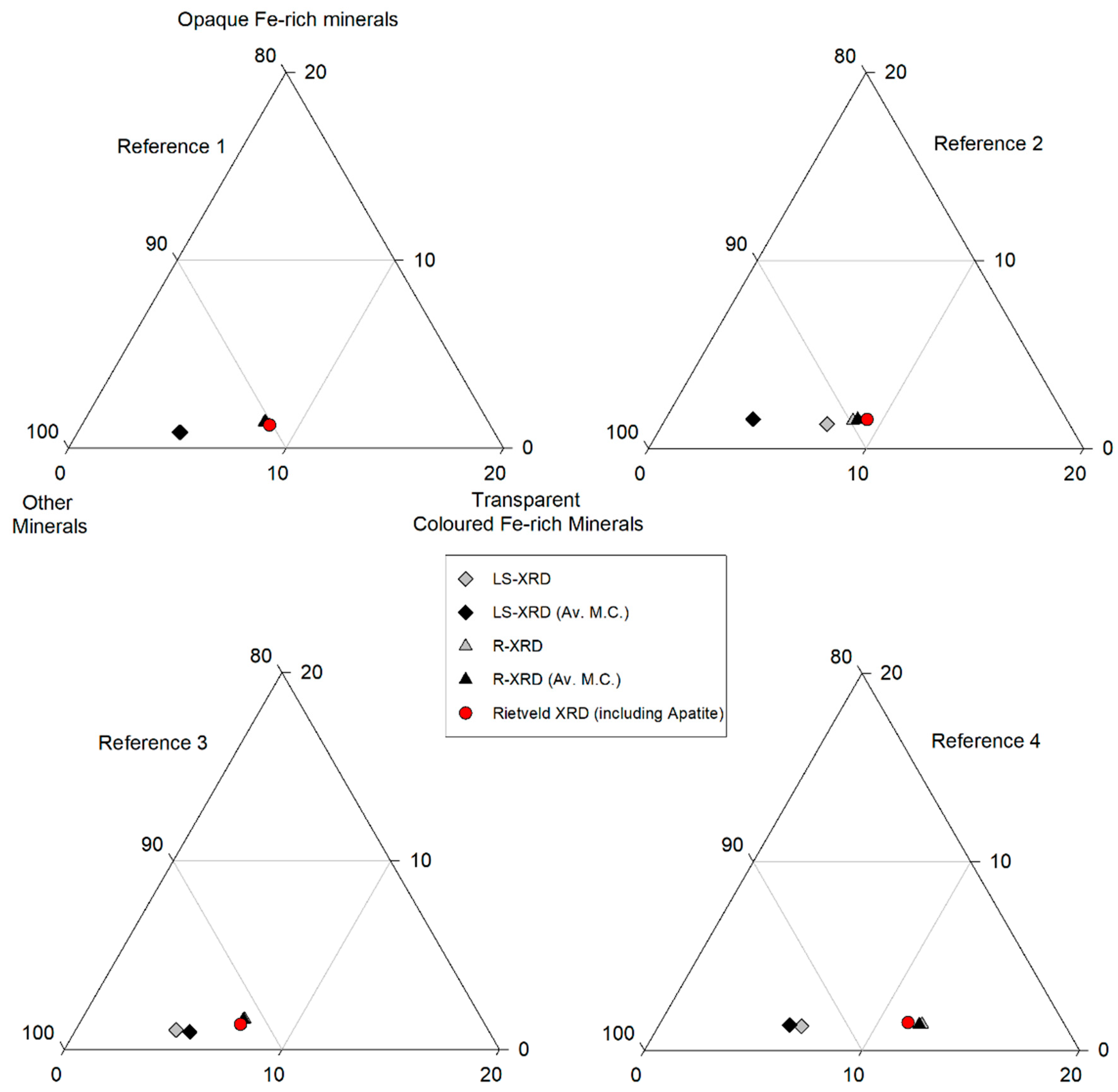
Mineral chemistry is not the main influence in EMC estimations. The use of different mineral chemistries showed no strong improvement on the mineralogical estimation. In Figure 7, the Reference 2 case showed an improvement when using mineral chemistry from that sample instead of the average mineral chemistry for the deposit in the LS-XRD estimation. Nonetheless, in all other cases, mineral chemistry did not show a significant change in mineralogical estimation.

The use of mineral chemistries from the minerals present in the deposit is necessary not only from a geological point of view, but also for processing and mineral estimations.

The use of average mineral chemistry values, obtained from different points in the deposit, for EMC estimations generally gave good results. The use of mineral chemistry leads to the idea of a new data layer to be included in mine planning and in a geometallurgical model: spatial mineral chemistry variations for the implementation of EMC estimations. Understanding and quantifying elemental variations of the minerals is not only useful geological information. Those mineral variations can be implemented in mine planning by quantification campaigns at the mine. Additionally, they can be used in estimating mineralogy for an improved mineralogical estimation that can be implemented as a routine at operational scale, thereby reducing uncertainties in a processing point-of-view.

The use of EMC method is a time efficient and low cost technique to estimate mineralogy based on bulk chemistry. It is time effective and low cost because virtually no extra analysis is required besides that needed to apply the methodology.

6. Conclusions

From the presented work the following conclusions can be drawn:

• Two element-to-mineral conversion (EMC) methodologies were applied for modal mineralogy estimation: the least square or LS-XRD and the regression or R-XRD methods. The R-XRD method showed better estimation results in terms of mineralogical performance with respect to Rietveld X-ray diffraction (XRD) data.
• The mineralogical estimation mainly depend method used. The use of a pre-defined mineral list for a Rietveld quantification routine, the use of data with a high detection limit such as XRD.
• Mineral chemistry did not significantly influence the mineral estimation.
• The mathematical method influenced the mineralogical estimation. The regression method shows accurate estimations, though this method is restricted to specific chemical conditions (e.g., lithology, concentrates, etc.).
• The R-XRD method is a regression method that shows potential for development, and can be implemented at operational scale for defined geochemical populations.
• The EMC methodologies are a geometallurgical tool that can be improved and eventually implemented in operations for their time efficiency and low cost associated.
• From a geometallurgical perspective, EMC is a good tool for increasing resource performance, easing decision-making processes, and reducing uncertainties.

References

1. Jeffrey, K. Characteristics of the Industrial Minerals Sector. In Industrial Minerals and Rocks, 7th ed.; Kogel, J.E., Trivedi, N.C., Barker, J.M., Krukowski, S.T., Eds.; Society for Mining, Metallurgy, and Exploration, Inc.: Englewood, CO, USA, 2006; pp. 3–6. [Google Scholar]
2. Jeffrey, K. Classification of Industrial Minerals and Rocks. In Industrial Minerals and Rocks, 7th ed.; Kogel, J.E., Trivedi, N.C., Barker, J.M., Krukowski, S.T., Eds.; Society for Mining, Metallurgy, and Exploration, Inc.: Englewood, CO, USA, 2006; pp. 7–11. [Google Scholar]
3. Harben, P.W. World Distribution of Industrial Minerals Deposits. In Industrial Minerals and Rocks, 7th ed.; Kogel, J.E., Trivedi, N.C., Barker, J.M., Krukowski, S.T., Eds.; Society for Mining, Metallurgy, and Exploration, Inc.: Englewood, CO, USA, 2006; pp. 13–48. [Google Scholar]
4. Boyd, R.; Gautneb, H. Mineral Resources in Norway: Potential and Strategic Importance, 2016 Update; Norges Geologiske Undersøkelse: Trondheim, Norway, 2016; p. 55.
5. Karlsen, T.; Sturt, B. Industrial minerals: Towards a future growth. Nor. Geol. Unders. 2000, 436, 7–14. [Google Scholar]
6. McLemore, V.T. Nepheline Syenite. In Industrial Minerals and Rocks, 7th ed.; Kogel, J.E., Trivedi, N.C., Barker, J.M., Krukowski, S.T., Eds.; Society for Mining, Metallurgy, and Exploration: Englewood, CO, USA, 2006; pp. 653–670. [Google Scholar]
7. Brown, T.; Idoine, N.; Raycraft, E.; Shaw, R.; Deady, E.; Hobbs, S.; Bide, T. World Mineral Production 2011–2015; British Geological Survey: Nottingham, UK, 2017.
8. Aasly, K.; Ellefmo, S. Geometallurgy applied to industrial minerals operations. Mineralproduksjon 2014, 5, 21–34. [Google Scholar]
9. Dominy, S.; O’Connor, L. Geometallurgy—Beyond conception. In Proceedings of the Geometallurgy 2016, Lima, Peru, 11–13 December 2016; pp. 3–10. [Google Scholar]
10. Dunham, S.; Vann, J.; Coward, S. Beyond Geometallurgy—Gaining Competitive Advantage by Exploiting the Broad View of Geometallurgy. Geomet 2011, 2011, 5–7. [Google Scholar]
11. Cropp, A.; Goodall, W.; Bradshaw, D.; Hunt, J.; Berry, R. Communicating and integrating geometallurgical data along the mining value chain. IMPC 2014, 2014, 1–12. [Google Scholar]
12. Hunt, J.A.; Berry, R.F. Geological Contributions to Geometallurgy: A Review. Geosci. Can. 2017, 44, 103–118. [Google Scholar] [CrossRef]
13. Lamberg, P. Particles—The Bridge between Geology and Metallurgy. In Proceedings of the Conference in Mineral Engineering, Luleå, Sweden, 8–9 February 2011; pp. 1–16. [Google Scholar]
14. Suazo, C.; Kracht, W.; Alruiz, O. Geometallurgical modelling of the Collahuasi flotation circuit. Miner. Eng. 2010, 23, 137–142. [Google Scholar] [CrossRef]
15. Rosa, D.; Rajavuori, L.; Korteniemi, J.; Wortley, M. Geometallurgical Modelling and Ore Tracking at Kittila Mine. In Advances in Applied Strategic Mine Planning; Springer: Cham, Switzerland, 2014; pp. 24–26. [Google Scholar]
16. Berry, R.; Hunt, J.; Parbhakar-Fox, A.; Lottermoser, B. Prediction of Acid Rock Drainage (ARD) from Calculated Mineralogy. In Proceedings of the 10th International Conference on Acid Rock Drainage and IMWA Annual Conference, Santiago, Chile, 21–24 April 2015; pp. 1–10. [Google Scholar]
17. Geis, H.P. Nepheline Syenite on Stjernøy, Northern Norway. Econ. Geol. 1979, 74, 1286–1295. [Google Scholar] [CrossRef]
18. Robins, B.; Often, M. The Seiland Igneous Province, North Norway. Field Trip Guidebook, IGCP Project 336; Norges Geologiske Undersøkelse (NGU): Finnmark, Norway, 1996; p. 34.
19. Heier, K.S. Layered gabbro, hornblendite, carbonatite and nepheline syenite on Stjernøy, North Norway. Nor. Geol. Tidsskr. 1961, 41, 155–190. [Google Scholar]
20. Li, X. Alkaline Magmatism, Water-Rock Interaction and Multiple Metamorphism in the Seiland Igneous Province, Northern Norway. Ph.D. Thesis, Albert-Ludwigs-Universität Freiburg, Freiburg, Germany, 2013. [Google Scholar]
21. Omotoso, O.; McCarty, D.K.; Hillier, S.; Kleeberg, R. Some successful approaches to quantitative mineral analysis as revealed by the 3rd Reynolds Cup contest. Clays Clay Miner. 2006, 54, 748–760. [Google Scholar] [CrossRef]
22. Benvie, B.; Chapman, N.M.; Robinson, D.J.; Kuhar, L.L. A robust statistical method for mineralogical analysis in geometallurgical diagnostic leaching. Miner. Eng. 2013, 52, 178–183. [Google Scholar] [CrossRef]
23. Parian, M.; Lamberg, P.; Möckel, R.; Rosenkranz, J. Analysis of mineral grades for geometallurgy: Combined element-to-mineral conversion and quantitative X-ray diffraction. Miner. Eng. 2015, 82, 25–35. [Google Scholar] [CrossRef]
24. O’Connor, B.; Chang, W.J. The amorphous character and particle size distributions of powders produced with the Micronizing Mill for quantitative X-ray powder diffractometry. X-ray Spectrom. 1986, 15, 267–270. [Google Scholar] [CrossRef]
25. Suortti, P.; Jennings, L. International Union of Crystallography Commission on Crystallographic Apparatus. Accuracy of structure factors from X-ray powder intensity measurements. Acta Crystallogr. Sect. A 1977, 33, 1012–1027. [Google Scholar] [CrossRef] [Green Version]
26. Røisi, I.; Aasly, K. The effect of graphite filler in sample preparation for automated mineralogy—A preliminary study. Mineralproduksjon 2018, 8, 1–23. [Google Scholar]
27. Kwitko-Ribeiro, R. New sample preparation developments to minimize mineral segregation in process mineralogy. In Proceedings of the 10th International Congress for Applied Mineralogy (ICAM); Springer: New York, NY, USA, 2012; pp. 411–417. [Google Scholar]
28. Bowen, N.L. Phase Equilibria Bearing on the Origin and Differentiation of Alkaline Rocks. 1945. Available online: http://earth.geology.yale.edu/~ajs/1945A/75.pdf (accessed on 26 May 2018).
29. Smith, J.V.; Brown, W.L. Intimate Feldspar Intergrowths. In Feldspar Minerals Volume 1: Crystal Structures, Physical, Chemical and Microtextural Properties; Springer-Verlag: Berlin, Germany, 1988; pp. 555–625. [Google Scholar]
30. Fandrich, R.; Gu, Y.; Burrows, D.; Moeller, K. Modern SEM-based mineral liberation analysis. Int. J. Miner. Proc. 2007, 84, 310–320. [Google Scholar] [CrossRef]
31. Kern, M.; Möckel, R.; Krause, J.; Teichmann, J.; Gutzmer, J. Calculating the deportment of a fine-grained and compositionally complex Sn skarn with a modified approach for automated mineralogy. Miner. Eng. 2018, 116, 213–225. [Google Scholar] [CrossRef]
32. Bryan, W.B.; Finger, L.T.; Chayes, F. Estimating proportions in petrographic mixing equations by least-squares approximation. Science 1969, 163, 926–927. [Google Scholar] [CrossRef] [PubMed]
33. Johnson, L.; Chu, C.; Hussey, G. Quantitative clay mineral analysis using simultaneous linear equations. Clays Clay Miner. 1985, 33, 107–117. [Google Scholar] [CrossRef]
34. Yvon, J.; Baudracco, J.; Cases, J.; Weiss, J. Eléments de minéralogie quantitative en micro-analyse des argiles. In Matériaux Argileux, Structure, Propriétés et Applications; Société Française de Minéralogie et Cristallographie: Paris, France, 1990; pp. 473–489. [Google Scholar]
35. Press, W.H.; Teukolsky, S.A.; Vetterling, W.T.; Flannery, B.P. Numerical Recipes—The Art of Scientific Computing, 3rd ed.; Cambridge University Press: Cambridge, UK, 2007. [Google Scholar]
36. Whiten, B. Calculation of mineral composition from chemical assays. Miner. Process. Extr. Metall. Rev. 2007, 29, 83–97. [Google Scholar] [CrossRef]
37. Barthelmy, D. Mineralogy Database, Webmineral. Available online: www.webmineral.com (accessed on 26 May 2018).
38. Deer, W.; Howie, R.; Zussman, J. An Introduction to the Rock-Forming Minerals, 3rd ed.; The Mineral Society: London, UK, 2013. [Google Scholar]
39. Berry, R.; Hunt, J.; McKnight, S. Estimating mineralogy in bulk samples. In Proceedings of the 1st International Geometallurgy Conference (GeoMet 2011), Brisbane, Australia, 5–7 September 2011; pp. 153–156. [Google Scholar]
40. Cheary, R.W.; Coelho, A. A Fundamental Parameters Approach To X-ray Line-Profile Fitting. J. Appl. Crystallogr. 1992, 25, 109–121. [Google Scholar] [CrossRef]
41. Deer, W.; Howie, R.; Zussman, J. Calculation of a chemical formula from a mineral analysis. In An Introduction to the Rock-Forming Minerals, 3rd ed.; The Mineral Society: London, UK, 2013; pp. 485–487. [Google Scholar]
42. Hestnes, K.; Sørensen, B. Evaluation of quantitative X-ray diffraction for possible use in the quality control of granitic pegmatite in mineral production. Miner. Eng. 2012, 39, 239–247. [Google Scholar] [CrossRef]
43. Lasdon, L.S.; Waren, A.D.; Jain, A.; Ratner, M. Design and testing of a generalized reduced gradient code for nonlinear programming. ACM Trans. Math. Softw. (TOMS) 1978, 4, 34–50. [Google Scholar] [CrossRef]
44. Hyndman, R.J.; Koehler, A.B. Another look at measures of forecast accuracy. Int. J. Forecast. 2006, 22, 679–688. [Google Scholar] [CrossRef] [Green Version]
45. Petruk, W. Applied Mineralogy in the Mining Industry, 1st ed.; Elsevier Science B.V.: Amsterdam, Switzerland, 2000. [Google Scholar]
Figure 1. Geological map of the Nabbaren nepheline syenite deposit located at the south side of the Stjernøy Island. The positions of drill-holes selected for sampling are shown as red dots. The samples selected for EPMA analyses are indicated by numbers and have a thicker central mark. Geological map modified from Geis [17].
Minerals 08 00325 g001
Figure 2. Average particle size distribution of the drill-holes. Based on 5 kg increment samples.
Minerals 08 00325 g002
Figure 3. Laboratory workflow. Arrow-shaped boxes represent processes, and square boxes represent the input and outputs obtained from the respective process.
Minerals 08 00325 g003
Figure 4. Typical aggregate of mafic minerals in the Nabbaren deposit. (A) Cluster of fine amphibole; and (B) mix cluster of amphibole and pyroxene. ne (nepheline), kfs (K-feldspar), amp (amphibole), px (pyroxene), cc (calcite), ttn (titanite), mt (magnetite), and po (pyrrhotite).
Minerals 08 00325 g004
Figure 5. Comparison between LS-XRD estimation (x-axis) and measured (y-axis) K-feldspar (A); magnetite (B); titanite (C); and pyroxene (D).
Minerals 08 00325 g005
Figure 6. Comparison between R-XRD estimations (x-axis) and measured (y-axis) K-feldspar (A); magnetite (B); titanite (C); and pyroxene (D).
Minerals 08 00325 g006
Figure 7. Modal mineralogy in wt % from the fraction −833/+74 µm. Different mineralogical estimations using averaged mineral chemistry from the deposit and the specific mineral chemistry for the georeferenced data. Av. M.C. = average mineral chemistry.
Minerals 08 00325 g007