Heap Leaching: Modelling and Forecasting Using CFD Technology


Abstract
1. Introduction
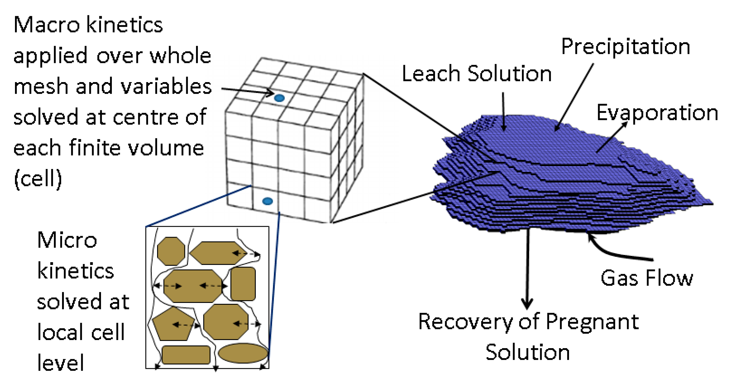
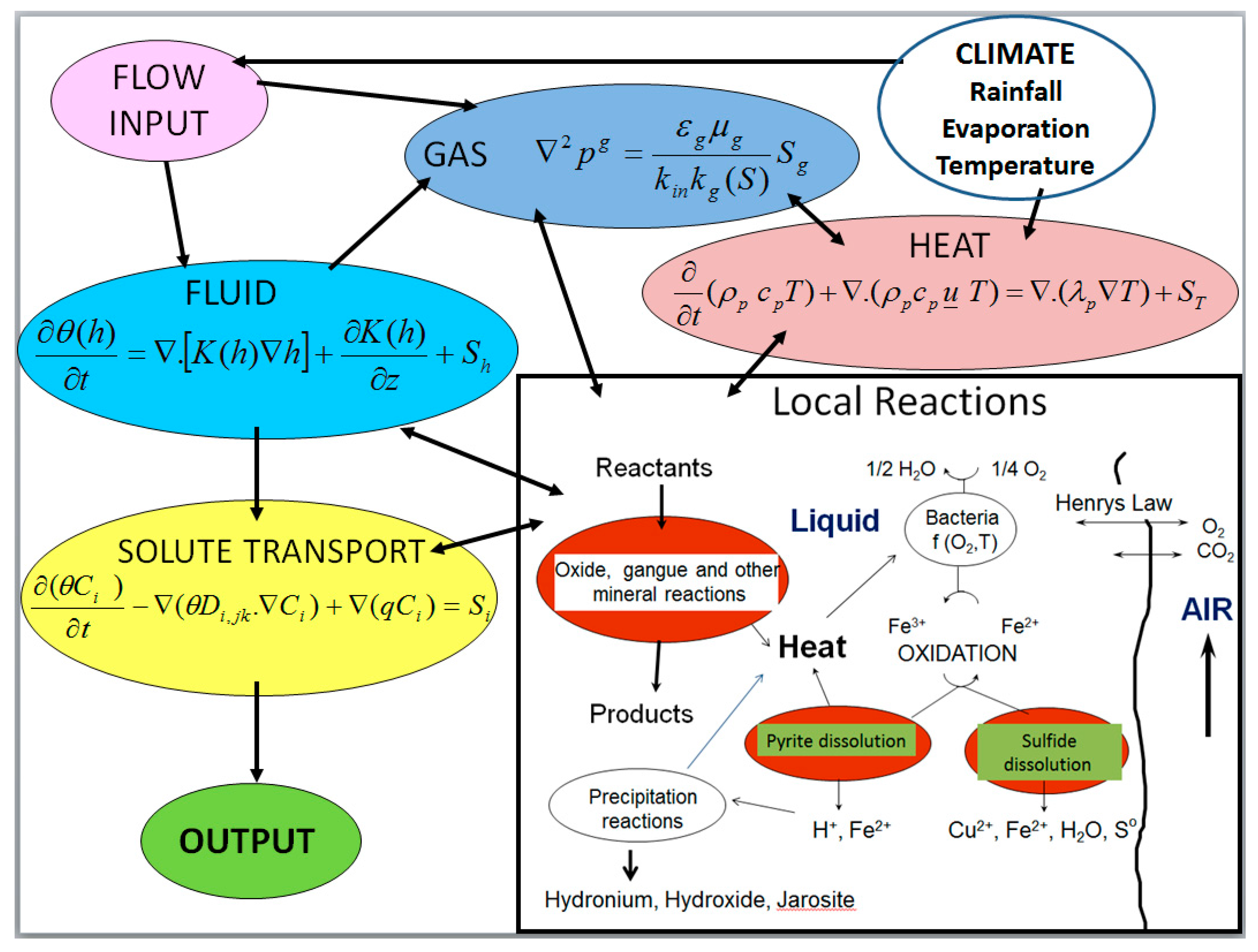
2. Computational Model
2.1. Liquid-Gas-Thermal Transport
2.2. Solid-Liquid-Gas Reactions
2.2.1. Solid-Liquid Dissolution
2.2.2. Gas-Liquid Oxygen Mass Transfer
2.2.3. Ferrous Oxidation
2.2.4. Liquid-Solid Precipitation
2.3. Leach Kinetics
2.3.1. Pyrite Rate Kinetics
2.3.2. Chalcopyrite Rate Kinetics
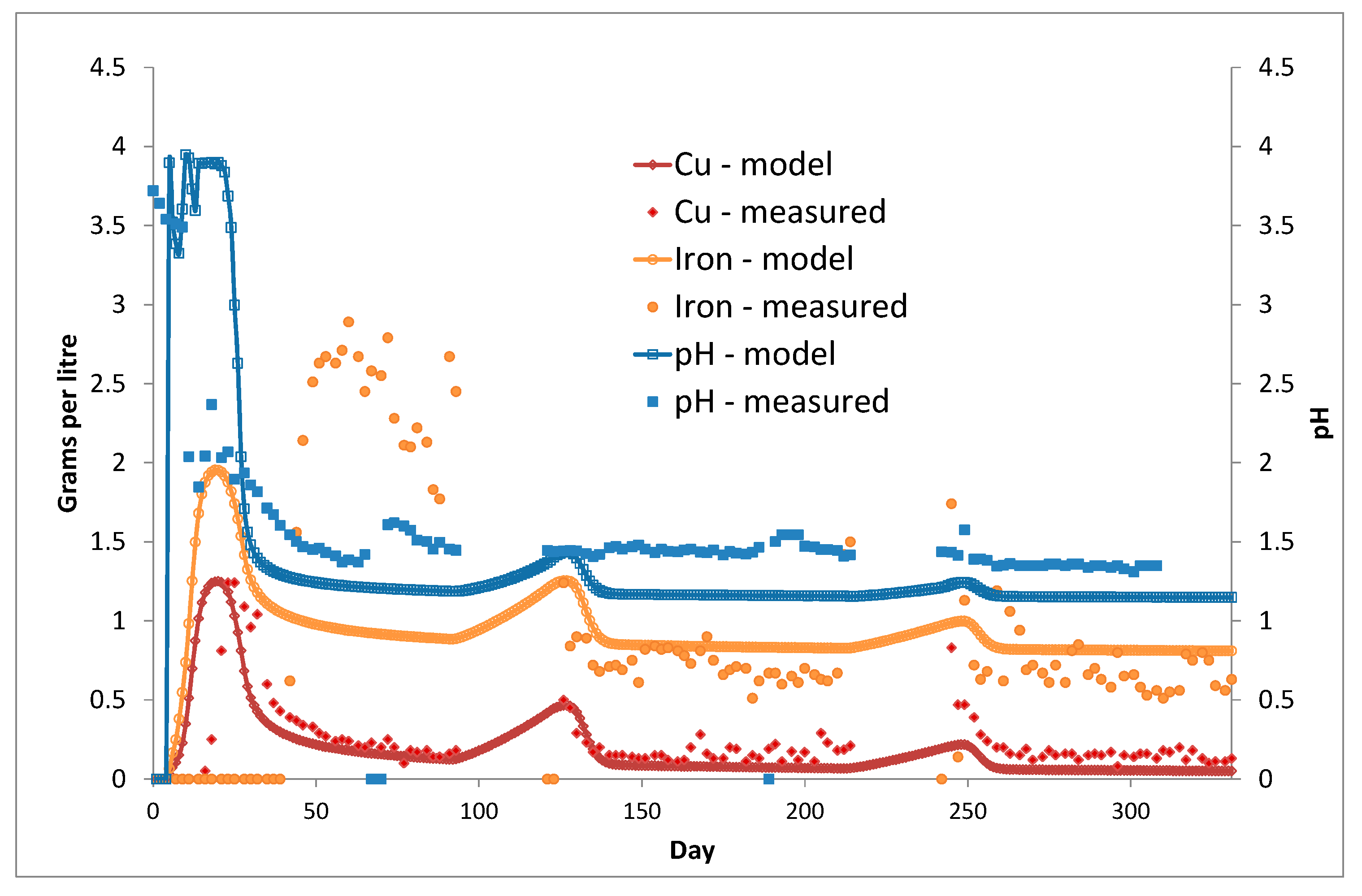
3. Column Leach Tests
Model Validation
4. Three-Dimensional ‘Virtual’ Chalcopyrite Stockpile
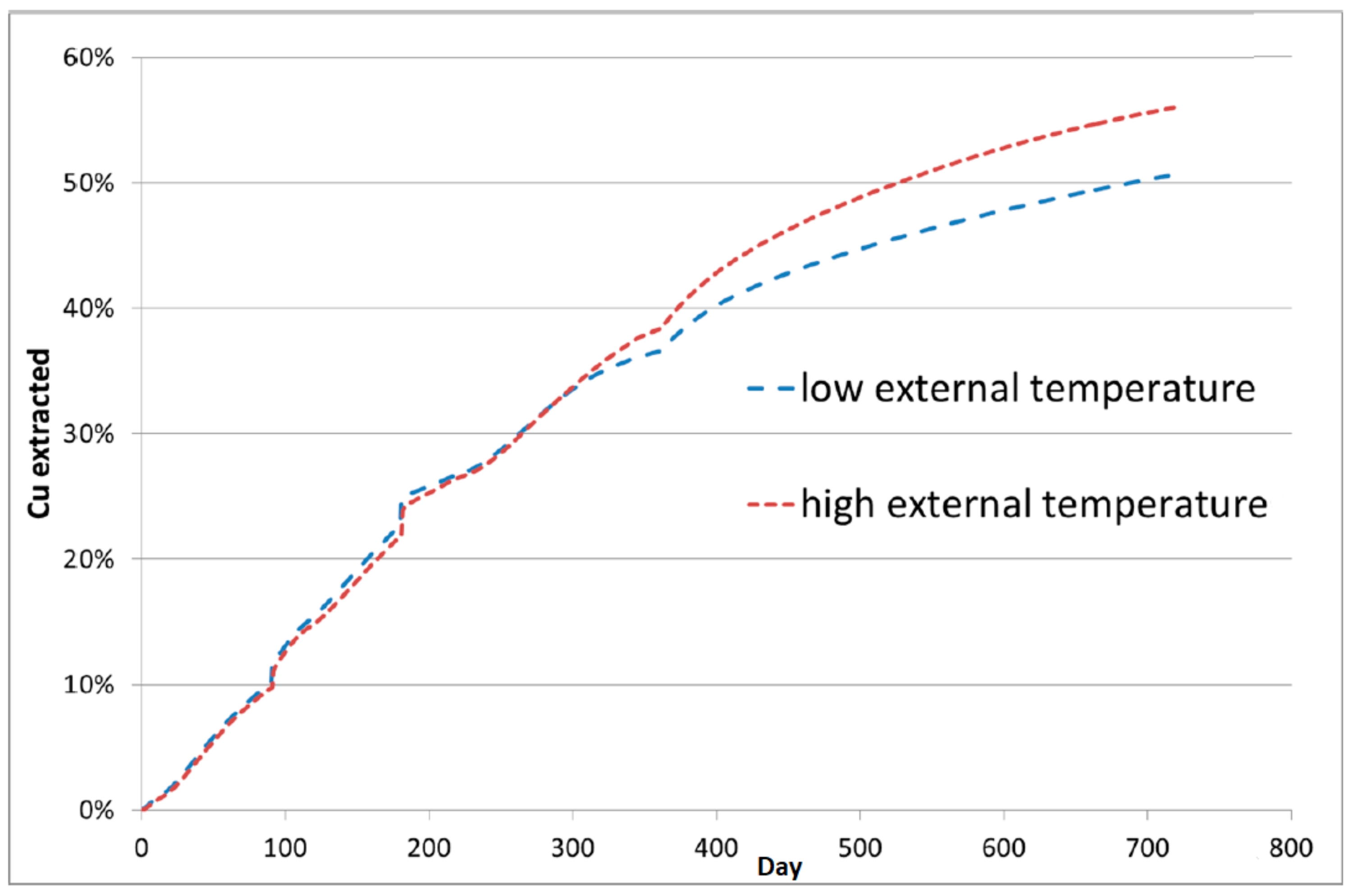
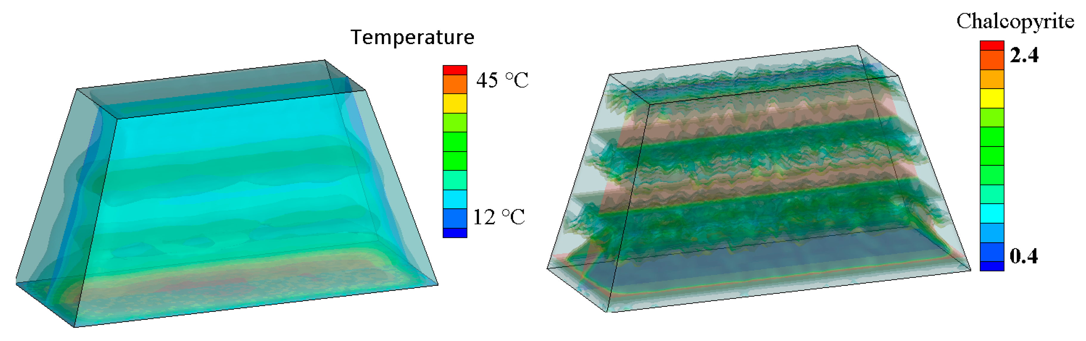
4.1. Thermal Effect on Recovery
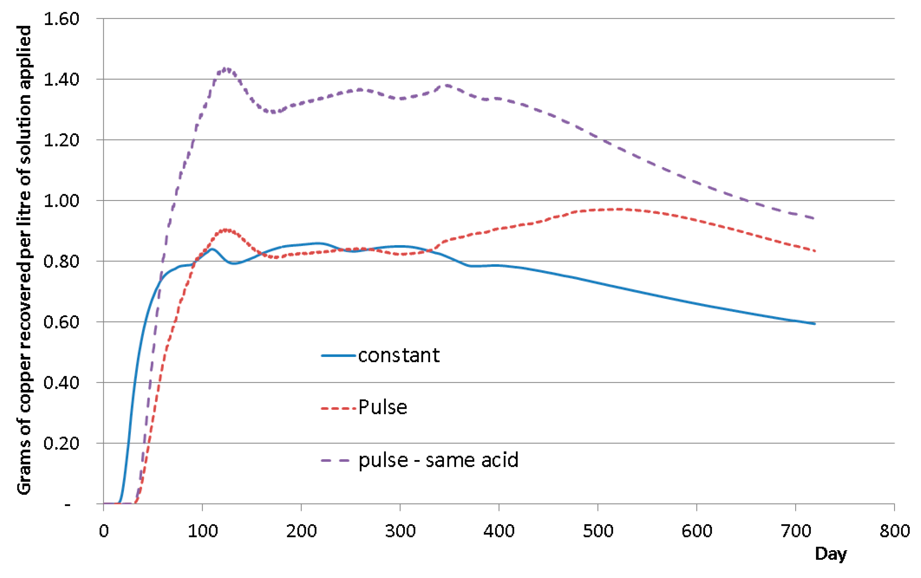
4.2. Continuous or Intermittent Leaching
5. Conclusions
Author Contributions
Conflicts of Interest
Nomenclature
| A | dimensionless | Experimentally calibrated mineral rate constant |
| B | dimensionless | Experimentally calibrated mineral rate constant |
| cj | J·kg−1·K−1 | Specific heat of phase j. |
| cp | J·kg−1·K−1 | Specific heat capacity of matrix |
| co | mol·m−3 | Concentration of available reactant at particle surface |
| Ci | mol·m−3 | Concentration of species i |
| D | m2·s−1 | Dispersion coefficient |
| Deff | m2·s−1 | Effective rock diffusion coefficient |
| e | Electronic charge | |
| h | m | Liquid pressure head |
| H | m | Total hydraulic head |
| kin | m | Intrinsic permeability |
| kg(S) | m·s−1 | The unsaturated permeability of gas at liquid saturation |
| K | m·s−1 | Hydraulic conductivity |
| KH | L·mol−1 | Henry’s law constant |
| Kc | dimensionless | Equilibrium constant |
| Mi | kg·mol−1 | Molecular weight of the mineral |
| mj | kg | Mass of phase j |
| mp | kg | Matrix mass |
| Oj | mol·L−1 | Oxygen in phase j |
| m | Gas pressure head | |
| q | m·s−1 | Darcy flux |
| ro | m | Initial particle radius |
| rm | m | Unreacted mineral radius |
| m | Mineral grain radius | |
| J·mol−1·K−1 | Universal gas constant | |
| , | dimensionless | Adjustable rate parameters |
| Sg | s−1 | Gas sink-source |
| Sh | s−1 | Liquid sink-source |
| s | Time | |
| S·m−1 | Electrical conductivity of the sulfur layer | |
| K | Temperature | |
| VFj | m3·m−3 | Volume fraction of phase j. |
| xi | kg·kg−1 | Mass fraction of the mineral |
| z | m·s−1 | Gravity direction |
| dimensionless | Apparent activity that is based on bulk species concentration | |
| dimensionless | Fraction of particle reacted | |
| kJ·mol−1 | Free energy of the system | |
| kJ·mol−1 | Enthalpy of reaction (constant) | |
| kJ·K−1·mol−1 | Entropy of reaction (constant) | |
| εg | m3·m−3 | Volume fraction of the gas phase |
| εp | m3·m−3 | Particle porosity |
| dimensionless | Shape factor for the mineral grain | |
| θ | m3·m−3 | Volume fraction of the liquid phase |
| λj | W·m−1·K−1 | Thermal conductivity of phase j. |
| λp | W·m−1·K−1 | Matrix thermal conductivity |
| μg | Kg·m−1·s−1 | Gas viscosity |
| kg·m−3 | Molar density | |
| kg·m−3 | Matrix density | |
| ρore | kg·m−3 | Ore density |
References
- Nesse, W.D. Introduction to Mineralogy; Oxford University Press: Oxford, UK, 2000. [Google Scholar]
- Bartlett, R.W. Solution Mining, 2nd ed.; Gordon & Breach Science Publishers: Amsterdam, The Netherlands, 1998. [Google Scholar]
- Petersen, J. Heap leaching as a key technology for recovery of values from low-grade ores—A brief overview. Hydrometallurgy 2016, 165, 206–212. [Google Scholar] [CrossRef]
- Ghorbani, Y.; Franzidis, J.-P.; Petersen, J. Heap Leaching Technology—Current State, Innovations, and Future Directions: A Review. Miner. Process. Extr. Metall. Rev. 2016, 37, 73–119. [Google Scholar] [CrossRef]
- Beven, K.; Germann, P. Macropores and water flow in soils revisited. Water Resour. Res. 2013, 49, 3071–3092. [Google Scholar] [CrossRef]
- Wu, A.X.; Yin, S.; Qin, W.; Liu, J.; Qiu, G. The effect of preferential flow on extraction and surface morphology of copper sulphides during heap leaching. Hydrometallurgy 2009, 95, 76–81. [Google Scholar] [CrossRef]
- Zhan, G.; Haggarty, S.; Ludwick, W. Hydrological Evaluation of Gold Leach Pad Rinsing. Mine Water Environ. 2012, 31, 307–311. [Google Scholar] [CrossRef]
- Van Staden, P.J.; Kolesnikov, A.V.; Petersen, J. Comparative assessment of heap leach production data—1. A procedure for deriving the batch leach curve. Miner. Eng. 2017, 101, 47–57. [Google Scholar] [CrossRef]
- Marsden, J.O.; Botz, M.M. Heap leach modeling—A review of approaches to metal production forecasting. Miner. Metall. Process. 2017, 34, 53–64. [Google Scholar] [CrossRef]
- Bouffard, S.C.; Dixon, D.G. Investigative Study into the hydrodynamics of heap leaching processes. Metall. Mater. Trans. B 2001, 32, 763–776. [Google Scholar] [CrossRef]
- Cariaga, E.; Concha, F.; Sepulveda, M. Flow through porous media with applications to heap leaching of copper ores. Chem. Eng. J. 2005, 111, 151–165. [Google Scholar] [CrossRef]
- De Andrade Lima, L.R.P. Liquid axial dispersion and holdup in column leaching. Miner. Eng. 2006, 19, 37–47. [Google Scholar] [CrossRef]
- Petersen, J.; Dixon, D.G. Modelling zinc heap bioleaching. Hydrometallurgy 2007, 85, 127–143. [Google Scholar] [CrossRef]
- Bouffard, S.C.; West-Sells, P.G. Hydrodynamic behaviour of heap leach piles: Influence of testing scale and material properties. Hydrometallurgy 2009, 98, 136–142. [Google Scholar] [CrossRef]
- Guzman, A.; Robertson, S.; Calienes, B. Constitutive relationships for the representation of a heap leach process. In Proceedings of the Heap Leach Solutions Conference, Vancouver, BC, Canada, 22–25 September 2013; van Zyl, D., Caldwell, J., Eds.; 2013; pp. 442–458. [Google Scholar]
- McBride, D.; Gebhardt, J.E.; Croft, T.N.; Cross, M. Modeling the hydrodynamics of heap leaching in sub-zero temperatures. Miner. Eng. 2016, 90, 77–88. [Google Scholar] [CrossRef]
- Bennett, C.R.; McBride, D.; Cross, M.; Gebhardt, J.E. A comprehensive model for copper sulphide heap leaching: Basic formulation and validation through column test simulation. Hydrometallurgy 2012, 127–128, 150–161. [Google Scholar] [CrossRef]
- Leahy, M.J.; Schwarz, M.P. Modelling jarosite precipitation in isothermal chalcopyrite bioleaching columns. Hydrometallurgy 2009, 98, 181–191. [Google Scholar] [CrossRef]
- Leahy, M.J.; Davidson, M.R.; Schwarz, M.P. A model for heap bioleaching of chalcocite with heat balance: Bacterial temperature dependence. Miner. Eng. 2005, 18, 1239–1252. [Google Scholar] [CrossRef]
- Leahy, M.J.; Schwarz, M.P.; Davidson, M.R. An air sparging CFD model of heap bioleaching of chalcocite. Appl. Math. Model. 2006, 30, 1428–1444. [Google Scholar] [CrossRef]
- Leahy, M.J.; Davidson, M.R.; Schwarz, M.P. A model for heap bioleaching of chalcocite with heat balance: Mesophiles and moderate thermophiles. Hydrometallurgy 2007, 85, 24–41. [Google Scholar] [CrossRef]
- Wu, A.; Liu, J.; Yin, S.; Wang, H. Analysis of coupled flow-reaction with heat transfer in heap bioleaching processes. Appl. Math. Mech. 2010, 3, 1473–1480. [Google Scholar] [CrossRef]
- Mostaghimi, P.; Tollit, B.S.; Neethling, S.J.; Gorman, G.J.; Pain, C. A control volume finite element method for adaptive mesh simulation of flow in heap leaching. J. Eng. Math. 2014, 87, 111–121. [Google Scholar] [CrossRef]
- Mostaghimi, P.; Percival, J.R.; Pavlidis, D.; Ferrier, R.J.; Gomes, J.L.M.A.; Gorman, G.J.; Jackson, M.D.; Neethling, S.J.; Pain, C. Anisotropic Mesh Adaptivity and Control Volume Finite Element Methods for Numerical Simulation of Multiphase Flow in Porous Media. Math. Geosci. 2015, 47, 417–440. [Google Scholar] [CrossRef]
- McBride, D.; Gebhardt, J.E.; Cross, M. A comprehensive oxide heap-leach model: Development and validation. Hydrometallurgy 2012, 113–114, 98–108. [Google Scholar] [CrossRef]
- McBride, D.; Cross, M.; Gebhardt, J.E. Heap leach modelling employing CFD technology: A ‘process’ heap model. Miner. Eng. 2012, 33, 72–79. [Google Scholar] [CrossRef]
- McBride, D.; Croft, T.N.; Cross, M.; Bennett, C.; Gebhard, J.E. Optimization of a CFD—Heap leach model and sensitivity analysis of process operation. Miner. Eng. 2014, 63, 57–64. [Google Scholar] [CrossRef]
- Miao, X.; Narsilio, G.A.; Wu, A.; Yang, B. A 3D dual pore-system leaching model. Part 1: Study on fluid flow. Hydrometallurgy 2017, 167, 173–182. [Google Scholar] [CrossRef]
- McBride, D.; llankoon, I.M.S.K.; Neethling, S.J.; Gebhardt, J.E.; Cross, M. Preferential flow behaviour in unsaturated packed beds and heaps: Incorporating into a CFD model. Hydrometallurgy 2017, 171, 402–411. [Google Scholar] [CrossRef]
- Ghorbani, Y.; Becker, M.; Petersen, J.; Morar, S.H.; Mainza, A.; Franzidis, J.-P. Use of X-ray computed tomography to investigate crack distribution and mineral dissemination in sphalerite ore particles. Miner. Eng. 2011, 24, 1249–1257. [Google Scholar] [CrossRef]
- Miller, G. Ore geotechnical effects on copper heap leach kinetics. In Proceedings of the 5th International Symposium Honoring Professor Ian M. Ritchie, Vancouver, BC, Canada, August 24–27 2003; TMS, 2003; pp. 329–342. [Google Scholar]
- Lin, Q.; Barker, D.J.; Dobson, K.J.; Lee, P.D.; Neethling, S.J. Modelling particle scale leach kinetics based on X-ray computed micro-tomography images. Hydrometallurgy 2016, 162, 25–36. [Google Scholar] [CrossRef]
- Ferrier, R.J.; Cai, L.; Lin, Q.; Gorman, G.J.; Neethling, S.J. Models for apparent reaction kinetics in heap leaching: A new semi-empirical approach and its comparison to shrinking core and other particle-scale models. Hydrometallurgy 2016, 166, 22–23. [Google Scholar] [CrossRef]
- Watling, H.R. The bioleaching of sulphide minerals with emphasis on copper sulphides—A review. Hydrometallurgy 2006, 84, 81–108. [Google Scholar] [CrossRef]
- Antonijevic, M.M.; Bogdanovic, G.D. Investigation of the leaching of chalcopyrite ore in acidic solutions. Hydrometallurgy 2004, 73, 245–256. [Google Scholar] [CrossRef]
- Córdoba, E.M.; Muñoz, J.A.; Blázquez, M.L.; González, F.; Ballester, A. Leaching of chalcopyrite with ferric ion. Part I: General aspects. Hydrometallurgy 2008, 93, 81–87. [Google Scholar] [CrossRef]
- Córdoba, E.M.; Muñoz, J.A.; Blázquez, M.L.; González, F.; Ballester, A. Passivation of chalcopyrite during its chemical leaching with ferric ion at 68 °C. Miner. Eng. 2009, 22, 229–235. [Google Scholar] [CrossRef]
- Pradhan, N.; Nathsarma, K.C.; Srinivasa Rao, K.; Sukla, L.B.; Mishra, B.K. Heap bioleaching of chalcopyrite: A review. Miner. Eng. 2008, 21, 355–365. [Google Scholar] [CrossRef]
- Nazari, G.; Asselin, E. Morphology of chalcopyrite leaching in acidic ferric sulfate media. Hydrometallurgy 2009, 96, 183–188. [Google Scholar] [CrossRef]
- Viramontes-Gamboa, G.; Peña-Gomar, M.M.; Dixon, D.G. Electrochemical hysteresis and bistability in chalcopyrite passivation. Hydrometallurgy 2010, 105, 140–147. [Google Scholar] [CrossRef]
- Kimball, B.E.; Rimstidt, J.D.; Brantley, S.L. Chalcopyrite dissolution rate laws. Appl. Geochem. 2010, 25, 972–983. [Google Scholar] [CrossRef]
- Li, Y.; Kawashima, N.; Li, J.; Chandra, A.P.; Gerson, A.R. A review of the structure, and fundamental mechanisums and kinetics of the leaching of chalcopyrite. Adv. Colloid Interface Sci. 2013, 197–198, 1–32. [Google Scholar] [PubMed]
- Buckley, A.N.; Woods, R. An X-ray photoelectron spectroscopic study of the oxidation of chalcopyrite. Aust. J. Chem. 1984, 37, 2403–2413. [Google Scholar] [CrossRef]
- Dutrizac, J.E. Elemental sulphur formation during the ferric sulphate leaching of chalcopyrite. Can. Metall. Q. 1989, 28, 337–344. [Google Scholar] [CrossRef]
- Hackl, R.P.; Dreisinger, D.B.; Peters, E.; King, J.A. Passivation of chalcopyrite during oxidative leaching in sulfate media. Hydrometallurgy 1995, 39, 25–48. [Google Scholar] [CrossRef]
- Harmer, S.L.; Thomas, J.E.; Fornasiero, D.; Gerson, A.R. The evolution of surface layers formed during chalcopyrite leaching. Geochim. Cosmochim. Acta 2006, 70, 4392–4402. [Google Scholar] [CrossRef]
- Stott, M.B.; Watling, H.R.; Franzmann, P.D.; Sutton, D. The role of iron-hydroxy precipitates in the passivation of chalcopyrite during bioleaching. Miner. Eng. 2000, 13, 1117–1127. [Google Scholar] [CrossRef]
- Tshilombo, A.F. Mechanism and Kinetics of Chalcopyrite Passivation and Depassivation during Ferric and Microbial Leaching. Ph.D. Thesis, University of British Columbia, Vancouver, BC, Canada, 2004. [Google Scholar]
- Dreisinger, D.; Abed, N. A fundamental study of the reductive leaching of chalcopyrite using metallic iron part I: Kinetic analysis. Hydrometallurgy 2002, 66, 37–57. [Google Scholar] [CrossRef]
- Brierley, J.A.; Brierley, C.L. Present and future commercial applications of biohydrometallurgy. Hydrometallurgy 2001, 59, 233–239. [Google Scholar] [CrossRef]
- Olsen, G.J.; Brierley, J.A.; Brierley, C.L. Bioleaching review part B: Progress in bioleaching: Applications of microbial processes by the minerals industries. Appl. Microbiol. Biotechnol. 2003, 63, 249–257. [Google Scholar] [CrossRef] [PubMed]
- Robertson, S.; Sayedbagheri, A.; Van Staden, P.; Guzman, A. Advances in heap leach research and development. In Proceedings of the ALTA 2010 Nickel-Cobalt-Copper Conference, Perth, Australia, 24–26 May 2010. [Google Scholar]
- Panda, S.; Sanjay, K.; Sukla, L.P.; Pradhan, N.; Subbaiah, T.; Mishra, B.K.; Prasad, M.S.R.; Ray, S.K. Insights into heap bioleaching of low grade chalcopyrite ores—A pilot scale study. Hydrometallurgy 2012, 125–126, 157–165. [Google Scholar] [CrossRef]
- Ekenes, J.M.; Caro, C.A. Improving leaching recovery of copper from low-grade chalcopyrite ores. Miner. Metall. Process. 2013, 30, 180–185. [Google Scholar]
- Rucker, D.F.; Zaebst, R.J.; Gillis, J.; Cain, J.C.; Teague, B. Drawing down the remaining copper inventory in a leach pad by way of subsurface leaching. Hydrometallurgy 2017, 169, 382–392. [Google Scholar] [CrossRef]
- Chen, B.-W.; Wen, J.-K. Feasibility study on heap bioleaching of chalcopyrite. Rare Met. 2013, 32, 524–531. [Google Scholar] [CrossRef]
- Panda, S.; Akcil, A.; Pradhan, N.; Deveci, H. Current scenario of chalcopyrite bioleaching: A review on the recent advances to its heap-leach technology. Bioresour. Technol. 2015, 196, 694–706. [Google Scholar] [CrossRef] [PubMed]
- Petersen, J. Modelling of bioleach processes: Connection between science and engineering. Hydrometallurgy 2010, 104, 404–409. [Google Scholar] [CrossRef]
- Gebhardt, J.E.; Gilbert, S.R.; McBride, D.; Cross, M.; Bennett, C. Chalcopyrite leach kinetics described within a comprehensive CFD heap leach model. In Proceedings of the International Minerals Processing Congress (IMPC 2014), Santiago, Chile, 20–24 October 2014. [Google Scholar]
- Croft, N.; Pericleous, K.A.; Cross, M. PHYSICA: A multiphysics environment for complex flow processes. In Numerical Methods in Laminar and Turbulent Flow; Taylor, C., Durbetaki, P., Eds.; Pineridge Press: Swansea, UK, 1995; Volume 95, pp. 1269–1280. [Google Scholar]
- McBride, D.; Cross, M.; Croft, T.N.; Bennett, C.R.; Gebhardt, J.E. Computational modelling of variably saturated flow in porous media with complex three-dimensional geometries. Int. J. Numer. Methods Fluids 2006, 50, 1085–1117. [Google Scholar] [CrossRef]
- Paul, B.C.; Sohn, H.Y.; McCarter, M.K. Model for Ferric Sulfate Leaching of Copper Ores Containing a Variety of Sulfide Minerals: Part I: Modeling Uniform Size Ore Fragments. Metall. Trans. B 1992, 23B, 537–548. [Google Scholar] [CrossRef]
- Garrels, R.M.; Christ, C.L. Solutions, Minerals, and Equilibria; Freeman, Cooper & Company: San Francisco, CA, USA, 1965. [Google Scholar]
- Stumm, W.; Morgan, J.J. Aquatic Chemistry: An Introduction Emphasizing Chemical Equilibria in Natural Waters; Wiley-Interscience: New York, NY, USA, 1970. [Google Scholar]
- Munoz-Castillo, P.B. Reaction Mechanisms in the Acid Ferric Sulfate Leaching of Chalcopyrite. Ph.D. Thesis, University of Utah, Salt Lake City, UT, USA, 1977. [Google Scholar]
- Munoz, P.B.; Miller, J.D.; Wadsworth, M.E. Reaction Mechanism for the Acid Ferric Sulfate Leaching of Chalcopyrite. Metall. Trans. B 1979, 10B, 149–158. [Google Scholar] [CrossRef]
- Kaplun, K.; Li, J.; Kawashima, N.; Gerson, A.R. Cu and Fe chalcopyrite leach activation energies and the effect of added Fe3+. Geochim. Cosmochim. Acta 2011, 75, 5865–5878. [Google Scholar] [CrossRef]
- Tuller, W.N. The Sulfur Data Book; McGraw-Hill Book Company, Inc.: New York, NY, USA, 1954; p. 59. [Google Scholar]
- Bouffard, S.C. Agglomeration for heap leaching: Equipment design, agglomerate quality control, and impact on the heap leach process. Miner. Eng. 2008, 21, 1115–1125. [Google Scholar] [CrossRef]


| Model Level | 1 | 2 | 3 | 4 | 5 | 6 |
|---|---|---|---|---|---|---|
| Model Type | Spreadsheet No scale-up | Spreadsheet with scale-up | Spreadsheet scale-up and inventory adjustment | Mass-balance software | Fluid flow + chemical reactions | Comprehensive CFD ‘virtual 3D heap’ |
| Tonnes & grade of ore over time | ✓ | ✓ | ✓ | ✓ | ✓ | ✓ |
| Column leach data utilised | ✓ Extraction curve | ✓ With delay factor | ✓ + scale-up factor | ✓ + scale-up factor | ✓ calibrate leach kinetics | ✓ to calibrate leach kinetics |
| Solution inventory tracked | ✓ | ✓ | ✓ | ✓ | ✓ | |
| Heap permeability | Scale-up factor | Scale-up factor | ✓ dynamic by ore type | ✓ dynamically, local, depth & time | ||
| Gas-liquid flow | ✓ | ✓ | ✓ | |||
| Solution channelling | Discount factor | Discount factor | ✓ | ✓ | ||
| Oxidation | ✓ | ✓ | ||||
| Particle kinetics | ✓ | ✓ | ||||
| Thermodynamics | ✓ reactions | ✓ + liquid-solid-gas | ||||
| Bacteria | ✓ | ✓ | ||||
| Gangue reactions | ✓ | |||||
| Precipitation | ✓ | |||||
| Meteorological rain, evaporation, temperature | ✓ | ✓ + internal liquid freezing |
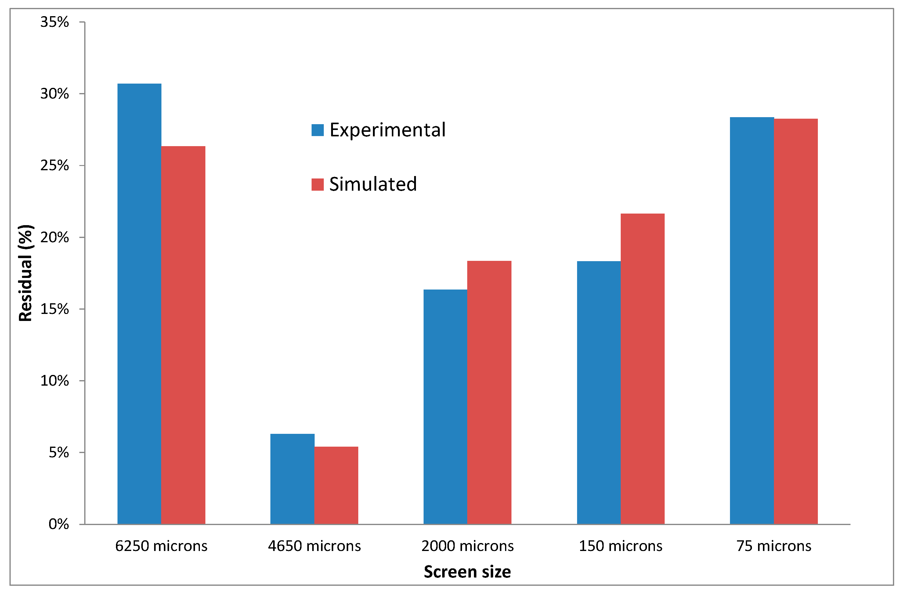
| Mesh Size (Microns) | % Weight | % Cu |
|---|---|---|
| 6250 | 36.4 | 0.22 |
| 4750 | 7.5 | 0.22 |
| 2000 | 21.3 | 0.2 |
| 150 | 23.9 | 0.2 |
| 75 | 10.9 | 0.68 |
| Average | 0.26 |
© 2018 by the authors. Licensee MDPI, Basel, Switzerland. This article is an open access article distributed under the terms and conditions of the Creative Commons Attribution (CC BY) license (http://creativecommons.org/licenses/by/4.0/).
Share and Cite
McBride, D.; Gebhardt, J.; Croft, N.; Cross, M. Heap Leaching: Modelling and Forecasting Using CFD Technology. Minerals 2018, 8, 9. https://doi.org/10.3390/min8010009
McBride D, Gebhardt J, Croft N, Cross M. Heap Leaching: Modelling and Forecasting Using CFD Technology. Minerals. 2018; 8(1):9. https://doi.org/10.3390/min8010009
Chicago/Turabian StyleMcBride, Diane, James Gebhardt, Nick Croft, and Mark Cross. 2018. "Heap Leaching: Modelling and Forecasting Using CFD Technology" Minerals 8, no. 1: 9. https://doi.org/10.3390/min8010009
APA StyleMcBride, D., Gebhardt, J., Croft, N., & Cross, M. (2018). Heap Leaching: Modelling and Forecasting Using CFD Technology. Minerals, 8(1), 9. https://doi.org/10.3390/min8010009