Relating Topological and Electrical Properties of Fractured Porous Media: Insights into the Characterization of Rock Fracturing

Abstract

Numerous laboratory and field experiments suggest that electrical properties of fractured rocks may provide critical information regarding the topological properties of the underlying fracture networks. However, a lack of numerical studies dedicated to realistic fractured media prevents us from assessing, in a systematic manner, the relationships between electrical and topological properties in complex domains for which a representative elementary volume may not exist. To address this issue, we conduct an extended numerical analysis over a large range of realistic fractured porous media with an explicit description of the fractures that takes into account the fracture–matrix interactions. Our work shows that the fracture density determines the suitability of Archie’s law for describing effective electrical properties with complex behavior associated with small fracture densities. In particular, for fracture networks at the percolation threshold surrounded by a low-porosity matrix, the effective petrophysical relationships are impacted by the assumed fracture-length distribution and the exchange of electric current between the fractures and surrounding matrix. These results help in understanding experimental observations that were difficult to explain so far, suggesting that the effective electrical properties of fractured rock may be used to obtain insights into the properties of their geological structures.

1. Introduction

Evaluating subsurface rock properties is a critical challenge in a wide variety of research fields and applications including hydrogeology, geothermal energy, natural resource prospecting and the long-term storage of toxic waste (e.g., [1,2,3]). In the case of fractured rocks, the main challenge is to identify the presence of fractures and estimate their properties, as these highly permeable structures play a key role in the natural environment (e.g., [4,5,6]). For the extraction of water, hydrocarbons or heat, fractures can help to access the resource stored in the matrix. With regard to assessing the risk of contaminant migration, they can quickly propagate pollutants that are spread on the surface (e.g., agricultural or industrial chemicals) or stored in deep reservoirs (e.g., radioelements or dissolved CO${}_2$).

Given the importance of fractures in various challenging environmental issues, a wide range of studies have been devoted to gathering information on these geological structures and determining how they are distributed and connected (e.g., [7,8,9]). In this regard, geophysical methods can give information that is complementary to traditional characterization techniques such as direct observation of fractures, pumping tests and tracer experiments (e.g., [10,11,12]). Among the numerous existing geophysical approaches, electrical resistivity measurements are of particular interest because the effective electrical properties that they provide are sensitive to fluid content and can be obtained over a wide range of spatial scales. These methods are used to infer rock porosity from in-situ measurements relying on laboratory-scale petrophysical relationships (e.g., [13,14,15]), but also to obtain vertically distributed information on reservoir content and heterogeneities along boreholes (e.g., [16,17,18]). As demonstrated by several studies, when electrical measurements are acquired along the Earth’s surface with various electrode spacing, they also provide information on the presence and properties of fractures at several depths (e.g., [19,20,21]).

Extracting the maximum amount of information from electrical resistivity measurements about the underlying geological structures requires a deep understanding of the link between topological and electrical properties. This has been the objective of numerous laboratory experiments (e.g., [22,23,24,25]) and modeling approaches (e.g., [26,27,28,29,30]) conducted for a wide variety of porous and fractured rocks. Whereas these studies defined and characterized the corresponding petrophysical relationships for porous media (e.g., [16,31,32]), some experimental results obtained for fractured-rock samples remain unexplained because the impact of the fracture-network properties on the resistivity response is unclear (e.g., [25,33,34,35]). From a numerical modeling standpoint, multiple-porosity model formulations show how the presence of vugs and fractures impacts the effective electrical properties of rocks (e.g., [14,26,36]). However, these formulations are based on either simplified fracture-network configurations, which are not representative of realistic field conditions, or effective medium theories, which assume that the fractured medium can be treated as a representative elementary volume (REV). Consequently, they are not adapted to heterogeneous and realistic fracture networks for which the existence of a REV is questionable (e.g., [37,38,39]). This limitation poses severe problems for acquiring a deep understanding of the effective electrical properties of fractured rocks and of the impact of their heterogeneity on these properties.

In this paper, we address the above shortcoming by improving our knowledge of the effective electrical properties of fractured rocks and by evaluating the impact of their structural heterogeneities on these properties. To this end, we conduct a systematic numerical analysis over a large range of fractured media, which are characterized by a complex and realistic organization of their structures (e.g., [8,39,40]). We use a recently developed modeling approach which is especially designed for modeling electrical current flow in complex and heterogeneous fractured rocks, and we demonstrate that (i) the fracture length distribution and fracture density have a significant impact on the relationships between the electrical properties and porosity of the considered systems; (ii) these properties are related by Archie’s law for large values of the fracture density; and (iii) for small values of this density, complex behaviors of these properties are observed and can be linked to some unexplained experimental results. In particular, considering fracture networks at the percolation threshold embedded into a low-porosity matrix results in fracture–matrix systems whose electrical properties are strongly impacted by the range of the considered fracture lengths, the spatial distribution of the fractures, as well as the exchanges of electric current between the fractures and surrounding matrix.

2. Methodological Background

2.1. Electrical Parameters

Defining the link between topological and electrical properties of rock samples is generally done by studying several electrical parameters and by analyzing how these parameters depend on the sample porosity. Considering a fully-saturated rock having electrical conductivity $\sigma$, for which the surface conductivity is negligible in comparison with the fluid conductivity ${\sigma }_w$, the impact of the topological properties on the electrical conductivity can be characterized by the electrical formation factor $F={\sigma }_w/\sigma$. This parameter is often related to the system porosity $\varphi$ using the empirical Archie’s law $F={\varphi }^{-m}$[16], where the Archie exponent (or cementation factor) m is close to 2 for granular porosity and around 1 for fissural-type porosity (e.g., [41]). In the latter case with low-porosity rocks, the relationship $F=\tau /\varphi$, where $\tau$ is defined as the electrical tortuosity, is also used (e.g., [17,42,43]), and corresponds to a particular case of the extended Archie’s law $F=a{\varphi }^{-m}$ (e.g., [44,45]) with geometric constant $a=\tau$ and $m=1$. As the electrical parameters m and $\tau$ provide meaningful and complementary information on the considered systems, they are used to characterize the topological properties of the fractured rock samples, sometimes independently of the relationship between F and $\varphi$ (e.g., [22,25,33,34,35,46]). More precisely, m is related to the pore geometry of the system and characterizes how the electric current samples the interconnected porosity (e.g., [22,29]), whereas $\tau$ is related to the irregularity of the electrical flow pathway and characterizes the complexity of this path through the system (e.g., [22,42,47]).

In the present study, we want to analyze how the electrical parameters F, m and $\tau$ depend on the porosity $\varphi$, the fracture network properties, and the fracture–matrix exchanges over a large range of low-porosity fractured rocks. To this end, we evaluate these parameters using the numerical approach and simulations described below considering the following definitions (e.g., [16,48,49]):

$$\begin{array}{c}\hfill F={\sigma }_w/\sigma ,m=-logF/log\varphi ,\tau =F\varphi .\end{array}$$

(1)

2.2. Modeling Approach

We wish to evaluate the electrical parameters in (1) for complex and heterogeneous fractured-rock formations characterized by a significant contrast between the electrical conductivity of the fractures and that of the surrounding matrix, and for which the electrical properties cannot be homogenized. To this end, we use the discrete-dual-porosity (DDP) approach proposed by [50], which is based on an explicit representation of the fractures and takes into account the electric current exchanged between these fractures and the surrounding matrix.

This method is used to solve numerically the boundary-value problem

$$\begin{array}{cc}\hfill -\nabla ·({\sigma }_{\mathbf{x}}\nabla {\mathsf{\Phi }}_{\mathbf{x}})=0,& \mathbf{x}\in \mathsf{\Omega }\hfill \end{array}$$

(2a)

$$\begin{array}{cc}\hfill {\mathsf{\Phi }}_{\mathbf{x}}={\mathsf{\Phi }}_i^{\ast },& \mathbf{x}\in {\Gamma }_i\mathrm{with}i=0,1\hfill \end{array}$$

(2b)

$$\begin{array}{cc}\hfill {\sigma }_{\mathbf{x}}\frac{\partial {\mathsf{\Phi }}_{\mathbf{x}}}{\partial n}=0,& \mathbf{x}\in {\Gamma }_i\mathrm{with}i=2,3,\hfill \end{array}$$

(2c)

where ${\sigma }_{\mathbf{x}}\left(\mathbf{x}\right)$ and ${\mathsf{\Phi }}_{\mathbf{x}}\left(\mathbf{x}\right)$ are the electrical conductivity and electric potential, respectively, in the two-dimensional square domain $\mathsf{\Omega }$ surrounded by the left, right, top and bottom borders ${\Gamma }_0$, ${\Gamma }_1$, ${\Gamma }_2$ and ${\Gamma }_3$, respectively. Setting the Dirichlet conditions ${\mathsf{\Phi }}_0^{\ast }$ and ${\mathsf{\Phi }}_1^{\ast }$ to 1 V and 0 V, respectively, implies that the effective electrical conductivity in one direction can be defined as $\sigma =J_1$ with $J_1$ the electric flux leaving the right side of the domain. This definition is consistent with laboratory experiments that have been conducted on rock samples (e.g., [25,33,34,35]), and the reader should refer to [50] for a numerical multi-directional evaluation of $\sigma$. Note that, in this work, our DDP approach is always used with 21 grid-cells in each direction and that the numerical convergence of these results has been verified through tests using a finer discretization.

2.3. Numerical Simulations

In order to study complex and heterogeneous fractured-rock formations, we consider unit square domains of size $L=1$ m consisting of random distributions of fractures having positions and orientations drawn from a uniform distribution. The lengths of these fractures are defined from either a uniform distribution ranging from $L_{min}$ to $L_{max}$ or a power-law distribution parametrized by the minimum fracture length $L_{min}$ and power law exponent a. The fracture density is characterized by the percolation parameter $p={\sum }_i^{N_f}{l}_i^2/L^2$, where $N_f$ is the number of fractures and $l_i$ is the length of each fracture i [51]. The final fractured porous domains are composed of the surrounding matrix and the interconnected fracture network, which is defined as the network of fractures that connect the left and right sides of the domains. Note that if there are no fractures connecting the left and right sides of the domains, the overall electrical conductivity is defined by the matrix conductivity.

For this study, we generated fracture networks by setting $L_{min}$ to ${10}^{-2}$ m and $L_{max}$ to 1, 0.5, 0.2, 0.1 and 0.05 m for the uniformly-distributed fracture lengths, and a to 1.5, 2, 2.5, 3 and 3.5 for the power-law-distributed fracture lengths. Figure 1 shows examples of the corresponding interconnected fracture networks for $p=6$, 12 and 18. In our simulations, the fracture aperture $b_f$ is set to ${10}^{-4}$ m, the electrical conductivity of the fractures is set to the fluid conductivity ${\sigma }_w=1$ S/m, and the matrix electrical conductivity is determined using Archie’s law ${\sigma }_b={\sigma }_w{\varphi }_b^{m_b}$ with the low matrix (or bulk rock) porosity ${\varphi }_b=0.5\%$ and the matrix Archie exponent $m_b=2$, resulting in ${\sigma }_b=2.5\times {10}^{-5}$ S/m [34].

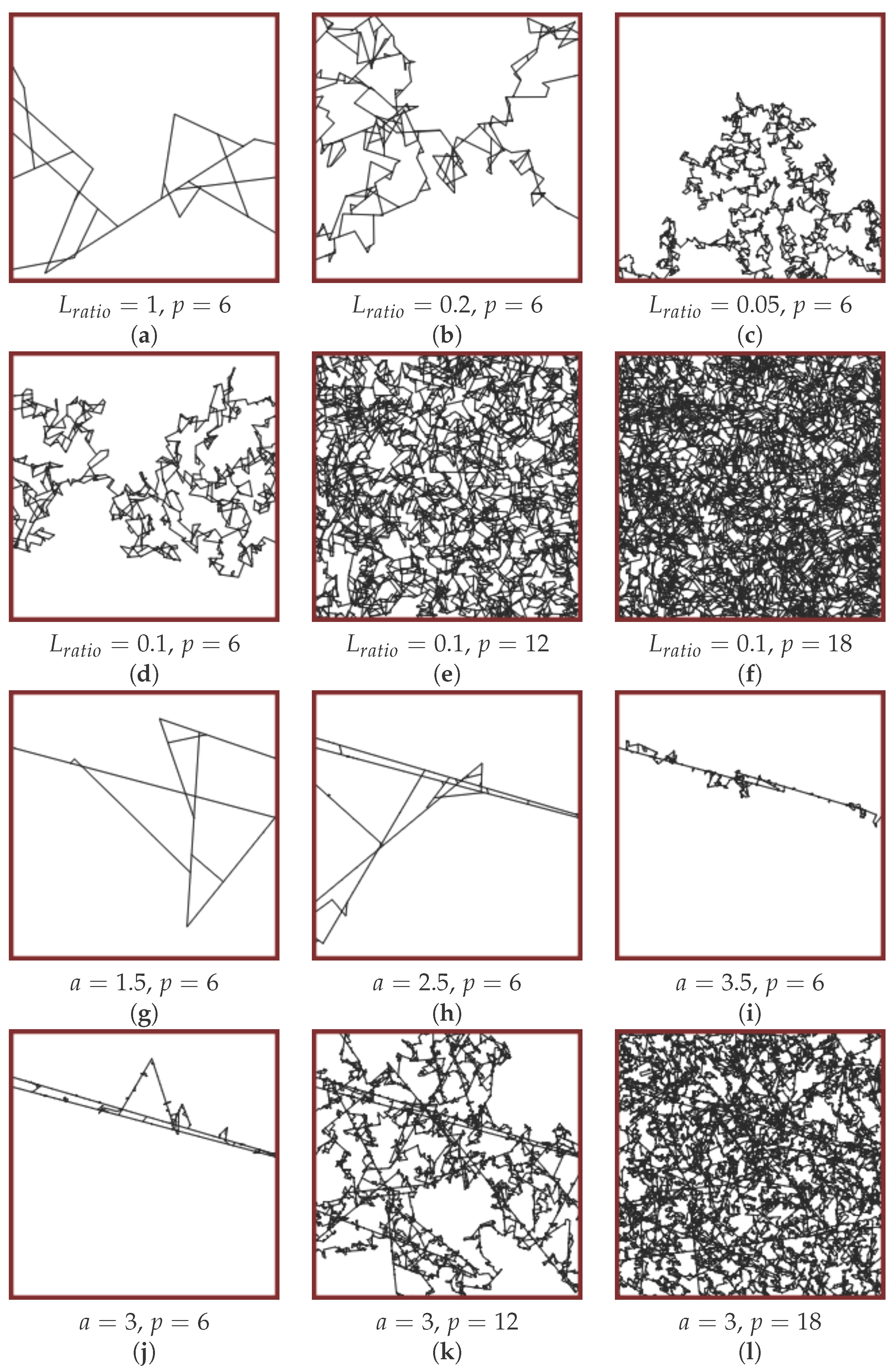
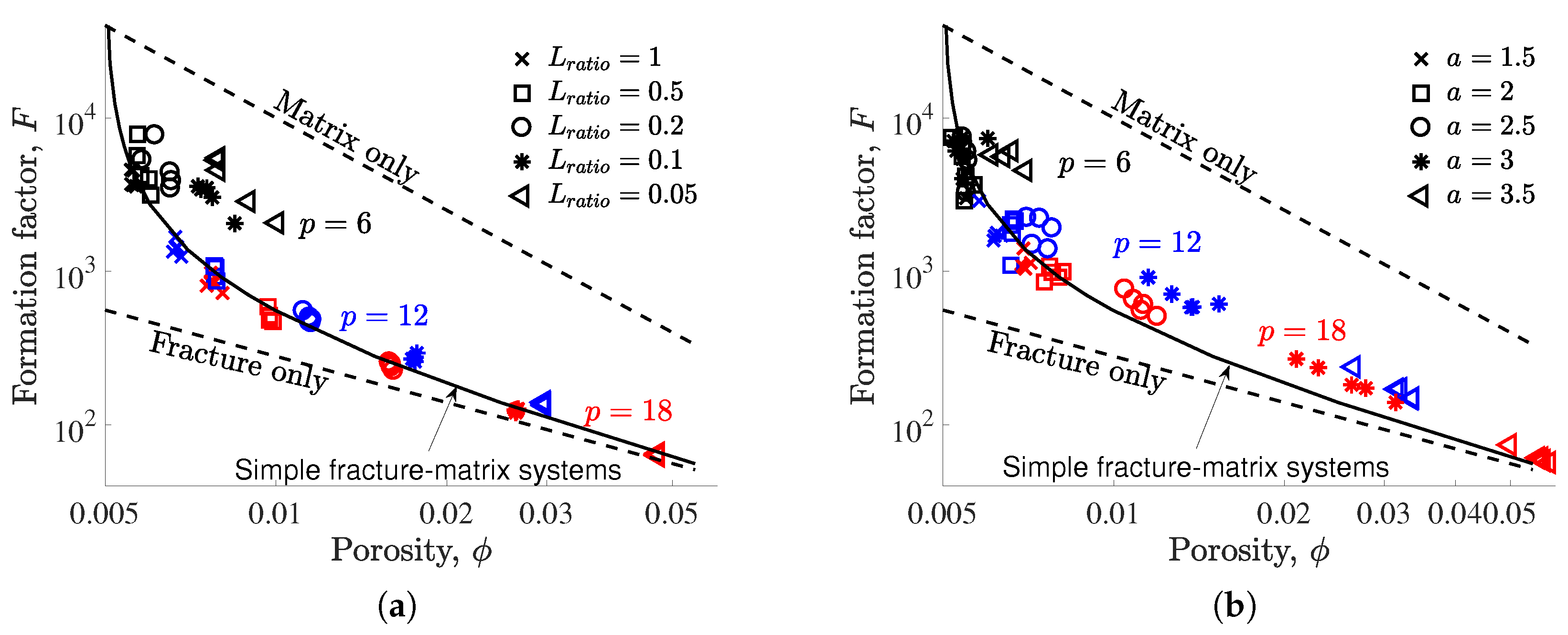
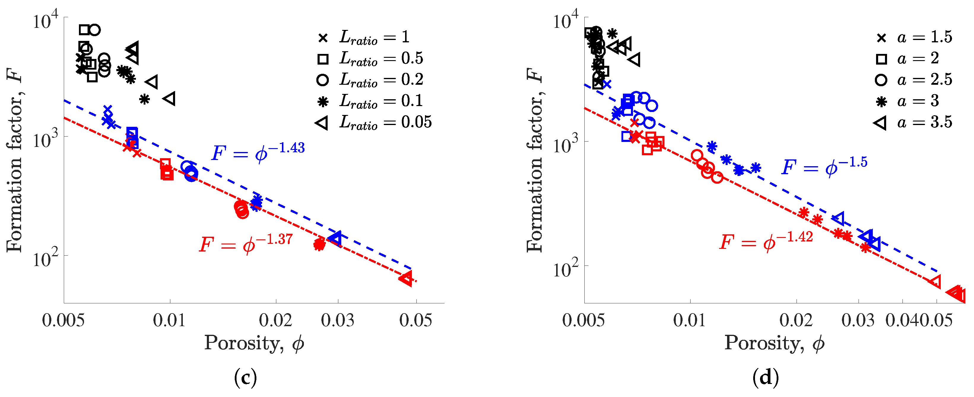
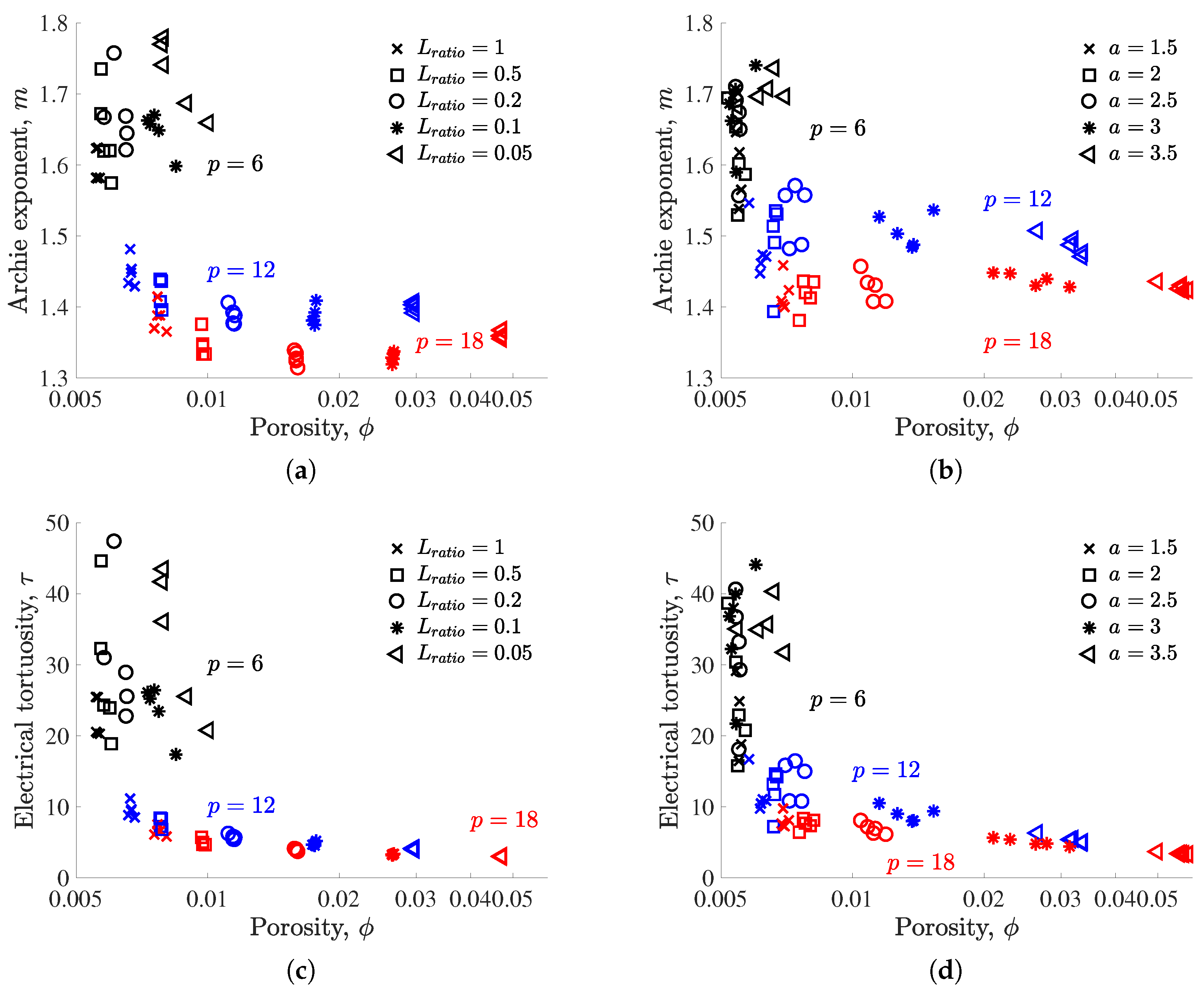
3. Results for Complex Fractured Porous Media

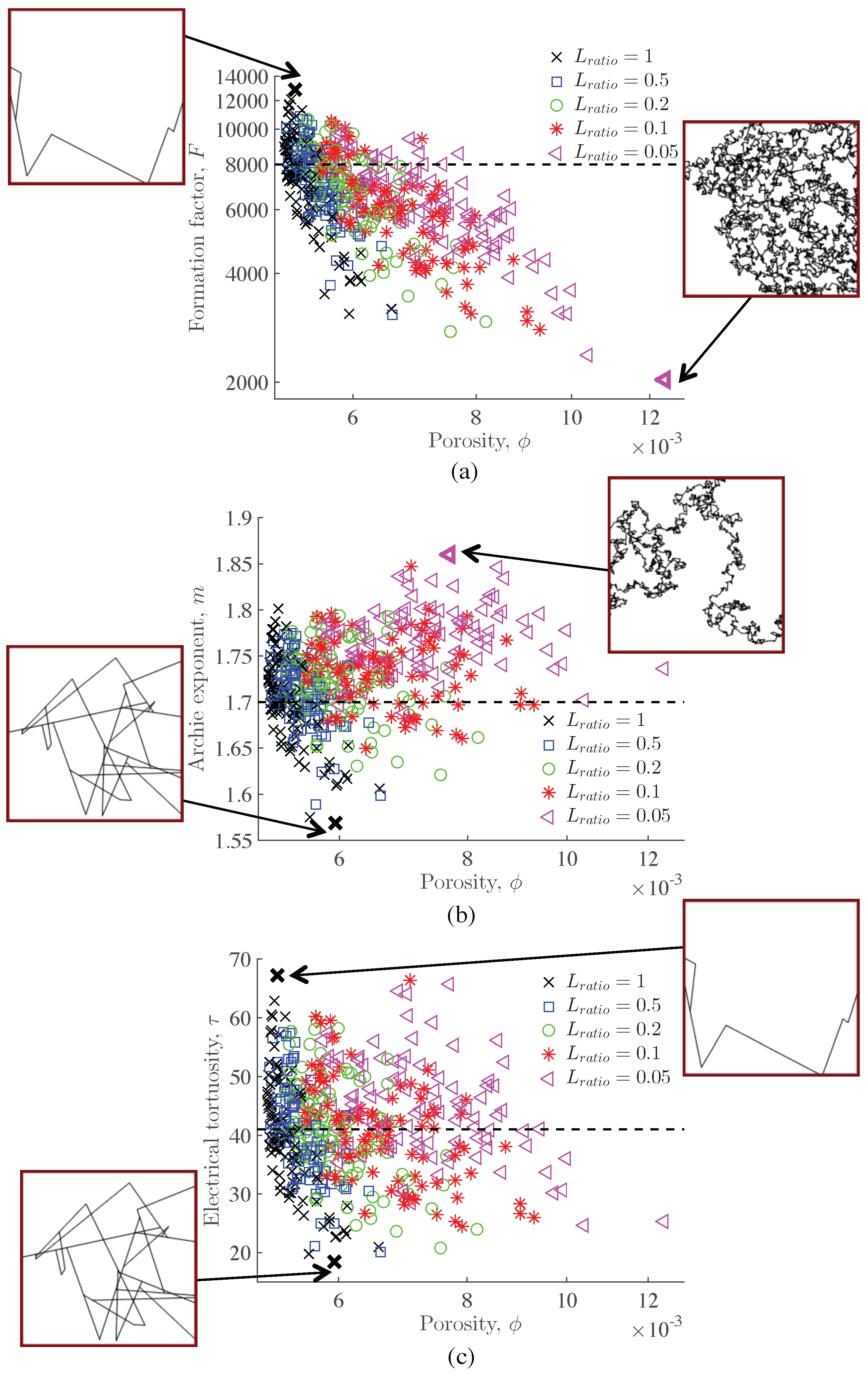
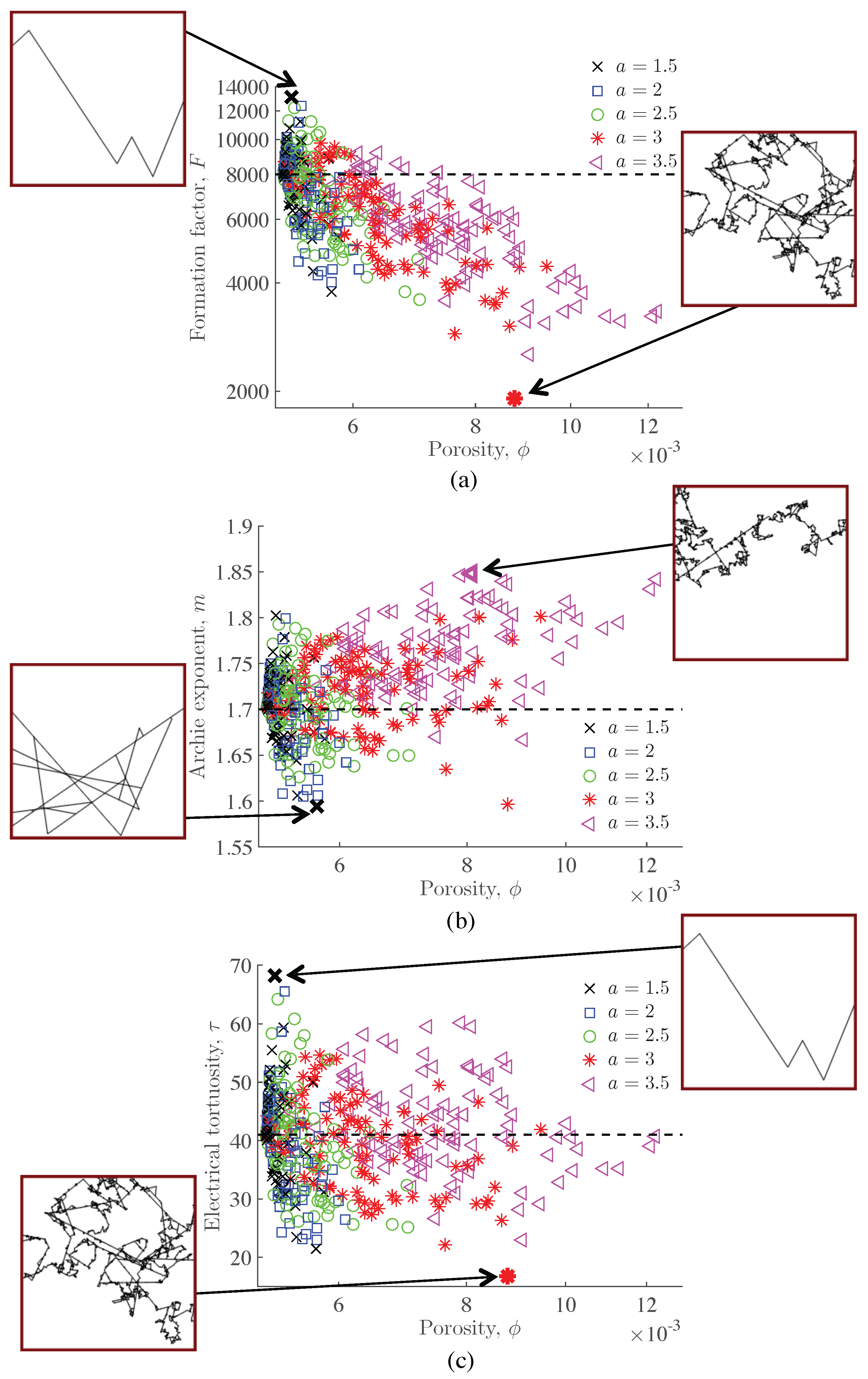
3.1. Results for a Large Range of Fracture Densities

For each family of fractures, that is, for each combination of the parameters {$L_{max}$,p} and {a,p}, five random fracture networks are generated and the electrical parameters F, m and $\tau$ are numerically evaluated as described in Section 2. The corresponding values of F are presented in Figure 2 and the values of m and $\tau$ are presented in Figure 3. In these figures, we see that decreasing the value of $L_{ratio}$, or increasing the value of a, for a given value of p, results in increasing the system porosity, because the fracture networks are characterized by smaller fractures (Figure 1). Clearly, the porosity $\varphi$ also increases when increasing p as this corresponds to adding more fractures to the systems (Figure 1).

In Figure 2, we observe that the electrical formation factor F decreases when $\varphi$ increases, and that the logarithms of these two parameters are not linearly related as typically assumed when using standard petrophysical relationships (Section 2.1). In order to understand this behavior, we compare these results to those obtained for simplified configurations. In particular, we consider a simple fracture–matrix system with $N_f$ horizontal fractures embedded in a matrix having domain size, fracture aperture and conductivity, and matrix porosity and conductivity as defined in Section 2.3. In such a domain, the fracture tortuosity is equal to its minimum value 1 and the electrical formation factor $F^{\ast }$ can be analytically expressed as $F^{\ast }=L/[N_f{b}_f+(L-N_f{b}_f){\varphi }_b^{m_b}]$. In Figure 2a,b, the scaled value $2.8F^{\ast }$ of simple fracture–matrix systems (black curve denoted as “Simple fracture–matrix systems”) is plotted as a function of the porosity $\varphi$ by varying $N_f$ from 0 to 500. This solution fits well the general tendency observed for our complex fracture–matrix systems, except for sparse fracture networks (i.e., $p=6$) characterized by the presence of small fractures (i.e., small values of $L_{ratio}$ in Figure 2a and large values of a in Figure 2b). We also observe that the fit between simple and complex systems is better when the fracture lengths are drawn from a uniform distribution (Figure 2a) than from a power-law distribution (Figure 2b). Finally, in these figures, we also represent the following simplified cases: (i) a domain with no fractures, that is, $N_f=0$, for which the domain porosity $\varphi$ is equal to the matrix porosity ${\varphi }_b$ and the reference electrical formation factor $F^{\ast }$ is expressed as $F^{\ast }={\varphi }^{-2}$ (“Matrix only” dashed line); and (ii) a domain with a matrix impervious to electrical current, that is, ${\sigma }_b={\varphi }_b^{-m_b}=0$, for which the domain porosity only depends on the fractures as $\varphi =N_f{b}_f/L$ implying that the reference electrical formation factor $F^{\ast }$ is expressed as $F^{\ast }={\varphi }^{-1}$ (“Fracture only” dashed line). Note that these simplified cases help to define bounds for fracture–matrix systems, as done with the Voigt and Reuss bounds in effective-medium theories [41].

Figure 2a,b show that the relationship between F and $\varphi$ for both complex (symbols) and simple (full black line) fracture–matrix systems is more complicated than Archie’s law $F={\varphi }^{-m}$ applied to either pure matrix ($m=2$, “Matrix only”) or pure fractures ($m=1$, “Fractures only”) configurations. The behavior of fracture–matrix systems is somewhere between these two laws where the contrast in topological and electrical properties between fractures and matrix impacts the effective electrical properties. More precisely, the analytical solution for simple fracture–matrix systems shows (i) a strong decrease in F when $\varphi$ ranges from 0.005 to 0.006, corresponding to configurations where adding fractures to a pure matrix system leads to small changes in $\varphi$ and large changes in F, because fractures are, at the same time, small and highly conductive structures in comparison with the matrix; and (ii) a slower decrease in F when $\varphi$ is larger than $0.006$, corresponding to configurations where the electrical properties are mostly determined by the fractures that are already present in the system, implying that adding new fractures leads to relatively small changes in these properties. This is also observed for complex fracture–matrix systems, except for sparse fracture networks with small fractures (i.e., $p=6$ with small values of $L_{ratio}$ and large values of a), implying that additional analysis is required to understand the complex fractured media considered in this study.

From here on, we focus on the behavior of these domains as a function of their fracture density, and we evaluate whether the Archie’s law formulations described in Section 2.1 may be used to describe the link between topological and electrical properties. For both uniformly and power-law-distributed fracture lengths,

Table 1. Parameters obtained by fitting the results in Figure 2 with the models $F={\varphi }^{-m^{\prime }}$ and $F={\tau }^{\prime }/\varphi$ using a non-linear least-squares method. Bold numbers show the best models for which the coefficient of determination $R^2$ is larger than 0.8. The corresponding models are plotted in Figure 2c,d.

		$\mathit{F}={\mathit{\varphi }}^{-{\mathit{m}}^{\prime }}$		$\mathit{F}={\mathit{\tau }}^{\prime }/\mathit{\varphi }$
		${\mathit{m}}^{\prime }$	${\mathit{R}}^{\mathbf{2}}$	${\mathit{\tau }}^{\prime }$	${\mathit{R}}^{\mathbf{2}}$
p (Figure 2c)	6	$1.65$	$0.06$	$27.79$	$0.18$
	12	$\mathbf{1.43}$	$\mathbf{0.95}$	$7.98$	$0.85$
	18	$\mathbf{1.37}$	$\mathbf{0.96}$	$5.55$	$0.89$
p (Figure 2d)	6	$1.66$	$-0.06$	$30.47$	0
	12	$\mathbf{1.5}$	$\mathbf{0.83}$	$12.4$	$0.81$
	18	$\mathbf{1.42}$	$\mathbf{0.97}$	$7.56$	$0.94$

shows that (i) when $p=6$, the relationship between F and $\varphi$ cannot be described by the Archie’s law formulations $F={\varphi }^{-m^{\prime }}$ or $F={\tau }^{\prime }/\varphi$, as the coefficient of determination R is smaller than $0.2$; and (ii) when $p=12$ and 18, both formulations lead to a satisfying fit of the data, as R is larger than $0.8$. In the latter cases, the standard formulation $F={\varphi }^{-m^{\prime }}$ provides the best models with $m^{\prime }$ ranging between $1.3$ and $1.5$. These results show that, for configurations with a high fracture density, the cementation factor $m^{\prime }$ offers a better description than the tortuosity ${\tau }^{\prime }$, where $m^{\prime }$ decreases when increasing the fracture density (from $p=12$ to $p=18$) and when decreasing the fracture network complexity (from power-law- to uniformly distributed fracture lengths). These results also show that complex fracture–matrix systems characterized by sparse fracture networks (i.e., $p=6$) cannot be described by standard petrophysical relationships, as the density of fractures is not high enough to reach a representative elementary volume.

Finally, we consider the electrical parameters m and $\tau$ defined in (1) for complex fracture–matrix systems (Figure 3) in order to evaluate whether these parameters can bring information on the topological properties of the studied systems. For instance, we see that the values of the Archie’s exponent m, which range between $1.3$ and $1.8$, tend to increase when (i) p decreases; and (ii) for $p=6$, when $L_{ratio}$ decreases (Figure 3a) and when a increases (Figure 3b). This is consistent with existing studies showing that m characterizes how the electric current samples the interconnected porosity as follows: (i) Small values of m are expected for fractured domains with interconnected open fractures where the electrical charges are transported through most of the porosity; and (ii) large values of m are expected for domains with large pores connected by narrow throats where the electrical charges are poorly transported in some parts of the porosity (e.g., [22,29]). In our case, large values of p correspond to a high density of fractures which gives access to most of the porosity. Conversely, small values of p associated with the presence of small fractures result in sparse fracture networks for which some parts of the domain are difficult to access.

Different behavior between the $p=6$ and $p\ge 12$ cases is also observed for the electrical tortuosity $\tau$ (Figure 3c,d). For the considered fracture–matrix systems, $\tau$, which ranges between 3 and 50, increases when p decreases because the complexity of the path followed by the electric current is greater when a smaller density of fractures connects the left and right sides of the domain (Figure 1). We also observe that, for both m and $\tau$, the high variability of the results obtained for $p=6$ suggests that a large quantity of data are required to investigate the behavior of these systems, which are comprised of fracture networks that are at (or very close to) the percolation threshold [51].

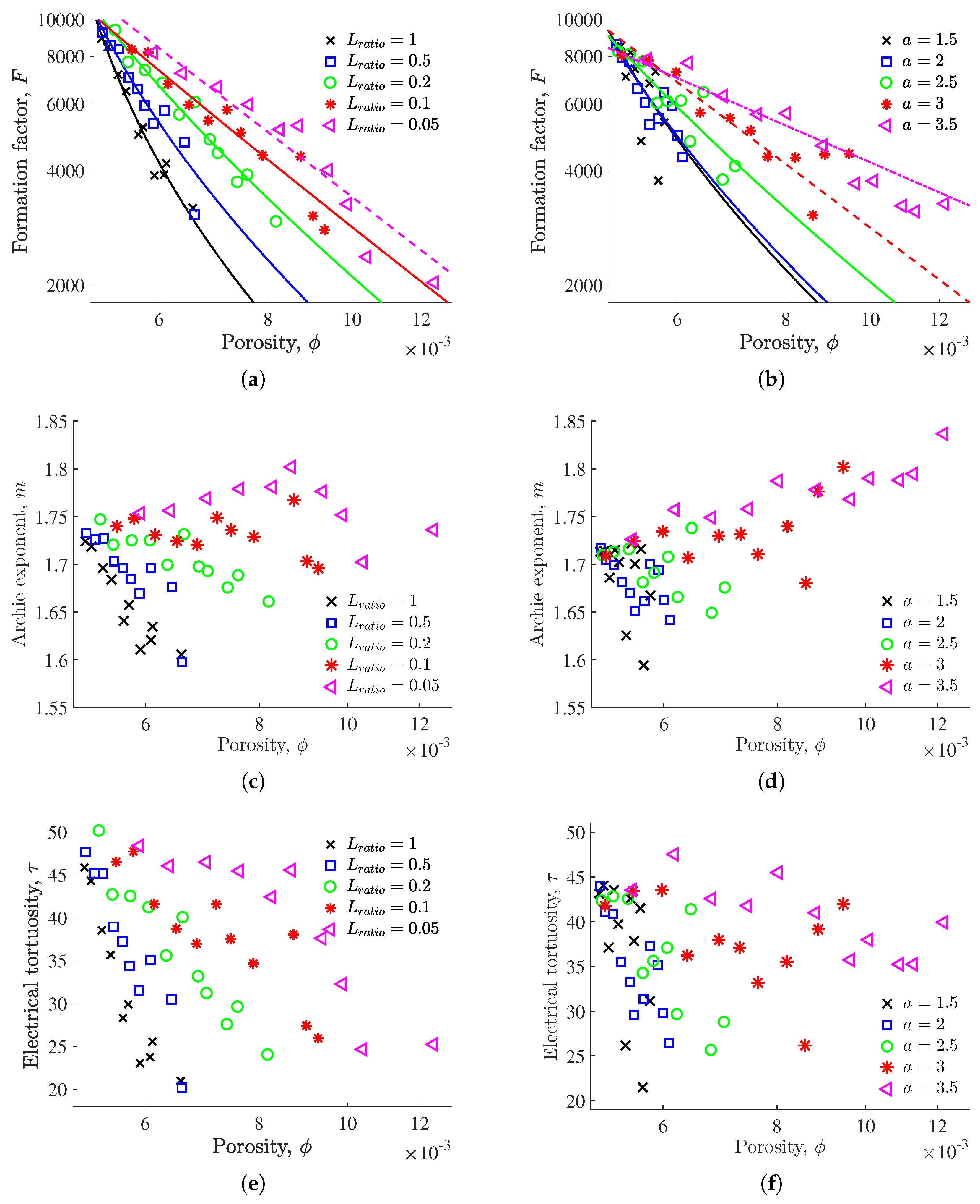
3.2. Results at the Fracture Percolation Threshold

In order to gain a better understanding of the results obtained in Section 3.1 for low-porosity fracture–matrix systems (i.e., $p=6$), we consider 100 random fracture networks at the percolation threshold for each family of fractures (i.e., for each value of $L_{ratio}$ and a). As before, we evaluate parameters F, m and $\tau$ using (1). The obtained results are shown in Figure 4 and Figure 5 considering a uniform and power-law distribution for the fracture lengths, respectively. In these figures, we also show the fracture–matrix systems leading to the minimum and maximum values of the evaluated electrical parameters, as well as the reference electrical parameters $F_1^{\ast }=8000$, $m_1^{\ast }=1.7$ and ${\tau }_1^{\ast }=41$ (dashed black lines) that are obtained for a single horizontal fracture embedded into a conductive matrix considering the properties described in Section 2.3, the analytical solution provided in Section 3.1 for $F^{\ast }$, and Expressions (1).

The results presented in Figure 4 and Figure 5 show a large range in the obtained values of F, m and $\tau$, which is related to the properties of the considered fracture networks and the contrast in properties between the fractures and matrix. For instance, Figure 4a and Figure 5a show that the maximum and minimum values of F are larger and smaller than $F_1^{\ast }$, respectively, implying that these systems are less and more conductive than the considered reference system, respectively (Expressions (1)). The maximum values of F are associated with simple fracture networks that are characterized by a few long fractures, whereas the minimum values are associated with complex fracture networks that are characterized by the presence of small fractures. In both cases, the tortuosity of these fracture networks implies that they are less conductive than a single horizontal fracture. However, when these fracture networks are embedded into a conductive matrix, the quantity of fractures and their spatial distribution throughout the system impact the overall conductivity of the fracture–matrix systems. When a few long fractures are embedded into the matrix, these fractures do not affect the overall conductivity, implying that the effective electrical conductivity of these systems is smaller than that of a single fracture embedded into a matrix. Conversely, when many fractures are embedded throughout the matrix, they contribute to the overall conductivity, implying that the effective electrical conductivity of these systems is larger than the reference fracture–matrix system. This shows that the considered large ranges of fracture-network properties result in large ranges in the formation factor F with a strong impact of the fracture length and distribution, as well as of the fracture–matrix exchanges.

As shown in Figure 4 and Figure 5, these properties and processes also impact the obtained values of m and $\tau$. In particular, from the definition of these parameters in (1), small values of m and $\tau$ are associated with small values of F and $\varphi$, which correspond to highly conductive domains characterized by a small porosity. This implies that the minimum values of m and $\tau$ are related to fracture–matrix systems that optimize the ratio of conductivity to porosity, which is observed here for relatively long fractures that are spatially distributed throughout the systems (Figure 4b,c and Figure 5b). Note that, in Figure 5c, the fracture network associated with the smallest value of $\tau$ is composed of fractures of various lengths. In this case, the relatively large value of porosity related to these structures is counterbalanced by the high conductivity of the overall system, as this configuration is associated with the smallest value of F (Figure 5a). Conversely, the maximum values of m are associated with systems that are characterized by the presence of small fractures, which either form (Figure 4b), or are localized along (Figure 5b), the conductive fracture path. This corresponds to configurations for which the porosity value is maximized while the conductivity is minimized. Finally, fractured porous domains associated with the maximum values of $\tau$ are the same as the domains associated with the maximum values of F (Figure 4c and Figure 5c). Although these configurations present small porosities, the product $F\times \varphi$ is optimized by the large values of F.

Finally, in order to improve the readability and interpretation of the results presented in Figure 4 and Figure 5, we averaged the computed electrical parameters for each family of fractures. This was done by discretizing the corresponding porosity ranges into 10 intervals and averaging the values of the electrical parameters included in each interval. Figure 6 shows the resulting values and

Table 2. Parameters obtained by fitting the results in Figure 6a,b with the models $F={\varphi }^{-m^{\prime }}$, $F={\tau }^{\prime }/\varphi$ and $F={(\varphi -{\varphi }_c)}^{-t}$ using a non-linear least-squares method. Bold numbers show the best models for which the coefficient of determination $R^2$ is larger than 0.8. The best model of each configuration is plotted in Figure 6a,b.

		$\mathit{F}={\mathit{\varphi }}^{-{\mathit{m}}^{\prime }}$		$\mathit{F}={\mathit{\tau }}^{\prime }/\mathit{\varphi }$		$\mathit{F}={(\mathit{\varphi }-{\mathit{\varphi }}_{\mathit{c}})}^{-\mathit{t}}$
		${\mathit{m}}^{\prime }$	${\mathit{R}}^{\mathbf{2}}$	${\mathit{\tau }}^{\prime }$	${\mathit{R}}^{\mathbf{2}}$	${\mathit{\varphi }}_{\mathit{c}}$	$\mathit{t}$	${\mathit{R}}^{\mathbf{2}}$
$L_{ratio}$ (Figure 6a)	1	$1.68$	$0.56$	33	$0.36$	$\mathbf{0.004}$	$\mathbf{1.33}$	$\mathbf{0.98}$
	$0.5$	$1.7$	$0.69$	38	$0.46$	$\mathbf{0.003}$	$\mathbf{1.44}$	$\mathbf{0.94}$
	$0.2$	$1.72$	$0.88$	38	$0.62$	$\mathbf{0.002}$	$\mathbf{1.57}$	$\mathbf{0.96}$
	$0.1$	1.74	$0.94$	40	$0.75$	$\mathbf{0.0006}$	$\mathbf{1.7}$	$\mathbf{0.95}$
	$0.05$	1.77	0.94	42	$0.79$	$\mathbf{2}\times {\mathbf{10}}^{-\mathbf{11}}$	1.77	0.94
a (Figure 6b)	$1.5$	$1.7$	$0.33$	37	$0.22$	$0.003$	$1.44$	$0.47$
	2	$1.69$	$0.64$	35	$0.43$	$\mathbf{0.003}$	$\mathbf{1.46}$	$\mathbf{0.83}$
	$2.5$	$1.7$	$0.78$	37	$0.57$	$\mathbf{0.002}$	$\mathbf{1.59}$	$\mathbf{0.83}$
	3	$\mathbf{1.73}$	$\mathbf{0.84}$	39	$0.82$	${\mathbf{10}}^{-\mathbf{11}}$	$\mathbf{1.73}$	$\mathbf{0.84}$
	$3.5$	$1.76$	$0.85$	42	$\mathbf{0.92}$	$5\times {10}^{-12}$	$1.76$	$0.85$

gives the parameters associated with three models that are used to reproduce the relationships between F and $\varphi$ for each value of $L_{ratio}$ and a. As before, we use the two Archie’s law formulations $F={\varphi }^{-m^{\prime }}$ and $F={\tau }^{\prime }/\varphi$. In addition, we consider the percolation-theory model $F={(\varphi -{\varphi }_c)}^{-t}$ (e.g., [31,52,53]), in order to evaluate whether the notion of a critical porosity ${\varphi }_c$ helps to interpret data corresponding to low-porosity fractured porous media with sparse fracture networks. Note that in this case, the estimated value of ${\varphi }_c$ is restricted to lie between 0 and the minimum porosity of the considered fracture family.

Figure 6 shows the trends of the electrical parameters F, m and $\tau$, which are related to the fracture-network parameters $L_{ratio}$ and a. For instance, for each value of these latter parameters, we observe that F tends to decrease when $\varphi$ increases, which corresponds to an increase in the system conductivity when adding fractures to the system (Figure 6a,b). We also observe that m tends to decrease when $\varphi$ increases for large and small values of $L_{ratio}$ and a, respectively, and shows some increases for small and large values of $L_{ratio}$ and a, respectively. This is consistent with the definition of m found in the literature and explained in Section 2.1, which considers that m describes how the electric current samples the interconnected porosity. In our case, adding fractures to systems that are characterized by long fractures leads to a better sampling of the interconnected porosity, and thus to a decrease in m. Conversely, adding fractures to systems that are characterized by the presence of small fractures can result in creating localized areas that are difficult to access, implying potential increases in m. Finally, $\tau$ tends to decrease or stabilize when $\varphi$ increases, implying that adding fractures to the considered fracture–matrix systems reduces the overall electrical tortuosity. From the definition of $\tau$ provided in (1), the observed behavior of $\tau$ is related to that of F, and the impact of $\varphi$ is limited as adding fractures into the considered systems results in small changes in porosity in comparison with the corresponding changes in F.

The values presented in Table 2 show that the percolation-theory model is generally more adequate than Archie’s law to describe the relationship between F and $\varphi$ for fracture–matrix systems that are characterized by a fracture network at the percolation threshold. This observation is expected because the applicability of relationships such as Archie’s law relies on the existence of a representative elementary volume, which is unlikely for low-porosity fracture–matrix systems with sparse fracture networks. However, our results also demonstrate that (i) the standard formulation of Archie’s law leads to satisfying models (i.e., $R^2>0.8$) for $L_{ratio}=0.2$, $0.1$ and $0.05$, and $a=3$ and $3.5$; (ii) the formulation $F={\tau }^{\prime }/\varphi$ provides the best model for $a=3.5$; and (iii) the percolation-theory model and the formulation $F={\varphi }^{-m^{\prime }}$ are equally adequate (i.e., same value of $R^2$) when $L_{ratio}=0.05$, and $a=3$ and $3.5$. Consequently, although fracture networks at the percolation threshold are usually associated with sparse distributions of fractures implying that Archie’s law will not hold for the resulting fracture–matrix systems, this statement is questionable when the considered systems are characterized by the presence of small fractures that interact with the surrounding matrix.

4. Discussion

We have presented in this paper a numerical analysis of the electrical parameters F, m and $\tau$, which are commonly used to characterize the relationship between topological and electrical properties, for low-porosity complex and realistic fracture–matrix systems. In this regard, we examined a large range of fracture networks with varying fracture densities and length distributions. We compared these domains to simple fracture–matrix systems consisting of horizontal fractures embedded into a conductive matrix, and evaluated whether standard petrophysical relationships such as Archie’s law are applicable. We also investigated whether the electrical parameters provide information on the fracture network properties, such as fracture density, length and spatial distribution.

Considering a large range of porosities through the consideration of various fracture densities, our results show that the electrical formation factor F of fractured rocks exhibits a more complicated behavior than that of pure-fracture and pure-matrix systems. For both simple and complex fracture–matrix systems, this behavior is related to the contrast in topological and electrical properties between matrix and fractures, where the properties of both structures impact the electrical parameters.

That being said, considering only high fracture densities leads to simplified behaviors that can be described with Archie’s law, and for which Archie’s exponent m depends on the fracture density and fracture length heterogeneity. More precisely, decreasing values of m obtained over various fractured rock samples can be related to an increase in fracture density, if the fracture length heterogeneities are assumed similar over the considered samples, or to a decrease in the fracture network complexity, otherwise.

Conversely, considering fracture networks that are at (or close to) the percolation threshold leads to highly variable results, for which the applicability of standard petrophysical relationships is questionable. In this case, conducting our study over a large number of simulations shows that, although we consider a very low-porosity matrix, the fracture–matrix exchanges have a critical impact on the obtained electrical parameters. For instance, the impact of the fracture network tortuosity is diminished when the network is characterized by the presence of small fractures that are spatially distributed throughout the matrix, because these fractures contribute to the overall properties through fracture–matrix exchanges. Furthermore, considering the averaged electrical parameters for each family of fractures (i.e., for a given definition of the fracture-length distribution), the relationship between F and $\varphi$ is generally well described by percolation-theory models, but can also be described by Archie’s law when the fracture networks are characterized by the presence of small fractures. We also observe that the behavior of the electrical parameters m and $\tau$ along porosity changes can help to identify the fracture-network properties. A standard behavior of these parameters is observed, that is, m and $\tau$ decrease when $\varphi$ increases, when the fracture networks are characterized by long fractures. Conversely, more complex behaviors are observed when these networks are characterized by the presence of small fractures with, for instance, an increase in m, and increases and decreases in $\tau$, when the fracture lengths are described from a power-law distribution. This is consistent with existing studies on porous systems, as larger values of m and $\tau$ are expected when the porosity is difficult to sample and the electric current follows complicated paths, which is the case for fracture-network systems characterized by the presence of small fractures.

Finally, our results are also consistent with laboratory experiments that are conducted on low-porosity fractured samples, and bring new insights to understand them. For the non-granoblastic dikes and gabbros studied in [35], the electrical parameters m and $\tau$ increase when the porosity increases, and these parameters are smaller for gabbros than for non-granoblastic dikes. This is related to the topological properties of these samples because gabbros contain numerous fissures and cracks resulting in open localized connections, and non-granoblastic dikes are generally altered with relatively high and interconnected porosity. This is equivalent to our synthetic systems characterized either by long fractures or by the presence of small fractures, with an increase in m and $\tau$ when the porosity increase is related to the transition from the former configuration to the latter. Gabbros have also been studied in [33] collecting rock samples along a borehole. This results in observing different values of the electrical parameters between the upper and lower parts of the considered well. In the upper part, m increases with $\varphi$ and $\tau$ remains constant, whereas in the lower part, low values of $\varphi$, m and $\tau$ are observed. The authors suggested that these observations are related to a porous network that is controlled by primary microstructures in the upper part, and by the presence of dominant well-aligned cracks in the lower part. This is confirmed by our results considering that the former configurations correspond to the presence of small fractures, and the latter to systems whose properties are defined by long and connecting fractures. These different structures are also assumed in Le Pennec et al. [22] to explain the electrical parameters and their behavior obtained for angular blocks and scoria fragments sampled in block-and-ash flow deposits of the Merapi volcano. Finally, the increasing values of the electrical tortuosity observed in Pezard et al. [34] for small increasing values of the porosity are more likely related to the large variability of the electrical parameters in these structures and to the study of samples characterized by various ranges of fracture lengths.

5. Conclusions

In order to improve our understanding of previous laboratory measurements made on fractured rocks, the current study relates the porosity and effective electrical conductivity of a wide variety of synthetic fractured rock samples. This work focuses on the impact of the fracture-network organization and density with heterogeneous fracture lengths, assuming that the fractures are highly conductive structures having constant aperture and embedded in a constant-porosity matrix. Extensions to this work should focus on systems that are more representative of the natural environment, for example by considering heterogeneous fracture apertures. It is expected that these more realistic synthetic systems will exhibit more complex behaviors of the electrical parameters described in our work. More realistic representations of the natural environment could also be achieved by considering that fractures may also act as barriers which deviate fluids and potentially reduce the effective electrical conductivity of the considered systems [54].

Finally, the laboratory experiments considered in this work imply that the effective electrical conductivity is evaluated and analyzed in one direction. However, our methodology could also be applied to study the anisotropy of heterogeneous fractured rocks by computing their effective electrical conductivity in various directions. This can be used to test whether a tensorial representation of this property is appropriate and to relate this property to the anisotropic orientation of the considered fracture networks. New insights obtained from the present study and future work should also be compared to conclusions provided by existing studies on composite domains which are based on effective-medium theories.

References

1. Garg, S.K.; Pritchett, J.W.; Wannamaker, P.E.; Combs, J. Characterization of geothermal reservoirs with electrical surveys: Beowawe geothermal field. Geothermics 2007, 36, 487–517. [Google Scholar] [CrossRef]
2. Kazakis, N.; Vargemezis, G.; Voudouris, K.S. Estimation of hydraulic parameters in a complex porous aquifer system using geoelectrical methods. Sci. Total Environ. 2016, 550, 742–750. [Google Scholar] [CrossRef] [PubMed]
3. Priegnitz, M.; Thaler, J.; Spangenberg, E.; Schicks, J.M.; Schroetter, J.; Abendroth, S. Characterizing electrical properties and permeability changes of hydrate bearing sediments using ERT data. Geophys. J. Int. 2015, 202, 1599–1612. [Google Scholar] [CrossRef]
4. Carneiro, J.F. Numerical simulations on the influence of matrix diffusion to carbon sequestration in double porosity fissured aquifers. Int. J. Greenh. Gas Control 2009, 3, 431–443. [Google Scholar] [CrossRef]
5. Kolditz, O.; Clauser, C. Numerical simulation of flow and heat transfer in fractured crystalline rocks: Application to the Hot Dry Rock site in Rosemanowes (U.K.). Geothermics 1998, 27, 1–23. [Google Scholar] [CrossRef]
6. Lee, M.W.; Collett, T.S. Gas hydrate saturations estimated from fractured reservoir at Site NGHP-01-10, Krishna-Godavari Basin, India. J. Geophys. Res. Solid Earth 2009, 114. [Google Scholar] [CrossRef]
7. Berkowitz, B. Characterizing flow and transport in fractured geological media: A review. Adv. Water Resour. 2002, 25, 861–884. [Google Scholar] [CrossRef]
8. Bonnet, E.; Bour, O.; Odling, N.E.; Davy, P.; Main, I.; Cowie, P.; Berkowitz, B. Scaling of fracture systems in geological media. Rev. Geophys. 2001, 39, 347–383. [Google Scholar] [CrossRef] [Green Version]
9. Neuman, S. Trends, prospects and challenges in quantifying flow and transport through fractured rocks. Hydrogeol. J. 2005, 13, 124–147. [Google Scholar] [CrossRef]
10. Dorn, C.; Linde, N.; Le Borgne, T.; Bour, O.; de Dreuzy, J.R. Conditioning of stochastic 3-D fracture networks to hydrological and geophysical data. Adv. Water Resour. 2013, 62, 79–89. [Google Scholar] [CrossRef]
11. Le Borgne, T.; Bour, O.; Riley, M.S.; Gouze, P.; Pezard, P.A.; Belghoul, A.; Lods, G.; Le Provost, R.; Greswell, R.B.; Ellis, P.A.; et al. Comparison of alternative methodologies for identifying and characterizing preferential flow paths in heterogeneous aquifers. J. Hydrol. 2007, 345, 134–148. [Google Scholar] [CrossRef]
12. Lofi, J.; Pezard, P.; Loggia, D.; Garel, E.; Gautier, S.; Merry, C.; Bondabou, K. Geological discontinuities, main flow path and chemical alteration in a marly hill prone to slope instability: Assessment from petrophysical measurements and borehole image analysis. Hydrol. Process. 2012, 26. [Google Scholar] [CrossRef]
13. Daily, W.D.; Ramirez, A.L. In situ porosity distribution using geophysical tomography. Geophys. Res. Lett. 1984, 11, 614–616. [Google Scholar] [CrossRef]
14. Kazatchenko, E.; Mousatov, A. Primary and Secondary Porosity Estimation of Carbonate Formations Using Total Porosity and the Formation Factor. Soc. Pet. Eng. 2002. [Google Scholar] [CrossRef]
15. Whitman, D.; Yeboah-Forson, A. Electrical resistivity and porosity structure of the upper Biscayne Aquifer in Miami-Dade County, Florida. J. Hydrol. 2015, 531, 781–791. [Google Scholar] [CrossRef]
16. Archie, G. The electrical resistivity log as an aid in determining some reservoir characteristics. Trans. Am. Inst. Min. Metall. Eng. 1942, 146, 54–61. [Google Scholar] [CrossRef]
17. Katsube, T.J.; Hume, J.P. Permeability determination in crystalline rocks by standard geophysical logs. Geophysics 1987, 52, 342–352. [Google Scholar] [CrossRef]
18. Pezard, P.A.; Luthi, S.M. Borehole electrical images in the basement of the Cajon Pass Scientific Drillhole, California; Fracture identification and tectonic implications. Geophys. Res. Lett. 1988, 15, 1017–1020. [Google Scholar] [CrossRef]
19. Boadu, F.; Gyamfi, J.; Owusu, E. Determining subsurface fracture characteristics from azimuthal resistivity surveys: A case study at Nsawam, Ghana. Geophysics 2005, 70, B35–B42. [Google Scholar] [CrossRef]
20. Caballero Sanz, V.; Roubinet, D.; Demirel, S.; Irving, J. 2.5-D discrete-dual-porosity model for simulating geoelectrical experiments in fractured rock. Geophys. J. Int. 2017, 209, 1099–1110. [Google Scholar] [CrossRef]
21. Lesparre, N.; Boyle, A.; Grychtol, B.; Cabrera, J.; Marteau, J.; Adler, A. Electrical resistivity imaging in transmission between surface and underground tunnel for fault characterization. J. Appl. Geophys. 2016, 128, 163–178. [Google Scholar] [CrossRef]
22. Le Pennec, J.L.; Hermitte, D.; Dana, I.; Pezard, P.; Coulon, C.; Cochemé, J.J.; Mulyadi, E.; Ollagnier, F.; Revest, C. Electrical conductivity and pore-space topology of Merapi Lavas: Implications for the degassing of porphyritic andesite magmas. Geophys. Res. Lett. 2001, 28, 4283–4286. [Google Scholar] [CrossRef]
23. Liu, Y.; Xue, Z.; Park, H.; Kiyama, T.; Zhang, Y.; Nishizawa, O.; Chae, K.S. Measurement of electrical impedance of a Berea sandstone core during the displacement of saturated brine by oil and CO2 injections. J. Appl. Geophys. 2015, 123, 50–62. [Google Scholar] [CrossRef]
24. Sen, P.N.; Scala, C.; Cohen, M.H. A self-similar model for sedimentary rocks with application to the dielectric constant of fused glass beads. Geophysics 1981, 46, 781–795. [Google Scholar] [CrossRef]
25. Wright, H.M.; Cashman, K.V. Compaction and gas loss in welded pyroclastic deposits as revealed by porosity, permeability, and electrical conductivity measurements of the Shevlin Park Tuff. Geol. Soc. Am. Bull. 2014, 126, 234–247. [Google Scholar] [CrossRef]
26. Al-Ghamdi, A.; Chen, B.; Behmanesh, H.; Qanbari, F.; Aguilera, R. An Improved Triple-Porosity Model for Evaluation of Naturally Fractured Reservoirs. SPE Reserv. Eval. Eng. 2011, 14, 397–404. [Google Scholar] [CrossRef]
27. Bauer, D.; Youssef, S.; Han, M.; Bekri, S.; Rosenberg, E.; Fleury, M.; Vizika, O. From computed microtomography images to resistivity index calculations of heterogeneous carbonates using a dual-porosity pore-network approach: Influence of percolation on the electrical transport properties. Phys. Rev. E 2011, 84, 011133. [Google Scholar] [CrossRef] [PubMed]
28. Glover, P.W.J. A generalized Archie’s law for n phases. Geophysics 2010, 75, E247–E265. [Google Scholar] [CrossRef]
29. Revil, A.; Cathles, L.M. Permeability of shaly sands. Water Resour. Res. 1999, 35, 651–662. [Google Scholar] [CrossRef]
30. Torskaya, T.; Shabro, V.; Torres-Verdín, C.; Salazar-Tio, R.; Revil, A. Grain Shape Effects on Permeability, Formation Factor, and Capillary Pressure from Pore-Scale Modeling. Transp. Porous Media 2013, 102, 71–90. [Google Scholar] [CrossRef]
31. Ghanbarian, B.; Hunt, A.G.; Ewing, R.P.; Skinner, T.E. Universal scaling of the formation factor in porous media derived by combining percolation and effective medium theories. Geophys. Res. Lett. 2014, 41, 3884–3890. [Google Scholar] [CrossRef]
32. Winsauer, W.O. Resistivity of brine-saturated sands in relation to pore geometry. AAPG Bull. 1952, 36, 253–277. [Google Scholar]
33. Ildefonse, B.; Pezard, P. Electrical properties of slow-spreading ridge gabbros from ODP Site 735, Southwest Indian Ridge. Tectonophysics 2001, 330, 69–92. [Google Scholar] [CrossRef]
34. Pezard, P.; Ito, H.; Hermitte, D.; Revil, A. Electrical properties and alteration of granodiorites from the GSJ Hirabayashi Hole, Japan. In Proceedings of the International Workshop of the Nojima Fault Core and Borehole Data Analysis, Tsukuba, Japan, 22–23 November 1999; Geological Survey of Japan; Number EQ/00/1 in USGS Open-File Report 000-129. Ito, H., Fujimoto, K., Tanaka, H., Lockner, D., Eds.; pp. 255–262. [Google Scholar]
35. Violay, M.; Pezard, P.A.; Ildefonse, B.; Belghoul, A.; Laverne, C. Petrophysical properties of the root zone of sheeted dikes in the ocean crust: A case study from Hole ODP/IODP 1256D, Eastern Equatorial Pacific. Tectonophysics 2010, 493, 139–152. [Google Scholar] [CrossRef]
36. Berg, C.R. Dual-Porosity Equations From Effective Medium Theory. In Proceedings of the SPE Annual Technical Conference and Exhibition, San Antonio, TX, USA, 24–27 September 2006; Society of Petroleum Engineers: Richardson, TX, USA, 2006. [Google Scholar]
37. Long, J.C.S.; Remer, J.S.; Wilson, C.R.; Witherspoon, P.A. Porous media equivalents for networks of discontinuous fractures. Water Resour. Res. 1982, 18, 645–658. [Google Scholar] [CrossRef]
38. De Dreuzy, J.R.; Davy, P.; Bour, O. Hydraulic properties of two-dimensional random fracture networks following a power law length distribution: 1. Effective connectivity. Water Resour. Res. 2001, 37, 2065–2078. [Google Scholar] [CrossRef]
39. Roubinet, D.; de Dreuzy, J.R.; Davy, P. Connectivity-consistent mapping method for 2-D discrete fracture networks. Water Resour. Res. 2010, 46, W07532. [Google Scholar] [CrossRef]
40. De Dreuzy, J.R.; Davy, P.; Bour, O. Hydraulic properties of two-dimensional random fracture networks following a power law length distribution: 2. Permeability of networks based on lognormal distribution of apertures. Water Resour. Res. 2001, 37, 2079–2095. [Google Scholar] [CrossRef]
41. Schön, J. Physical Properties of Rocks. In Physical Properties of Rocks-A Workbook; Schön, J., Ed.; Elsevier: Amsterdam, The Netherlands, 2011; Volume 8. [Google Scholar]
42. Walsh, J.B.; Brace, W.F. The effect of pressure on porosity and the transport properties of rock. J. Geophys. Res. Solid Earth 1984, 89, 9425–9431. [Google Scholar] [CrossRef]
43. Pape, H.; Riepe, L.; Schopper, J.R. Petrophysical Detection Of Microfissures In Granites. In Proceedings of the Society of Petrophysicists and Well-Log Analysts (SPWLA) 26th Annual Logging Symposium, Dallas, TX, USA, 17–20 June 1985. [Google Scholar]
44. Selley, R.C.; Sonnenberg, S.A. (Eds.) Chapter 3-Methods of Exploration. In Elements of Petroleum Geology, 3rd ed.; Academic Press: Boston, MA, USA, 2015; pp. 41–152. [Google Scholar]
45. Selley, R.C.; Sonnenberg, S.A. (Eds.) Chapter 6-The Reservoir. In Elements of Petroleum Geology, 3rd ed.; Academic Press: Boston, MA, USA, 2015; pp. 255–320. [Google Scholar]
46. Wright, H.M.; Cashman, K.V.; Gottesfeld, E.H.; Roberts, J.J. Pore structure of volcanic clasts: Measurements of permeability and electrical conductivity. Earth Planet. Sci. Lett. 2009, 280, 93–104. [Google Scholar] [CrossRef]
47. Pezard, P.A. Electrical properties of mid-ocean ridge basalt and implications for the structure of the upper oceanic crust in Hole 504B. J. Geophys. Res. Solid Earth 1990, 95, 9237–9264. [Google Scholar] [CrossRef]
48. Sunberg, K. Effect on impregnating waters on electrical conductivity of soils and rocks. Trans. Am. Inst. Min. Metal. Eng. 1932, 79, 367–391. [Google Scholar]
49. Brace, W.F.; Orange, A.S.; Madden, T.R. The effect of pressure on the electrical resistivity of water-saturated crystalline rocks. J. Geophys. Res. 1965, 70, 5669–5678. [Google Scholar] [CrossRef]
50. Roubinet, D.; Irving, J. Discrete-dual-porosity model for electric current flow in fractured rock. J. Geophys. Res. Solid Earth 2014, 119, 767–786. [Google Scholar] [CrossRef]
51. Bour, O.; Davy, P. Connectivity of random fault networks following a power law fault length distribution. Water Resour. Res. 1997, 33, 1567–1583. [Google Scholar] [CrossRef]
52. Markov, M.; Mousatov, A.; Kazatchenko, E.; Markova, I. Determination of electrical conductivity of double-porosity formations by using generalized differential effective medium approximation. J. Appl. Geophys. 2014, 108, 104–109. [Google Scholar] [CrossRef]
53. Daigle, H.; Ghanbarian, B.; Henry, P.; Conin, M. Universal scaling of the formation factor in clays: Example from the Nankai Trough. J. Geophys. Res. Solid Earth 2015, 120, 7361–7375. [Google Scholar] [CrossRef]
54. Faulkner, D.; Jackson, C.; Lunn, R.; Schlische, R.; Shipton, Z.; Wibberley, C.; Withjack, M. A review of recent developments concerning the structure, mechanics and fluid flow properties of fault zones. J. Struct. Geol. 2010, 32, 1557–1575. [Google Scholar] [CrossRef]
Figure 1. Interconnected fracture networks for the domains whose fracture lengths are defined by (af) a uniform distribution with L r a t i o = L m a x / L ; and (gl) a power-law distribution.
Minerals 08 00014 g001
Figure 2. Electrical formation factor F plotted as a function of porosity ϕ with the fracture lengths being defined from uniform (left column) and power-law (right column) distributions. The fracture networks are generated with the percolation parameter p = 6 , 12 and 18 (black, blue and red symbols, respectively), and we consider 5 simulations for each combination of the parameters { L m a x ,p} and {a,p}. The relationship between F and ϕ is compared to (a,b) values obtained for simple configurations that are described in the text, and (c,d) models based on Archie’s law that are described in Table 1.
Minerals 08 00014 g002aMinerals 08 00014 g002b
Figure 3. (a,b) Archie’s exponent m and (c,d) electrical tortuosity τ plotted as a function of porosity ϕ with the fracture lengths being defined from uniform (left column) and power-law (right column) distributions. These electrical parameters are computed from the results presented in Figure 2.
Minerals 08 00014 g003
Figure 4. (a)Electrical formation factor F; (b) Archie’s exponent m; and (c) electrical tortuosity τ plotted as a function of porosity ϕ with the fracture lengths being defined from a uniform distribution and the generated fracture network being at the percolation threshold. We consider 100 simulations for each value of L r a t i o and represent the systems leading to the minimum and maximum values of each electrical parameter. The dashed black lines correspond to the reference values F 1 , m 1 and τ 1 .
Minerals 08 00014 g004
Figure 5. (a) Electrical formation factor F; (b) Archie’s exponent m; and (c) electrical tortuosity τ plotted as a function of porosity ϕ with the fracture lengths being defined from a power-law distribution and the generated fracture network being at the percolation threshold. We consider 100 simulations for each value of a and represent the systems leading to the minimum and maximum values of each electrical parameter. The dashed black lines correspond to the reference values F 1 , m 1 and τ 1 .
Minerals 08 00014 g005
Figure 6. Averaged (a,b) electrical formation factor F; (c,d) Archie’s exponent m; and (e,f) electrical tortuosity τ plotted as a function of porosity ϕ from the results presented in Figure 4 and Figure 5 (left and right columns, respectively). In (a,b), the best fit between the models F = ϕ m (dashed lines), F = τ / ϕ (dashdot lines), and F = ( ϕ ϕ c ) t (solid lines) is shown for each family of fractures and the corresponding model parameters are presented in Table 2.
Minerals 08 00014 g006