Abstract
Low ore-grade waste samples from the Codelco Andina mine that were analyzed in an environmental and mineralogical test program for acid rock drainage prediction, revealed inconsistencies between the quantitative mineralogical data (QEMSCAN®) and the results of geochemical characterizations by atomic absorption spectroscopy (AAS), LECO® furnace, and sequential extractions). For the QEMSCAN® results, biases were observed in the proportions of pyrite and calcium sulfate minerals detected. An analysis of the results indicated that the problems observed were likely associated with polished section preparation. Therefore, six different sample preparation protocols were tested and evaluated using three samples from the previous study. One of the methods, which involved particle size reduction and transverse section preparation, was identified as having the greatest potential for correcting the errors observed in the mineralogical analyses. Further, the biases in the quantities of calcium sulfate minerals detected were reduced through the use of ethylene glycol as a polishing lubricant. It is recommended that the sample preparation methodology described in this study be used in order to accurately quantify percentages of pyrite and calcium sulfate minerals in environmental mineralogical studies which use automated mineralogical analysis.
1. Introduction
Accurate mineral quantification is key in order to predict the behavior of a rock sample in different geochemical environments, due to potential dissolution or oxidation reactions, which may lead to the release of elements into the environment and/or generation of acidity, as for example during sulfide oxidation and the subsequent formation of acid rock drainage (ARD).
There is a tendency, which is often due to reduced budgets for waste rock and tailings characterization testwork, to only perform a suite of relatively inexpensive geochemical “environmental” tests on these materials, which may include acid base accounting (ABA), paste pH, net acid generation (NAG), and typically in fewer cases, humidity cell tests [1]. However, although some general insights about the sample mineralogy can be derived from the results of these tests, extremely erroneous interpretations can also be made, notably with respect to one of the most important factors- the sulfide and sulfate mineralogy. It is most critical to accurately quantify these minerals in order to be able to predict the formation of ARD or the release of hazardous elements in solution. New powerful analytical techniques, like automated quantitative mineralogy (QEMSCAN® or MLA (Mineral Liberation Analyzer), now provide the possibility to quantify the mineral content in a relatively fast and automated way. However, the examples presented here show that rigorous quality control and accurate mineralogical and geochemical studies are needed to produce high quality data within an acceptable error range.
In the case of copper porphyry deposits, it has been shown that acid rock drainage and contamination of nearby water bodies produced by tailings and/or waste rock is primarily related to the oxidation of sulfide minerals such as pyrite, the most predominant sulfide mineral in these deposit types, and/or the dissolution of soluble sulfate minerals such as gypsum [2,3]. This characteristic, in conjunction with the presence of a gangue mineralogy that has a low acid neutralization potential, gives copper porphyry wastes a particularly high tendency for ARD formation [4]. Results from studies of mine waters generated from porphyry copper rocks have illustrated that they are typically acidic (pH 2–4) and relatively high in dissolved metal concentrations [5]. As mineralogical composition has been recognized as being one of the principal factors which influences pyrite oxidation [6], the accuracy and precision of the mineralogical characterization (especially that of pyrite and gypsum) is extremely important in order to properly evaluate the potential environmental impact for porphyry copper deposit waste materials.
A summary of the steps involved in the oxidation of pyrite and generation of protons is presented in the following reactions (for more detailed reviews the reader is referred to Dold [2,7] and Dold and Weibel [8]).
FeS2 + 7/2O2 + H2O → Fe2+ + 2SO42− + 2H+
Fe2+ + 1/4 O2 + H+ ↔ Fe3+ + 1/2 H2O
Fe3+ + 3H2O ↔ Fe(OH)3 + 3H+
FeS2 + 14Fe3+ + 8H2O → 15Fe2+ + 2SO42− + 16H+
Reaction (1) describes the oxidation of pyrite as it would occur in the presence of atmospheric oxygen at pH conditions above 4. The Fe2+ ion liberated oxidizes rapidly to Fe3+ under these conditions (Reaction (2)). In the typically neutral to alkaline pH conditions of fresh waste rock and flotation tailings, the Fe3+ will precipitate as iron hydroxide species (Reaction (3)). However, as the pH shifts to a value less than approximately 4, the ferric ion may be stable in aqueous solution and will begin to oxidize pyrite to produce protons, as per Reaction (4) [9,10].
In the context of the interpretation of geochemical test results, it is also very important to have knowledge of the proportion of sulfur which occurs in sulfide, versus that which is hosted in sulfate minerals. During geochemical and humidity cell tests, the products liberated during the dissolution of calcium sulfates, for example, can only be differentiated with advanced stable isotope studies [3,11,12], which are normally not performed. However, with mineralogical information obtained beforehand, more meaningful interpretations with respect to the sources of dissolved sulfate can be made [13,14]. Therefore, care must also be taken to accurately detect and quantify common sulfate minerals such as gypsum and anhydrite in porphyry copper deposit samples.
The phenomena of particle density segregation and soluble minerals dissolution are quite common in the preparation of polished sections for resin-encapsulated particles. These phenomena can have very serious impacts in the quantitative mineralogical results obtained from affected samples. Furthermore, commercial mineralogical laboratories typically repeat hundreds of mineralogical analyses annually as a result of this problem, resulting in time and profit loss.
In order to demonstrate these problems and the need for advanced analytics and quality control, we present a study to track, evaluate, and solve analytical problems in the quantification of minerals through a case study of acid rock drainage prediction for the Rio Blanco porphyry copper deposit of the CODELCO Andina Division, Chile.
1.1. Background
1.1.1. Previous Study
Although optical microscopy and X-ray Diffraction have been used traditionally, more recently, the use of automated mineralogical techniques for environmental mineralogy has demonstrated value and has gained popularity, particularly in the last decade [15,16,17,18,19,20,21]. The scope of a study executed between 2008 and 2012 for the Andina Division, CODELCO, Chile, included geochemical and mineralogical characterizations for 360 samples in order to evaluate their potential for acid rock drainage formation and liberation of toxic constituents. Extended detailed geochemical and mineralogical characterizations were performed [22,23]. The analytical approach included sequential extractions (Table 1) [24] and automated quantitative mineralogical characterization by QEMSCAN® (FEI Company, Eindhoven, The Netherlands) using the PMA (Particle Mineral Analysis) mapping mode.

Table 1.
Detail of sequential extraction procedure used in this study, modified after Dold [24].
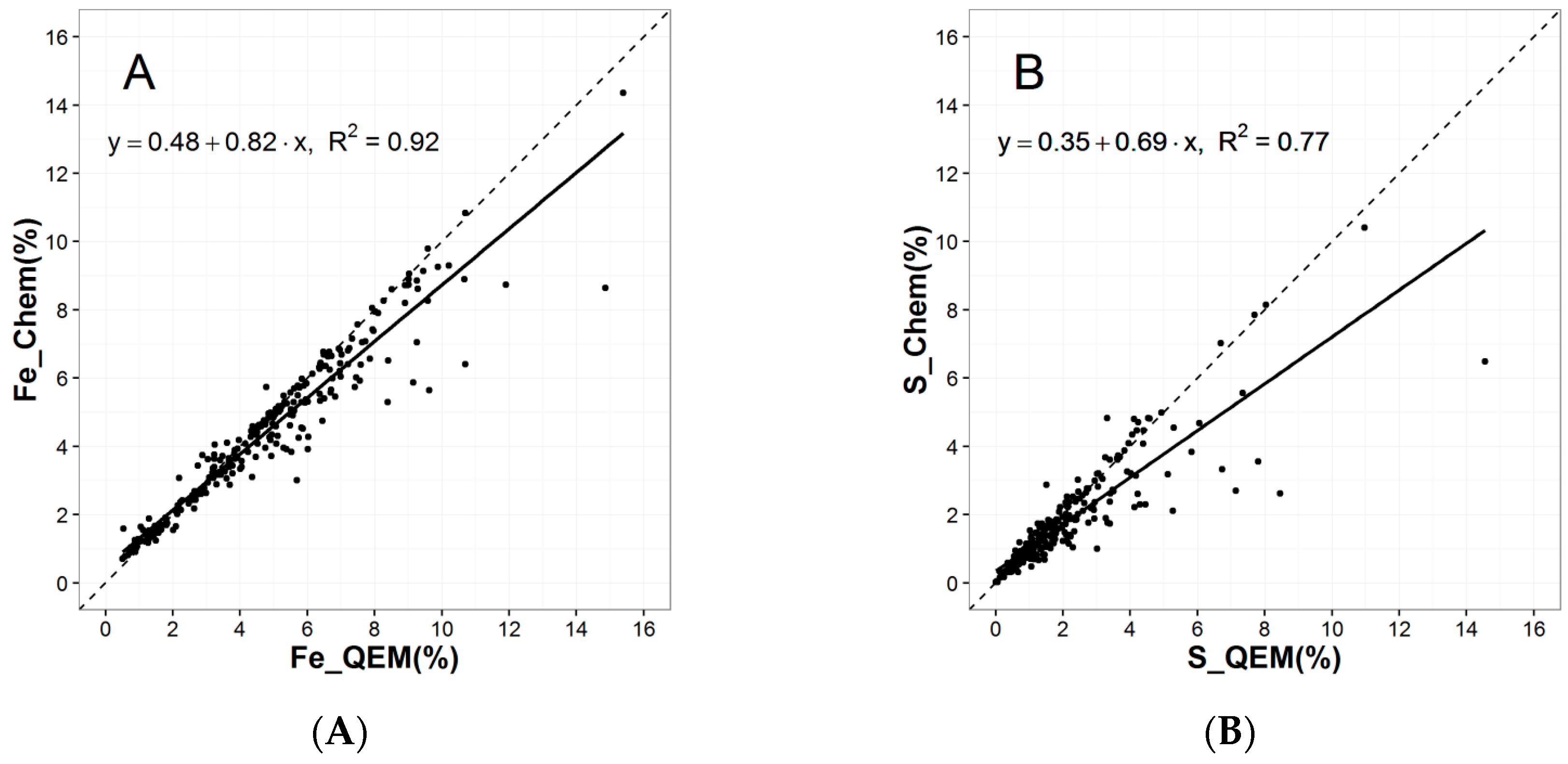
Through an extensive quality control review, significant differences were observed between results obtained by QEMSCAN® and results of elemental analyses for iron and sulfur done by atomic absorption spectroscopy (full digestion using HF, HClO4, HNO3 and HCl) and the LECO combustion furnace with infrared spectroscopy, respectively. Particularly, biases were observed which suggested that QEMSCAN® could be overestimating the weight percentages of pyrite in the samples. Figure 1 presents conciliation scatter plots for Fe and S, respectively. In the plots, the chemical assays are compared to the percentages of elements determined from QEMSCAN® results, which are calculated using the percentages of the iron- and sulfur-bearing minerals in the samples. This is commonly used as the main validation and quality control mechanism for automated mineralogical analysis [25,26,27,28]. For this conciliation, standard “textbook” compositions were used for the main sulfide minerals in the QEMSCAN® database. However, for the main iron-bearing gangue minerals (biotite, chlorite, siderite, and, to a lesser degree, tourmaline), compositions were determined through a scanning electron microscopy (SEM-EDS) study on representative mineral grains in the samples.
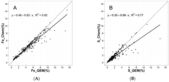
Figure 1.
Scatter plots comparing chemical assays for Fe (A) and S (B) versus percentages calculated using QEMSCAN® mineralogy. The assays were done by atomic absorption spectroscopy and LECO® (LECO Corporation, Saint Joseph, MI, USA) for Fe and S, respectively. Dotted lines represent the 1:1 correlation line, whereas solid lines are linear regression fits.
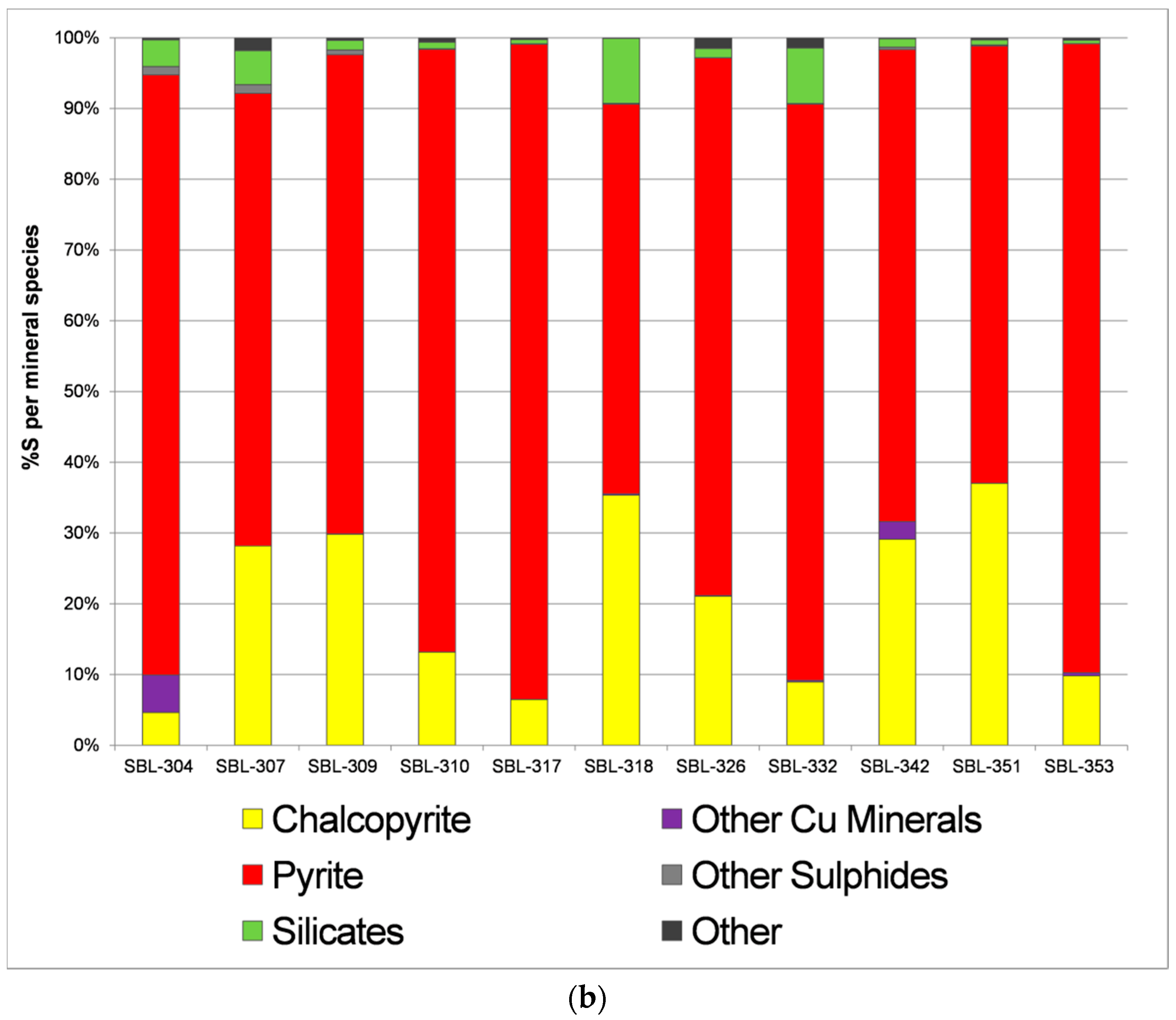
The conciliations take into account all Fe- and S-bearing species detected in the samples. However, as pyrite is among the most predominant sulfur- and iron-bearing minerals in the samples (Figure 2), the observed biases show that QEMSCAN® may be overestimating the content of this mineral.
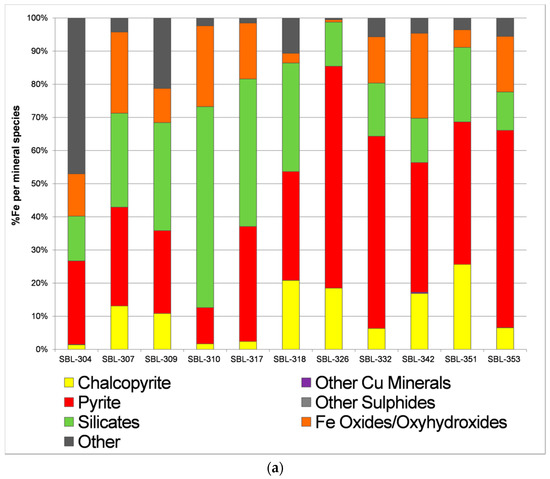

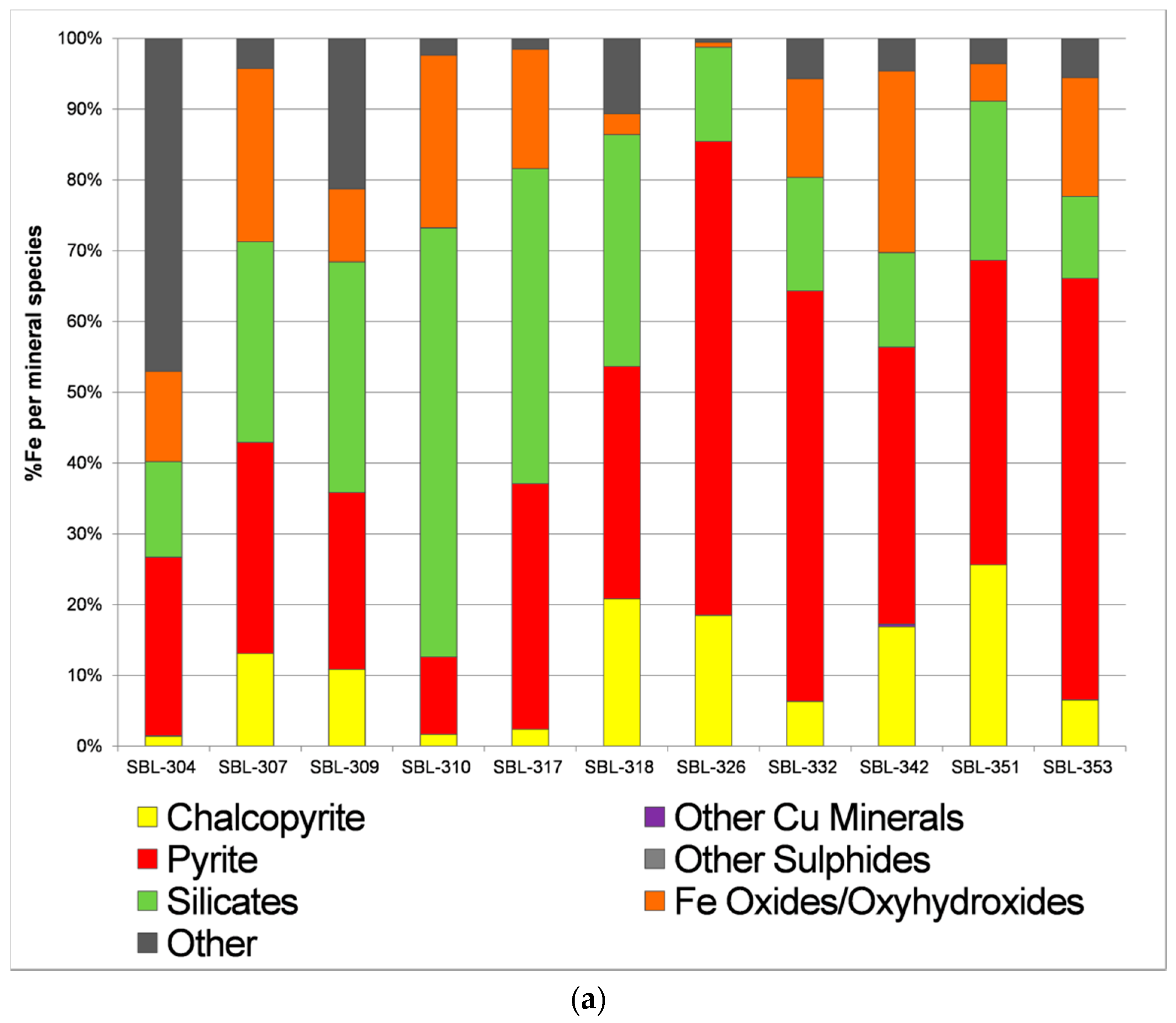
Figure 2.
(a) QEMSCAN® Elemental deportment charts for Fe and (b) S for 10 randomly chosen samples. Sulfur percentage in particular is strongly associated with pyrite in the samples.
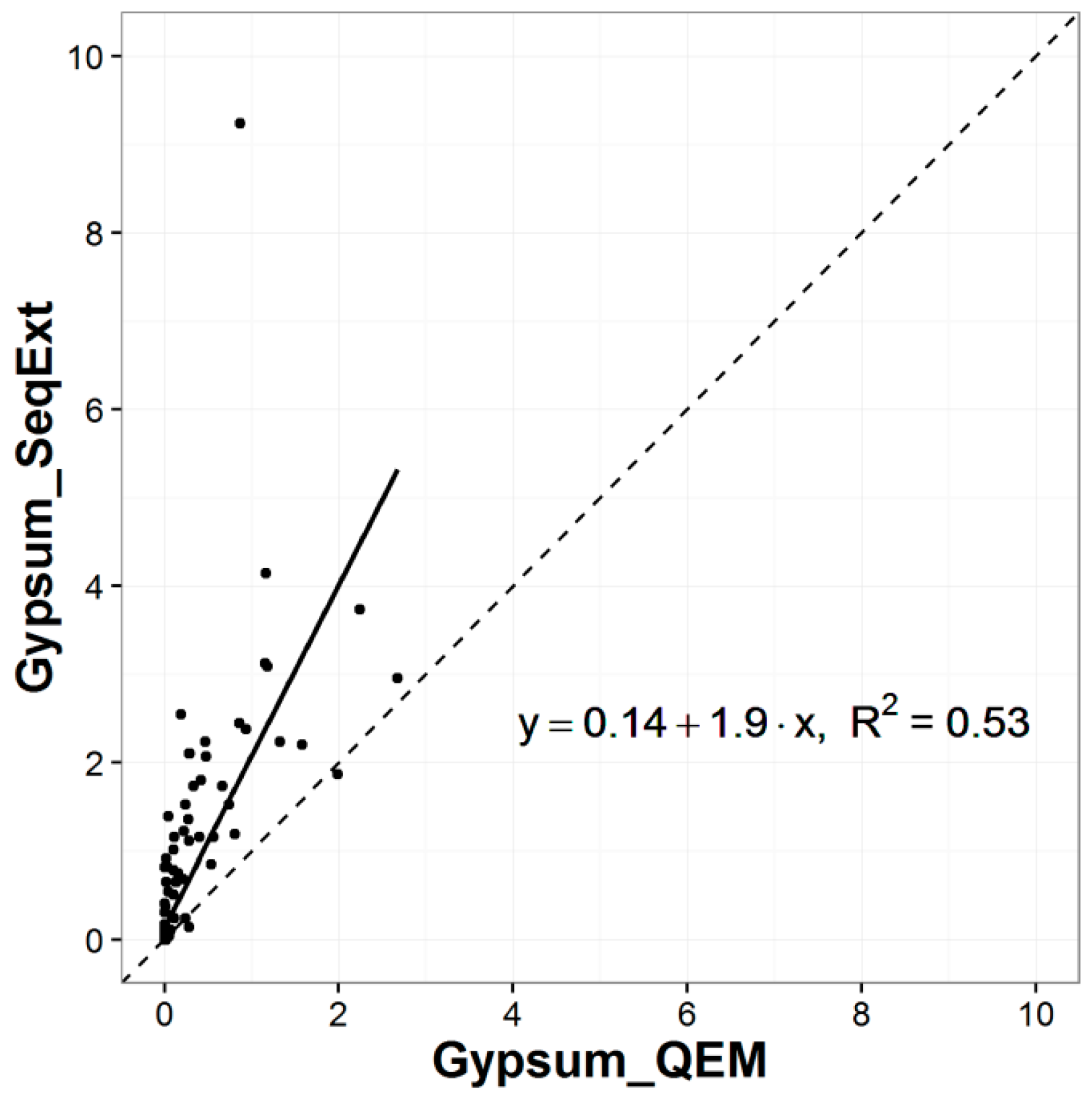
Additionally, a comparison of the mineralogical results with the sequential extraction and chemical assay data suggested that the calcium sulfate minerals may not have been adequately detected and quantified by QEMSCAN®. In general, the sequential extraction results indicated greater amounts of these minerals in the samples than the quantities detected in the QEMSCAN® analyses (Figure 3). The percentages of gypsum by sequential extraction are calculated using assays performed on the leach solution of the first step on the analysis, which is a simple partial dissolution of the pulverized sample in water at room temperature (Table 1). Therefore, the calcium assays obtained for the solution can be used to calculate the equivalent percentages of calcium sulfate, assumed to be gypsum at the time of calculation. To evaluate the validity of this comparison, the sample with the highest percentage of calcium sulfate as determined by sequential extraction was analyzed by semi-quantitative X-Ray Diffraction (XRD) using the Rietveld method. The original QEMSCAN® analysis detected 2.6% of calcium sulfate in the sample, whereas sequential extraction indicated approximately 9.2%. In order to compare the XRD results with the other techniques, the calcium sulfate minerals must be mathematically summed and considered as a group, as they cannot be individually differentiated by QEMSCAN® or the sequential extraction technique used. When summing the percentages of gypsum, anhydrite and bassanite, the XRD results indicate approximately 14.6% of calcium sulfate minerals in the sample. This result, in conjunction with the relatively high Ca assay value for the sample (3.28%), supports the hypothesis that the sequential extraction calcium sulfate percentage should be more accurate than the percentage detected by QEMSCAN® for this sample.
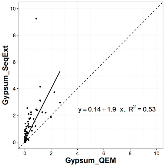
Figure 3.
Scatter plot for percentages of gypsum calculated from sequential extraction results versus those detected by QEMSCAN® analyses for 2008 study. The dotted line represents the 1:1 correlation line, whereas the solid line is the regression fit.
1.1.2. Deposit Geology and Mineralogy
The CODELCO Andina Division owns and runs the mining operations at the Rio Blanco deposit. The deposit is located approximately 70 km NNE of the Chilean capital Santiago on the western side of the Andean cordillera. Together with the adjacent Los Bronces mine, the district is classified as a “behemothian” (sensu Clark [29]) porphyry copper system [30].
The deposit is hosted within the San Francisco batholith, a large, partially-exposed quartz monzonite/quartz monzodiorite intrusion. The batholith is believed to be of early or middle Miocene age [31,32,33]. A roughly oval-shaped porphyry copper system has developed within the San Francisco batholith, which displays the typical zonations in terms of alteration types that have been recognized by previous researchers to be associated with porphyry copper deposits: a core region with potassic alteration surrounded by adjacent phyllic alteration and an extensive gradational outer halo of propylitic alteration [34,35,36]. A series of younger hydrothermal tourmaline breccias were emplaced, which host a significant proportion of the copper sulfide mineralization. Serrano et al. [37] estimated that approximately half of the copper mineralization in the Rio Blanco deposit occurs within the tourmaline-rich hydrothermal breccias, with the other half occurring in other types of breccias and as stockworks and disseminated textures in other rock types.
The common gangue and ore minerals found in the Rio Blanco deposit are summarized in Table 2 below. The main copper sulfide minerals are chalcopyrite and bornite. Secondary copper sulfide minerals, (e.g., chalcocite/digenite and covellite) are only observed locally, but can contribute substantially to the copper grades in certain zones of the deposit [37].
Table 2.
Common minerals observed in the Codelco Andina mine.
2. Methods
2.1. Mineralogical Analyses by QEMSCAN®
The QEMSCAN® instrument is an automated SEM-based mineralogical analyzer that was principally developed by the Commonwealth Scientific and Industrial Research Organisation of Australia (CSIRO) and was first presented as the “QEM SEM” at the International Mineral Processing Conference of 1982 by Miller et al. [38]. An excellent summary of the modes of mineralogical analysis available through QEMSCAN® technology can be found in Gottlieb et al. [39].
The QEMSCAN® Species Identification Protocol (SIP), which is used to identify measured energy dispersive spectra (EDS) against a “standard” mineral library for the deposit, had been previously developed by SGS Minerals Chile and validated by CODELCO Andina geologists by optical microscopy using polished thin sections. Several EDS spectra were collected for each of the minerals and SIP entries were created. A procedure similar to that described by Haberlah et al. [40] was used.
The samples that were analyzed were provided to the laboratory with a relatively coarse particle distribution size. This presented a challenge, in that the standard 3 cm diameter polished sections prepared with these particles using the traditional methodology of Jackson et al. [41] contained very high sample areas to scan, making traditional Bulk Mineralogical and Particle Mineral Analyses (BMA and PMA, respectively) by QEMSCAN® extremely slow and uneconomical for a commercial laboratory. In light of this problem, a “coarse PMA” analysis was used. Typically, the spacing between points in a PMA analysis for finer particles is in the range of 2 to 5 µm, depending on the size fraction analyzed and scale of relevant textures to be characterized, however, in the case of the coarse PMA’s performed in the Andina samples, a 15 µm step size between analysis points was used in order to reduce analysis times. Through an internal study in which several variations in modes of analysis and parameters were tested, it was determined that the coarse PMA analysis with a 15 µm step size was the best compromise between analysis time and quality of data generated.
In the current study, however, the only objective for the automated mineralogical analyses was the determination of bulk modal composition. Therefore, the particle sizes could be reduced and a more traditional approach to sample preparation and analysis could be evaluated. Given the aforementioned flexibility and the problems previously encountered with the large particle sizes, sample preparation tests which included mechanical particle size reduction were undertaken (Table 3) and the Bulk Mineralogical Analysis (BMA) QEMSCAN® mode was used. The following variations of polished section preparation methods used:
- Tests 1 to 3: Evaluate effect of sieving the samples into several particle size fractions. More replicates are analyzed for the coarser fractions, because in these cases fewer particles are exposed at the surface of each 3 cm diameter polished section. The number of sections and size fractions are systematically reduced from Tests 1 to 3 in order to observe the effect on overall results.
- Test 4: The sample is not divided into size fractions, but a duplicate polished section is analyzed in order to evaluate the effect of increasing the number of particles with respect to the original analyses.
- Test 5: The use of transverse sections is investigated, where the original section is cut vertically and the two halves generated are turned 90° and mounted in a new resin-encapsulated polished section, exposing the vertical profile of the original section. It is hypothesized that this may reduce or eliminate the effect of particle segregation in the original section (e.g., Kwitko-Ribeiro [42]; Blaskovich [16]; Grant et al. [43]).
- Test 6A and 6B: The effect of particle size reduction through controlled mechanical pulverization is evaluated. The objective is to reduce the range of particle sizes and therefore the competition between particles as they settle towards the bottom of the sample mold during resin curing.
Table 3.
Sample preparation scheme for particle and mineral segregation study.
For the investigation of a sample preparation method which would preserve calcium sulfate minerals in the polished sections, ethylene glycol was used instead of water as a polishing lubricant during the lapping process.
For the purpose of elemental conciliation and quality control, chemical assays for Cu, Fe and S were performed on the head samples using the same methods described previously in Section 1.1.1.
2.2. Sequential Extraction Analyses
The method for the sequential extraction analyses used in this study is that which was published by Dold [24]. Similar procedures, which aim to detect the trace elements associated with specific groups of minerals, have been developed in the past, notably beginning with the methodology published by Tessier et al. [44] for river sediments. However, the seven step variation developed by Dold [24] was designed to increase the selectivity in the dissolution of iron oxides and oxyhydroxides and was tailored to the specific primary and secondary mineralogy of porphyry copper systems. As these minerals play significant roles in trace element mobility and retention in mine waste environments, this method was chosen for the environmental study. Details of the procedure can be found in Table 1.
3. Results and Discussion
3.1. Mineralogical Analyses
3.1.1. Particle Segregation Study
In order to confirm the presence of particle segregation and evaluate the degree to which it was occurring in the previously analyzed polished sections, one of the sections was selected for vertical slicing and preparation of a transversely-mounted polished section. The sample selected was one for which QEMSCAN® detected considerably higher proportions of Fe and S in relation to the chemical assays. The transverse section was prepared and analyzed by the Field Scan mode. This analysis mode generates a full mineral map of the exposed surface of the polished section. It is evident that a very high degree of particle segregation is present in the section (Figure 4). Particle masses have been calculated using the mineralogical results and the respective densities and extrapolated volumes of each mineral species. It can be seen that the particles with greater mass are concentrated near the center of the section, which represents the bottom of the original polished section (the zone in which the particles would sink to during the resin curing process), which was the original analysis surface. Note the high proportion of sulfide (mainly pyrite) grains in this zone, due to the higher density of pyrite (4.95–5.03 g/cm3; Deer et al. [45], in relation to the silicate gangue mineralogy (~2–3 g/cm3).
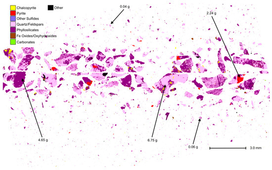
Figure 4.
Mineral map produced for a Field Scan analysis of an entire transverse section surface. Particle segregation is clearly evident. Arrows indicate the mineralogically calculated particle masses for the entire particle that they point to. Note the concentration of heavier, sulfide-rich particles towards the center of the transverse section, which represents the bottom of the original section.
Having confirmed the existence of a particle segregation problem, the different varieties of polished sections were prepared carefully. Any polished sections that were found to display scratches, relief, holes/bubbles in the hardened resin, or particles damaged by the polishing process were discarded and prepared again until satisfactory results were achieved. The accepted polished sections were analyzed using the BMA analysis mode.
In order to evaluate the degree of segregation of pyrite in the samples, the chemical assays for Fe and S were used. In addition to the elemental deportment data presented in Figure 2, which shows that pyrite hosts a significant proportion of these elements in the samples, a correlation analysis also detected strong, statistically significant positive linear correlations between these elements and pyrite percentage in the previously analyzed samples. The correlation between sulfur and pyrite for these samples is especially strong (R2 = 0.863) (Table 4). Therefore, a good conciliation between sulfur and iron chemical assays and the percentages of these elements calculated from the mineralogical results would suggest that the quantities of pyrite determined by QEMSCAN® should be accurate.
Table 4.
Correlation table for pyrite with Fe and S chemical assays. A very strong and statistically significant correlation is identified between pyrite and S.
Initially, three samples were selected to test each method of polished section preparation. The conciliation between the chemical assays and mineralogically calculated results for Fe, Cu, and S were studied in order to evaluate each section preparation method in terms of the degree of associated sulfide segregation. The error was calculated as follows:
where:
%Relative Error= (%Element_QS − %Element_Chem)/(%Element_Chem) × 100
- %Element_QS = The calculated elemental percentage based upon QEMSCAN® mineralogical results.
- %Element_Chem = The measured elemental percentage from traditional chemical assays.
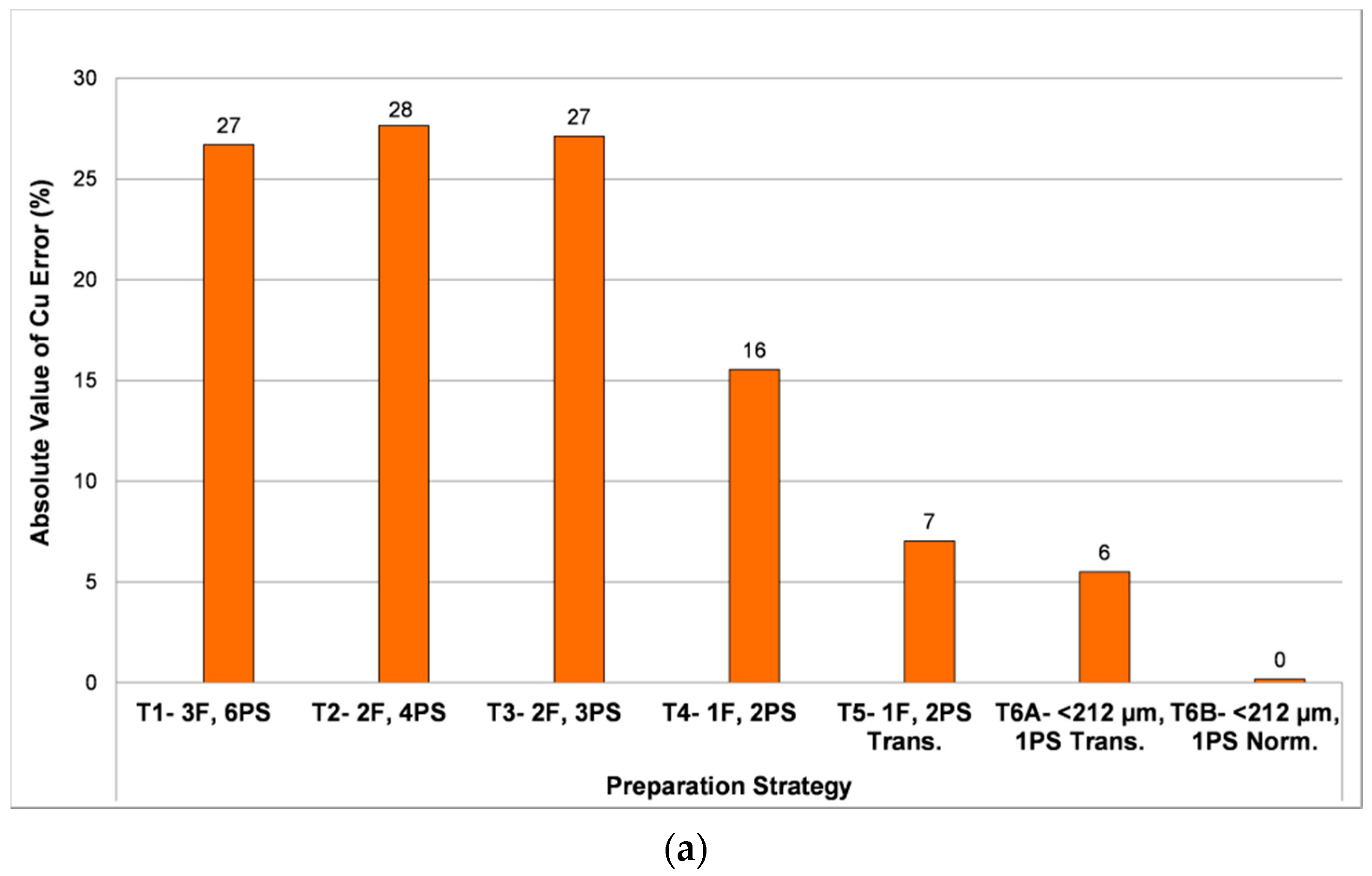
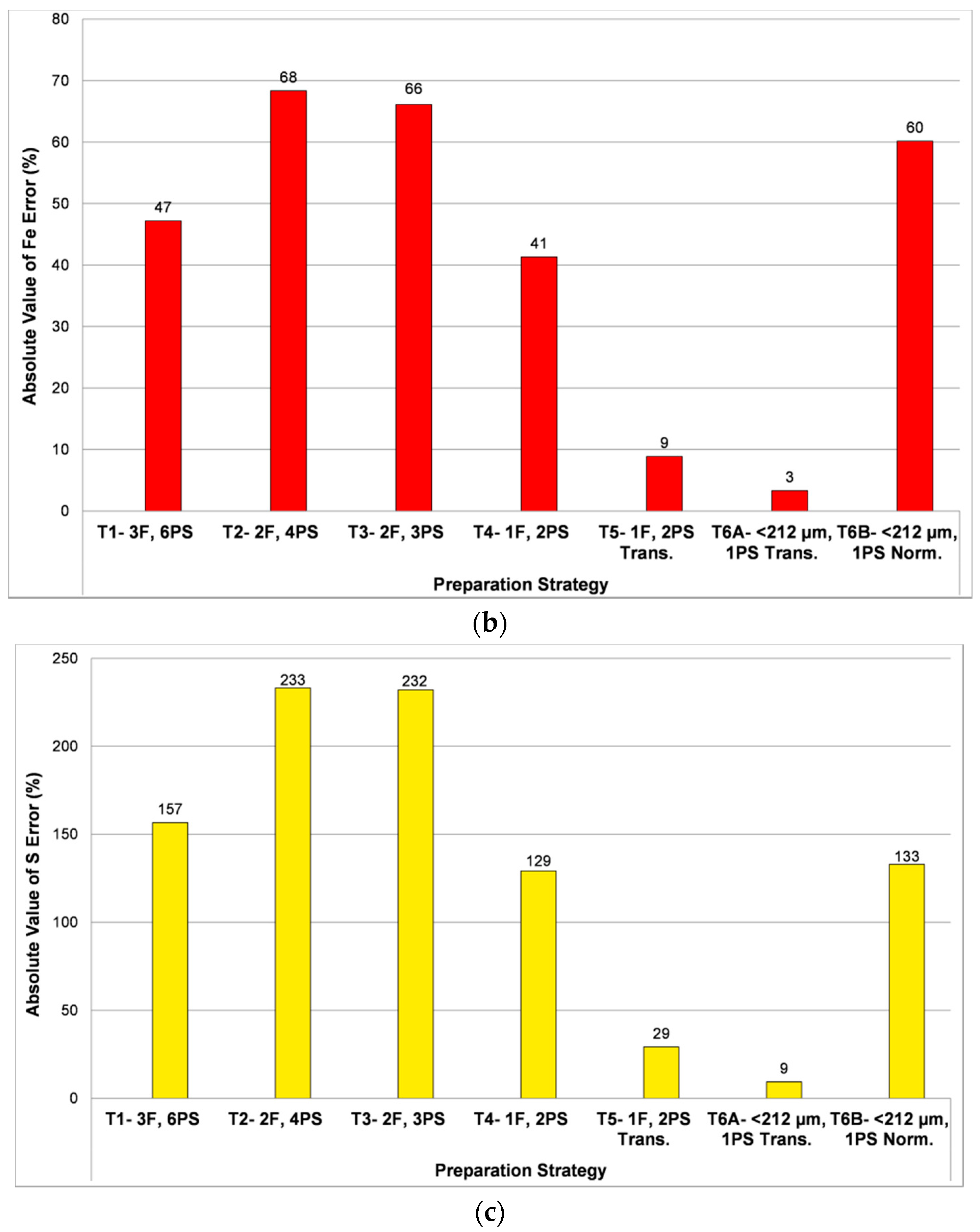
Copper was included in order to ensure a high accuracy in the characterization of copper sulfide minerals. Figure 5 presents the results of the errors obtained for this comparison for each of the polished section preparation methods. The charts indicate that Tests 1 through 3 (T1–T3), in which the samples are divided into size fractions and replicate polished sections are produced for the coarser particle sizes, generally illustrate higher percentages of error (~27% for Cu, ~61% for Fe, and ~207% for S) in the conciliation of chemical elements. The conciliation for sulfur is associated with the highest errors, followed by iron and finally copper. Tests 2 (two size fractions, four total polished sections) and 3 (two size fractions, three total polished sections) were particularly ineffective in reducing pyrite segregation, with errors greater than 60% for iron and in the range of 230% for sulfur. Test 4, which used two polished sections and the original particle size distribution with no granulometric separation, returned errors in an intermediate range with the error for iron being ~41% and that of sulfur ~129%. The charts in Figure 5 illustrate that clearly, for the three samples tested, the transverse polished sections provided the results with the lowest average errors for the elemental conciliations. The conciliations for T6A present the lowest average errors for all three elements. This test involves a particle size reduction to 100% <212 µm, followed by the preparation and analysis of a single transverse section for each sample. This methodology was associated with low conciliation errors for Fe and S, the two elements which comprise pyrite (FeS2). The conciliation error for copper was lowest for Test 6B, which involved particle size reduction as in Test 6A, but a traditional (not transverse) resin-encapsulated polished section was prepared with the resulting material. Although a very low error was calculated for Cu using this methodology, the Fe and S errors were relatively high (~60% and ~133%, respectively).

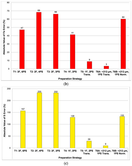
Figure 5.
Average errors for (a) Cu; (b) Fe and (c) S calculated by calculating the difference between the QEMSCAN® results for each of the sample preparation tests vs. chemical assays, and then computing the average for all three samples. T1: three size fractions with a total of six polished sections; T2: two size fractions with a total of four polished sections; T3: two size fractions with a total of three polished sections; T4: no size division, original and duplicate polished sections prepared; T5: no size division, two transverse polished sections prepared; T6A: granulometric size reduction and preparation of one transverse polished section; T6B: granulometric size reduction and preparation of one traditional polished section.
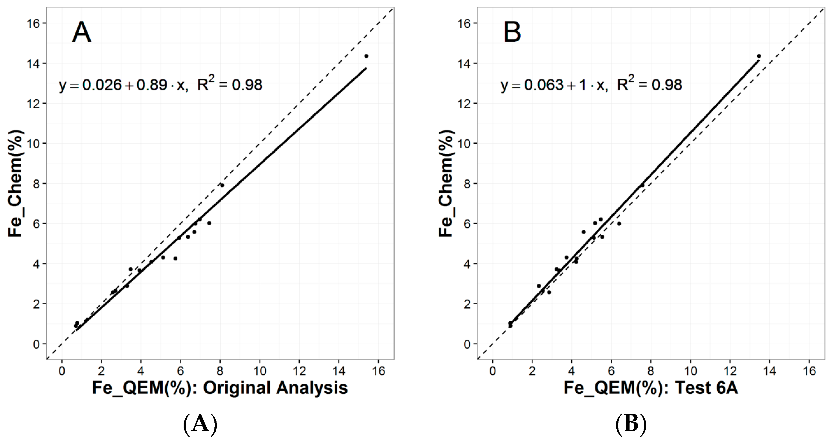
The results for the three samples tested suggest that the method with the most potential to reduce the impact of pyrite segregation while also providing accurate results for copper sulfides and other minerals was that which was used for Test 6A (particle size reduction to <212 µm and preparation of one transverse section per sample). A validation study was carried out using 15 additional samples which had presented problems of pyrite segregation in their original analyses. All polished sections were prepared using the methodology of Test 6A and ethylene glycol as a polishing lubricant. In the case of iron, although the conciliations are similar in terms of R2 value, there is a greater bias in the results for the 18 samples analyzed in the previous study towards higher Fe values in the QEMSCAN® results. Using the new polished section preparation methodology, this bias is not observed and values display a more random distribution around the 1:1 correlation line (Figure 6).
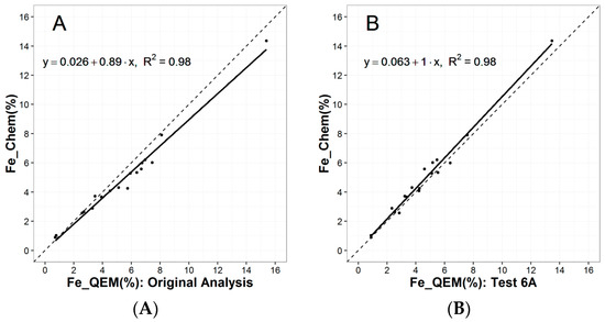
Figure 6.
(A) Elemental conciliations for Fe for eighteen samples, comparing QEMSCAN® results vs. chemical assays by atomic absorption spectroscopy for the original QEMSCAN® results from 2008 and (B) the results obtained for the polished section prepared using the methodology from Test 6A, which involved sample particle size reduction and preparation of a transverse polished section.
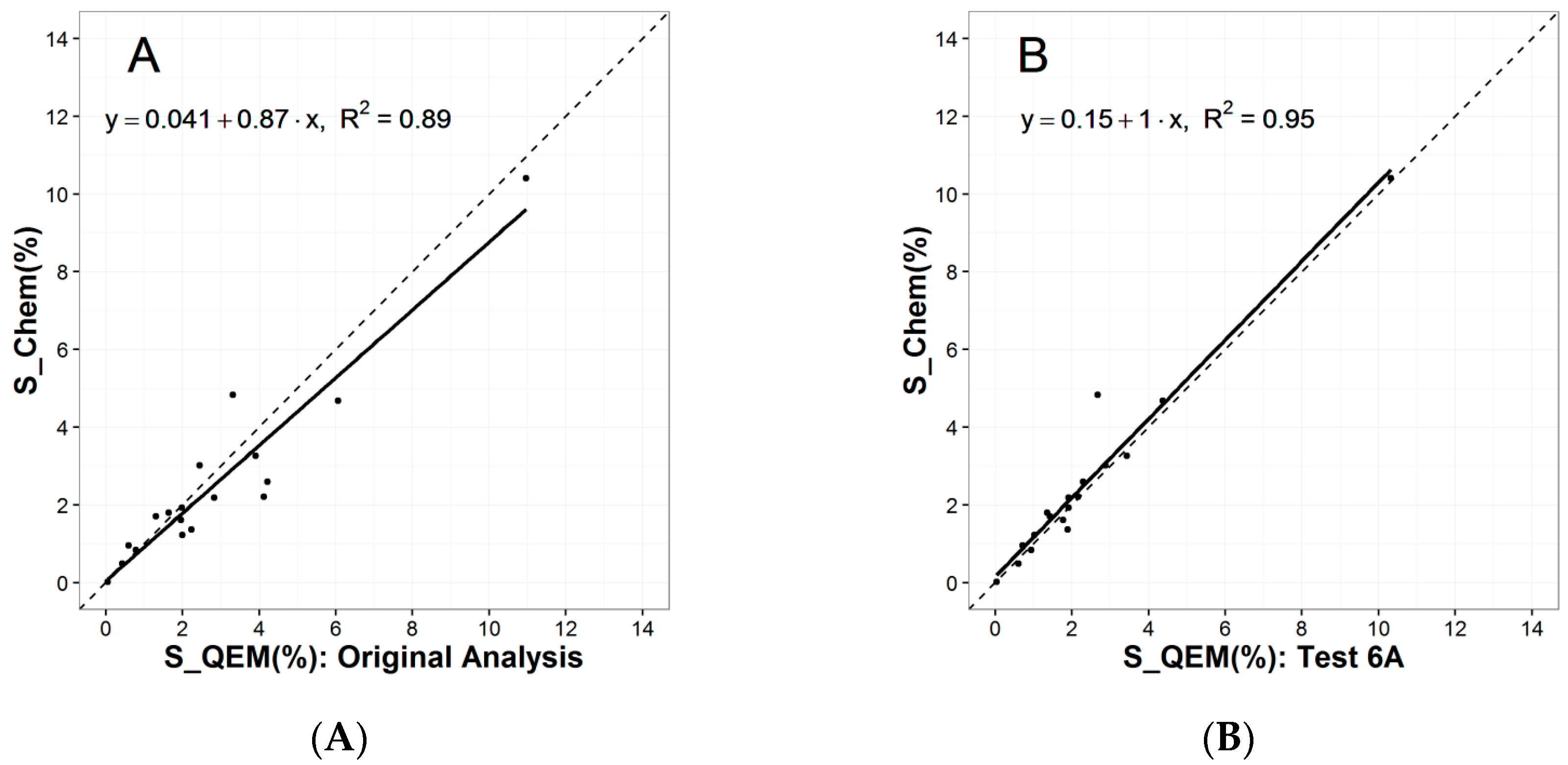
The sulfur correlation also displays a bias towards higher values for the QEMSCAN® results in relation to the chemical assays for the polished sections used in the original study (Figure 7). Results indicate a marked improvement using the particle size reduction and transverse section methodology, where values are much closer to a 1:1 correlation between chemical assays and QEMSCAN® elemental calculations. There is a clearly identifiable outlier in Figure 7B for which the sulfur percentage determined by chemical assay is much higher than that which was calculated using the mineralogical results. This point represents sample SBL-313, for which the sequential extraction results indicate a high percentage of water-soluble calcium sulfate minerals (~9%). Therefore, it is probable that during the polishing process there was dissolution of these minerals and a loss of sulfur occurred. This means that the differences in sulfur percentages are very likely related to the loss of calcium sulfates and not to pyrite.
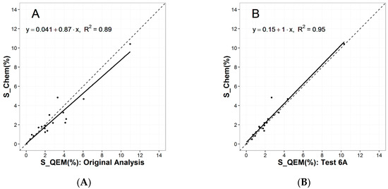
Figure 7.
(A) Elemental conciliations for S for eighteen samples, comparing QEMSCAN® results vs. chemical assays by atomic absorption spectroscopy for the original QEMSCAN® results from 2008 and (B) the results obtained for the polished section prepared using the methodology from Test 6A, which involved sample particle size reduction and preparation of a transverse polished section.
As an additional validation, the percentages of pyrite from the QEMSCAN® analyses were compared to those which were calculated from the sequential extraction results for step 6 of the procedure (Figure 8). Note that the sequential extraction pyrite values should be considered semi-quantitative and can only be used as an approximate value. For sequential extraction, the sulfide minerals proportions are calculated through the use of previous qualitative knowledge of the sulfide minerals in the sample which would contribute to the concentrations of certain elements in the solution obtained after the oxidation/dissolution reactions that occur in step 6. The sequence of calculations for the Codelco Andina samples using the assay results obtained for the solution extracted in step 6 is detailed below. Note that steps 1 through 3 in the calculation assume that the specified element was extracted only from the specified mineral. Also, it should be noted that the concentrations of elements in tennantite were determined by electron probe microanalysis (EPMA). For all other minerals, standard textbook compositions were used for the calculations.
- Calculate %galena (using %Pb from the chemical assay)
- Calculate %molybdenite (using %Mo)
- Calculate %tennantite (using %As)
- Calculate %sphalerite (%Zn_total − %Zn_tennantite)
- Calculate %chalcopyrite (%Cu_total − %Cu_tennantite)
- Calculate %pyrite (%S_total − %S in the minerals from 1 to 5 above)
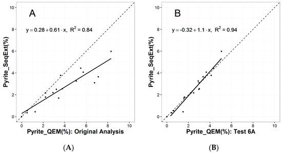
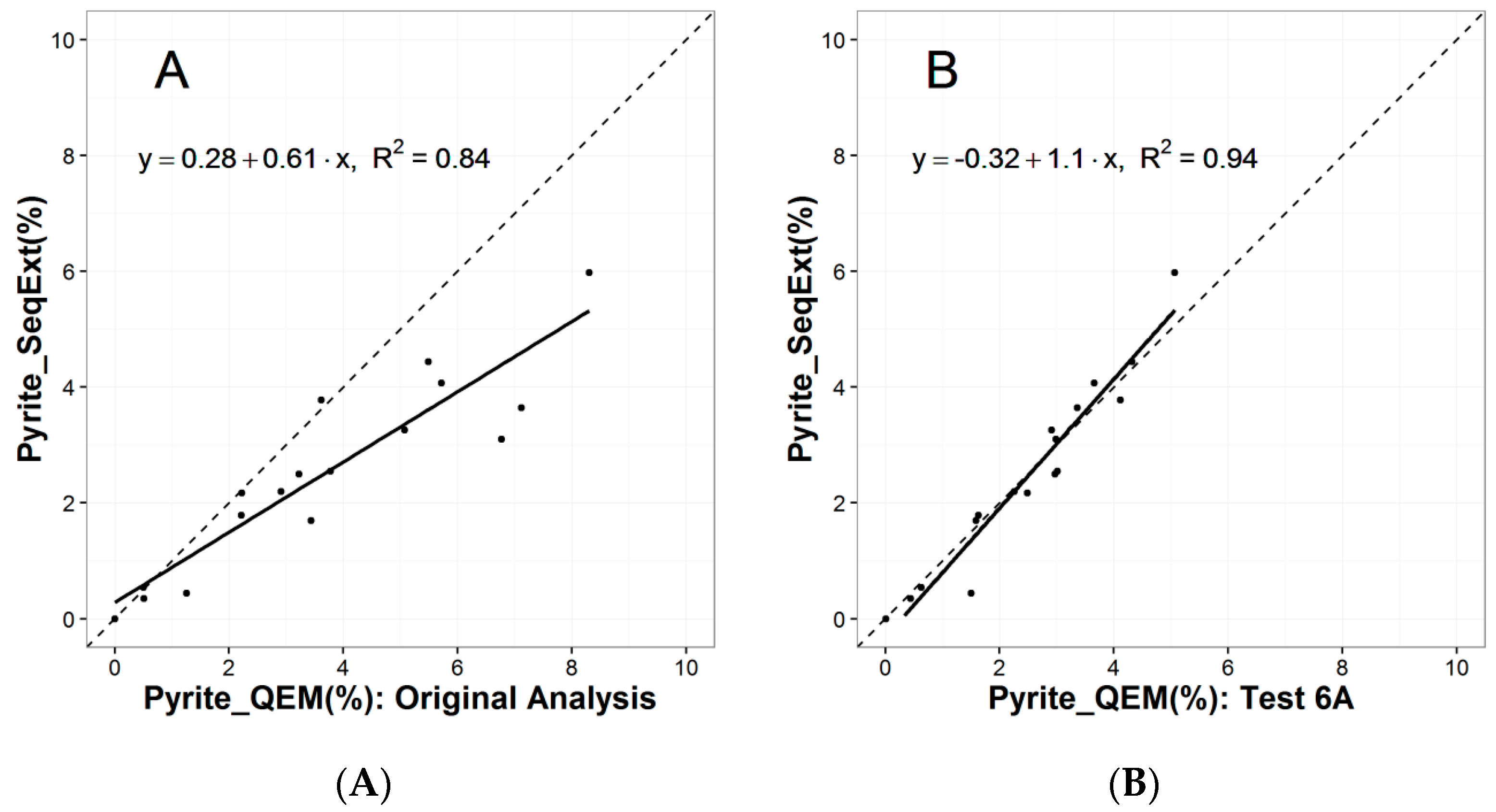
Figure 8.
(A) Conciliation for pyrite using eighteen samples. Comparison is for pyrite percentages calculated with sequential extraction results vs. the original QEMSCAN® results from 2008 and (B) the results obtained for the polished section prepared using the methodology from Test 6A, which involved sample particle size reduction and preparation of a transverse polished section.
The results illustrate an acceptable degree of conciliation between the percentages of pyrite detected by QEMSCAN® using the new polished section preparation methodology and the values calculated from the sequential extraction results. The same comparison, when realized using the QEMSCAN® results from the previous study shows a poorer and more biased conciliation.
The density segregation phenomenon is relatively common in polished sections made for encapsulated particles of sulfide and other dense mineral ores and their metallurgical processing wastes. Mermillod-Blondin et al. [46] developed mathematical corrections for automated mineralogical results generated from hardened epoxy sections with the objective of reducing the impact of the segregation effect. However, the validity of using Stoke’s law, in which particles are assumed to be smooth and spherical and the material homogeneous, to account for the phenomenon is questionable. Porphyry copper samples typically deviate strongly from this assumption, often showing predominant phyllic alteration and high quantities of tabular-shaped fine mica particles. In this case, the most effective and simple solution to the problem would be to control the phenomenon during the sample preparation process, or to develop modifications to sample mounting before analysis to mitigate the effect on mineral quantification ([16,28,42], this study).
The methodology proposed in this study, in which particle sizes were first reduced and transverse section mounts were prepared, shows the best results thus far. This is probably in part due to increased homogeneity in particle size and mass, which would likely reduce vertical segregation in the original polished section. Also, the particle size reduction gave way to the accommodation of a larger number of individual particles in the exposed vertical section (~90,000 particles) when compared to a transverse section that was prepared for the same sample, but with the original (coarser) particle size distribution (~12,000 particles). According to particle sampling theory, if each particle analyzed is considered as a sampling increment, the section containing 90,000 particles should be more representative than that which contained 12,000 particles [47,48]. An inadequate number of particles may also explain the poor results observed in sample preparation Tests 1 through 4, which used coarser particles.
While this sample preparation methodology may offer a feasible solution for studies in which the only objective is the determination of mineralogical composition, this would not be suitable for studies in which spatial relationships and textures are to be conserved and characterized. In a hypothetical case where composition and sulfide grain exposure are to be evaluated, an effective procedure may be to determine the bulk mineralogical composition using the methodology described in this study. Then, a “traditional” polished section, where vertical segregation has not been compensated for, may be prepared for the sole purpose of sulfide liberation, exposure and textural characterization, using the Specific Mineral Search (SMS) or Trace Mineral Search (TMS) modes of analysis, depending on the range of expected target mineral concentration [49]. A traditional polished section with sulfide segregation would favor these types of analysis, where it is important to characterize the greatest number of target mineral grains per polished section in order to increase statistical robustness [28].
3.1.2. Particle Number Determination
In order to determine an adequate analysis time, which would be neither excessive nor insufficient and that would ensure a reasonable analytical precision, a study was carried out to evaluate the impact that the number of points analyzed by the QEMSCAN® BMA mode has on the mineralogical results.
An excessively long BMA analysis was performed for 18 samples in order to obtain a very large number of particle intercepts for each of them, generating a representative and statistically robust mineralogical composition for the sample surface. Subsets of randomly chosen particles were selected at interval steps of 10%, starting at 90% and finishing at 10% of the total population of measured particles. For each subset, the calculated mineralogical composition was saved. The minerals were binned by their percentages and comparisons were made between the percentage of each mineral in each of the subsets and the percentage of the same mineral in the robust analysis (i.e., considering the full population of measured particles). The mineral percentage groups used in each of the subsets are as follows:
- >0% < 1%
- ≥1% < 5%
- ≥5% < 12%
- ≥12%
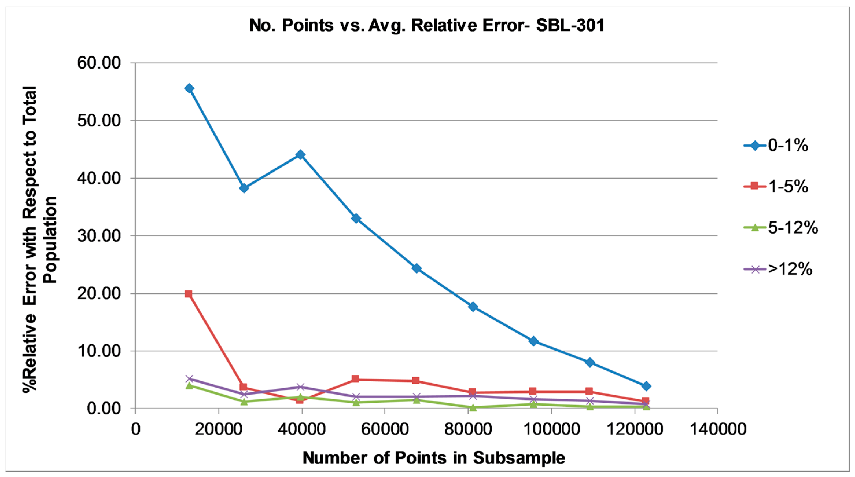
Given that the number of particles and analysis points demonstrate a perfect linear correlation (R2 = 1.00), the number of analysis points in each subset was plotted against the average relative difference for each of the four mineral percentage ranges for each of the subsets (10% of total particles, then 20%, 30%, etc.). Figure 9 shows an example of this exercise for sample SBL-301.
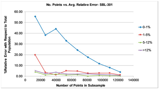
Figure 9.
Chart illustrating the effect of the number of analysis points on the repeatability of mineralogical results for minerals present in the percent ranges illustrated in the legend for sample SBL-301. In this case, ~101,000 points are required in order to achieve a relative error of <10% for all of the four mineral modal percent ranges.
It was determined that a relative difference of <10% for all mineral ranges was an acceptable goal. The data suggest that for minerals which occur in percentages of >1 wt% in the samples, it was necessary to analyze approximately 50,000 points in order to ensure a precision of <10% with respect to an extensive analysis of more than 100,000 points. However, for mineral species present in proportions <1% an analysis of approximately 120,000 points was necessary to ensure the same degree of precision. Therefore, it was determined that future BMA analyses of the polished sections prepared for Andina samples using the proposed methodology should be performed with parameter settings that aim to obtain 120,000 points as a minimum.
3.1.3. Ethylene Glycol Polishing Tests
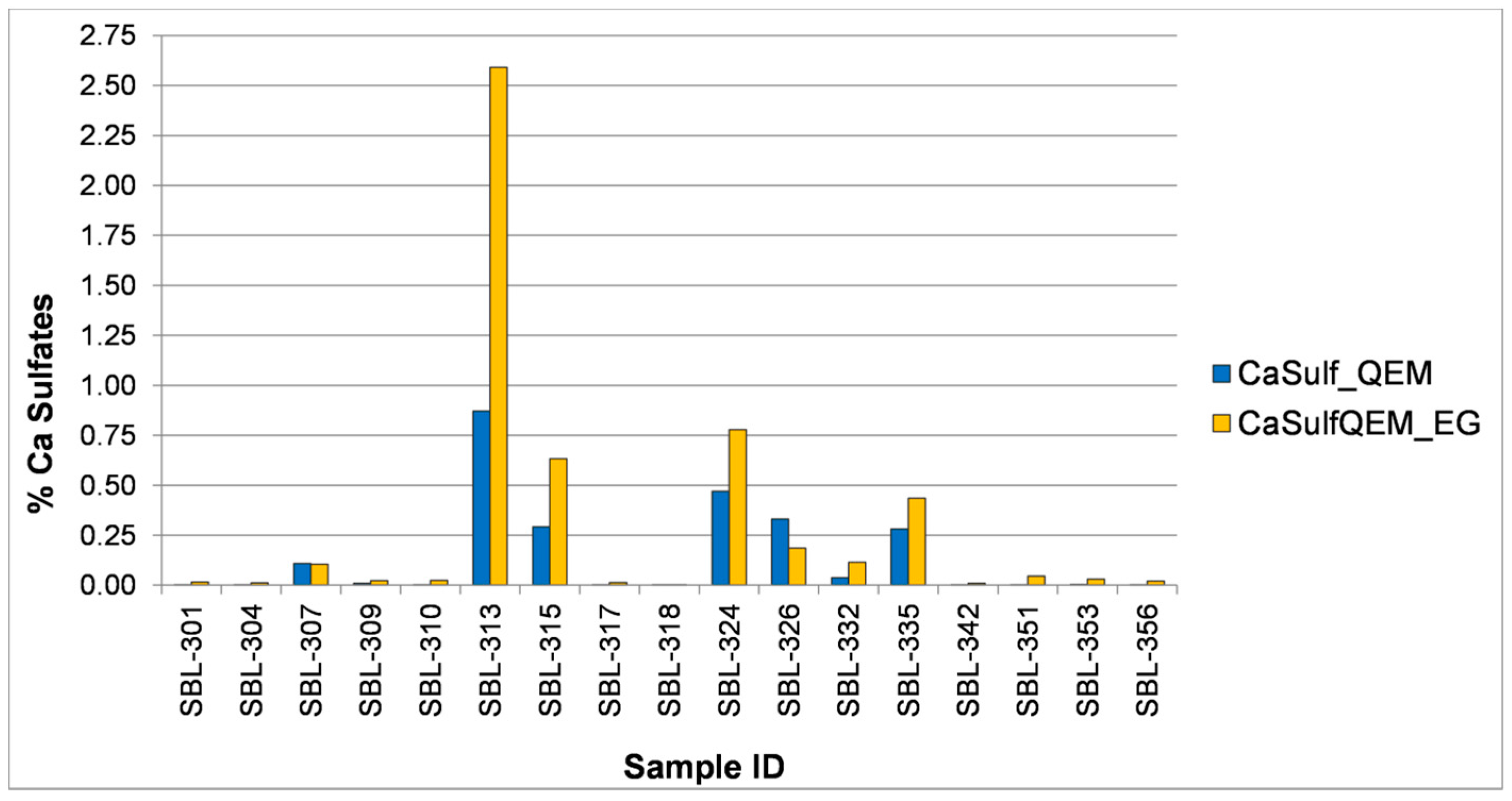
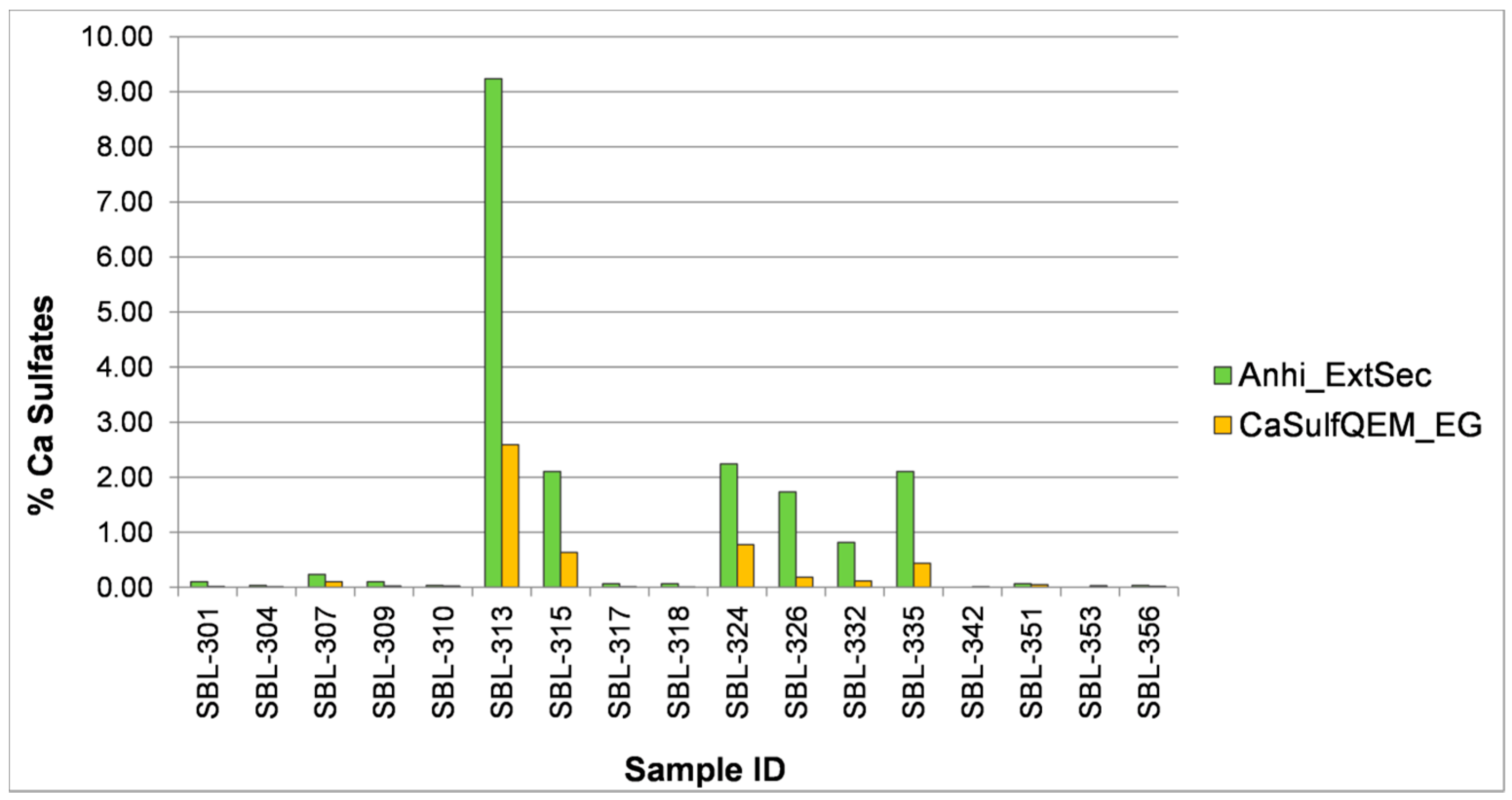
With very few exceptions, the results generally indicate a higher percentage of calcium sulfate minerals in the samples for the ethylene glycol (EG) sections than for the original water polished sections (Figure 10), using the same analytical parameters and mineral library database. However, when compared to the quantities of these minerals calculated using the chemical assays obtained after step 1 of the sequential extraction analysis, the QEMSCAN® results for Ca sulfate minerals are still generally lower (~68% lower, on average) (Figure 11).
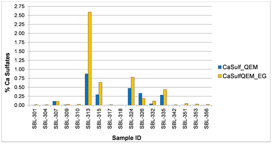
Figure 10.
Comparison of the percentages of calcium sulfate minerals detected by QEMSCAN® for sections polished with water (CaSulf_QEM) vs. ethylene glycol (CaSulfQEM_EG).

Figure 11.
Comparison of the percentages of calcium sulfate minerals calculated with sequential extraction results (Anhi_ExtSec) vs. detected by QEMSCAN® for the ethylene glycol polished sections (CaSulfQEM_EG).
Improvements were observed in the conciliation between the percentages of calcium sulfate minerals calculated from sequential extraction results and those detected by QEMSCAN® analyses with the use of ethylene glycol as a polishing lubricant instead of water. However, the relative differences between the percentages of these minerals determined by the two techniques were still considered to be large and unacceptable. The sum of sequential extraction Inductively Coupled Plasma Optical Emission Spectroscopy (ICP-OES) results for Ca also agree better with whole-rock calcium assays done by atomic absorption spectroscopy than with the QEMSCAN® results, which are typically lower for calcium than both analytical techniques.
Some sample preparation laboratories have experimented with kerosene and ethanol as alternative lubricants. The concrete industry has been known to use these liquids for petrographic specimen preparation to avoid the dissolution of soluble minerals (e.g., Poole and Sims [50]). These liquids were not tested in this study, as the laboratory used could not accommodate the dangers they present in terms of vapor toxicity and flammability.
Given the abundance of soluble sulfates in hydrothermal systems and waste deposits, great care must be taken to preserve these minerals during sample preparation for mineralogical analysis. In any case, further investigation into this topic is highly recommended.
4. Conclusions
A series of sample preparation tests determined that the most effective methodology for reducing the effect of particle and mineral segregation on mineralogical results for samples from the Rio Blanco porphyry copper deposit involved a particle size reduction, followed by the preparation and analysis of a transversely-mounted polished section which exposed the vertical profile of the original section. The results illustrate that pyrite is more accurately quantified by this method. The critical importance of accurate pyrite quantification in environmental mineralogy studies cannot be understated. Therefore, the use of this methodology of automated mineralogical analysis is likely appropriate and beneficial for similar studies on other ore deposit samples.
The dissolution of soluble calcium sulfates in the samples, believed to be caused by the use of water as a lubricant during the grinding and polishing of the sections, was reduced through the replacement of water by ethylene glycol. Although a positive effect in the conservation of calcium sulfate minerals was observed, the results of QEMSCAN® analyses on the polished sections prepared with ethylene glycol were still much lower than the true amounts of these minerals expected to be present in the samples, based on chemical assay data. Other industries and laboratories have indicated greater conservation of water-soluble minerals through the use of paraffin or alcohol as polishing lubricants, but these options are potentially expensive and dangerous. Therefore, a more appropriate lubricant solution for petrographic section preparation of samples containing water-soluble minerals needs to be identified.
Acknowledgments
The authors would like to express their gratitude to the staff of CODELCO, Andina Division for their support and review of this study and permission for publication. The contributions of Leyla Weibel, César Bustos, JavierCruz and Claudio Martinez are acknowledged. Additional gratitude is owed to Fernando Medina of CODELCO for valuable input. We would also like to thank Brandon Youlton of SGS Minerals, South Africa and Eduardo Ardiles of SGS Minerals Chile for their disposition and expertise with the analysis and interpretation of XRD analyses. Finally, we would like to thank Peta Hughes and Mauricio Belmar of SGS Minerals for their support of this study and generosity with QEMSCAN® instrument time.
Author Contributions
Robert Pooler and Bernhard Dold developed the methodology and experimental design for this study. Mineralogical analyses were performed by Robert Pooler. Analysis and interpretation of the results was performed by Robert Pooler and Bernhard Dold. The manuscript was written by Robert Pooler with contributions from Bernhard Dold.
Conflicts of Interest
The authors declare no conflict of interest.
References
- Price, W. Prediction Manual for Drainage Chemistry from Sulphidic Geologic Materials; Mend Report; Mining and Mineral Sciences Laboratories: Smithers, BC, Canada, 2009; pp. 1–579. [Google Scholar]
- Dold, B. Submarine tailings disposal—A review. Minerals 2014, 4, 642–666. [Google Scholar] [CrossRef]
- Smuda, J.; Dold, B.; Spangenberg, J.E.; Pfeifer, H.R. Geochemistry of fresh alkaline porphyry copper tailings: Implications on sources and mobility of elements during transport and early stages of deposition. Chem. Geol. 2008, 256, 62–76. [Google Scholar] [CrossRef]
- Dold, B.; Fontboté, L. Element cycling and secondary mineralogy in porphyry copper tailings as a function of climate, primary mineralogy, and mineral processing. J. Geochem. Explor. 2001, 74, 3–55. [Google Scholar] [CrossRef]
- Plumlee, G.S. The environmental geology of mineral deposits. In The Environmental Geochemistry of Mineral Deposits; Part A, Processes, Techniques and Health Issues; Plumlee, G.S., Logsdon, M.J., Eds.; Society of Economic Geologists: Littleton, CO, USA, 1999; pp. 71–116. [Google Scholar]
- Dold, B. Basic concepts of environmental geochemistry of sulfide mine-waste. In UNESCO-SEG-SGA Latin American Metallogency Course; Ponificia Universidad Católica del Perú: Lima, Perú, 2005; p. 36. [Google Scholar]
- Dold, B. Evolution of Acid Mine drainage formation in sulphidic mine tailings. Minerals 2014, 4, 621–641. [Google Scholar] [CrossRef]
- Dold, B.; Weibel, L. Biogeometallurgical pre-mining characterization of ore deposits: An approach to increase sustainability in the mining process. Environ. Sci. Pollut. Res. 2013, 20, 7777–7786. [Google Scholar] [CrossRef] [PubMed]
- Dold, B. Basic concepts in environmental geochemistry of mine waste management. In Waste Managemente; Kumar, S., Ed.; InTech: Rijeka, Croatia, 2010; pp. 173–198. [Google Scholar]
- Nordstrom, D.K.; Alpers, C.N. Negative pH, efflorescent mineralogy, and consequences for environmental restoration at the Iron Mountain Superfund site, California. Proc. Natl. Acad. Sci. USA 1999, 96, 3455–3462. [Google Scholar] [CrossRef] [PubMed]
- Dold, B.; Spangenberg, J.E. Sulfur speciation and stable isotope trends of water-soluble sulfates in mine tailings profiles. Environ. Sci. Technol. 2005, 39, 5650–5656. [Google Scholar] [CrossRef] [PubMed]
- Smuda, J.; Dold, B.; Spangenberg, J.E. Element cycling during the transition from alkaline to acidic environment in an active porphyry copper tailings impoundment, Chuquicamata, Chile. J. Geochem. Explor. 2014, 140, 23–40. [Google Scholar] [CrossRef]
- Nordstrom, D.K. What was the groundwater quality before mining in a mineralized region? Lessons from the Questa Project. Geosci. J. 2008, 12, 139–149. [Google Scholar] [CrossRef]
- Parbhakar-Fox, A.; Lottermoser, B.; Bradshaw, D. Evaluating waste rock mineralogy and microtexture during kinetic testing for improved acid rock drainage prediction. Miner. Eng. 2013, 52, 111–124. [Google Scholar] [CrossRef]
- Becker, M.; Dyantyi, N.; Broadhurst, J.L.; Harrison, S.T.L.; Franzidis, J. A mineralogical approach to evaluating laboratory scale acid rock drainage characterisation tests. Miner. Eng. 2015, 80, 33–36. [Google Scholar] [CrossRef]
- Blaskovich, R.J. Characterizing Waste Rock Using Automated Quantitative Electron Microscopy. Master’s Thesis, The University of British Columbia, Vancouver, BC, Canada, 2013. [Google Scholar]
- Buckwalter-Davis, M. Automated Mineral Analysis of Mine Waste. Master’s Thesis, Queen’s University, Kingston, ON, Canada, 2013. [Google Scholar]
- Camm, G.S.; Glass, H.J.; Bryce, D.W.; Butcher, A.R. Characterisation of a mining-related arsenic-contaminated site, Cornwall, UK. J. Geochem. Explor. 2004, 82, 1–15. [Google Scholar] [CrossRef]
- Goodall, W.R.; Scales, P.J. An overview of the advantages and disadvantages of the determination of gold mineralogy by automated mineralogy. Miner. Eng. 2007, 20, 506–517. [Google Scholar] [CrossRef]
- Pirrie, D.; Rollinson, G.K.; Power, M.R. Role of automated mineral analysis in the characterisation of mining-related contaminated land. Geosci. South West Engl. 2009, 12, 162–170. [Google Scholar]
- Redwan, M.; Rammlmair, D. Understanding micro-environment development in mine tailings using MLA and image analysis. In Proceedings of the 10th International Congress for Applied Mineralogy (ICAM), Trondheim, Norway, 1–5 August 2011; pp. 589–596.
- Dold, B.; Weibel, L.; Cruz, J. New modified humidity cells test for acid rock drainage prediction in porphyry copper deposits. In 2nd International Seminar on Environmental Issues in the Mining Industry; Gecamin Ltd.: Santiago, Chile, 2011. [Google Scholar]
- Weibel, L.; Dold, B.; Cruz, J. Application and Limitation of Standard Humidity Cell Tests at the Andina Porphyry Copper Mine, CODELCO, Chile. In Proceedings of the 11th SGA Biennial Meeting, Antofagasta, Chile, 26–29 September 2011.
- Dold, B. Speciation of the most soluble phases in a sequential extraction procedure adapted for geochemical studies of copper sulfide mine waste. J. Geochem. Explor. 2003, 80, 55–68. [Google Scholar] [CrossRef]
- Becker, M.; Harris, P.J.; Wiese, J.G.; Bradshaw, D.J. Mineralogical characterisation of naturally floatable gangue in Merensky Reef ore flotation. Int. J. Miner. Process. 2009, 93, 246–255. [Google Scholar] [CrossRef]
- Coetzee, L.L.; Theron, S.J.; Martin, G.J.; van der Merwe, J.D.; Stanek, T.A. Modern gold deportments and its application to industry. Miner. Eng. 2011, 24, 565–575. [Google Scholar] [CrossRef]
- Grammatikopoulos, T.; Mercer, W.; Gunning, C.; Prout, S. Quantitative characterization of the REE minerals by QEMSCAN from the Nechalacho Heavy Rare Earth Deposit, Thor Lake Project, NWT, Canada. In Proceedings of the 43rd Annual Canadian Mineral Processors Conference, Ottawa, ON, Canada, 18–20 January 2011; pp. 381–398.
- Smythe, D.M.; Lombard, A.; Coetzee, L.L. Rare Earth Element deportment studies utilising QEMSCAN technology. Miner. Eng. 2013, 52, 52–61. [Google Scholar] [CrossRef]
- Clark, A.H. Are Outsize Porphyry Copper Deposits either Anatomically or Environmentally Distinctive; Society of Economic Geology: Littleton, CO, USA, 1993; pp. 213–283. [Google Scholar]
- Cooke, D.R.; Hollings, P.; Walshe, J.L. Giant porphyry deposits: Characteristics, distribution, and tectonic controls. Econ. Geol. 2005, 100, 801–818. [Google Scholar] [CrossRef]
- Deckart, K.; Clark, A.H.; Aguilar, A.C.; Vargas, R.R.; Bertens, A.N.; Mortensen, J.K.; Fanning, M. Magmatic and hydrothermal chronology of the Giant Río Blanco porphyry copper deposit, central Chile: Implications of an integrated U-Pb and 40Ar/39Ar database. Econ. Geol. 2005, 100, 905–934. [Google Scholar] [CrossRef]
- Deckart, K.; Clark, A.H.; Cuadra, P.; Fanning, M. Refinement of the time-space evolution of the giant Mio-Pliocene Río Blanco-Los Bronces porphyry Cu-Mo cluster, Central Chile: New U-Pb (SHRIMP II) and Re-Os geochronology and 40Ar/39Ar thermochronology data. Miner. Depos. 2013, 48, 57–79. [Google Scholar] [CrossRef]
- Deckart, K.; Silva, W.; Spröhnle, C.; Vela, I. Timing and duration of hydrothermal activity at the Los Bronces porphyry cluster: An update. Miner. Depos. 2014, 49, 535–546. [Google Scholar] [CrossRef]
- Gustafson, L.B.; Hunt, J.P. The porphyry copper desposit at El Salvador, Chile. Econ. Geol. 1975, 70, 857–912. [Google Scholar] [CrossRef]
- Lowell, D.J.; Guilbert, J.M. Lateral and Vertical alteration-mineralization zoning in porphyry Ore Deposits. Econ. Geol. 1970, 65, 373–408. [Google Scholar] [CrossRef]
- Rose, A.W. Zonal relations of wallrock alteration and sulfide distribution at porphyry copper deposits. Econ. Geol. 1970, 65, 920–936. [Google Scholar] [CrossRef]
- Serrano, L.; Vargas, R.; Stambuk, V. The late Miocene to early Pliocene rio Blanco-Los bronces copper deposit, Central Chilean Andes. In Andean Copper Deposits: New Discoveries, Mineralization, Styles and Metallogeny; Camus, F., Sillitoe, R.H., Petersen, R., Eds.; Society of Economic Geology: Littleton, CO, USA, 1996; pp. 119–130. [Google Scholar]
- Miller, P.R.; Reid, A.F.; Zuiderwyk, M.A. QEM*SEM image analysis in the determination of modal assays, mineral associations and mineral liberation. In Proceedings of the 14th International Mineral Processing Congress, Toronto, ON, Canada, 17–23 October 1982.
- Gottlieb, P.; Wilkie, G.; Sutherland, D.; Ho-Tun, E. Using quantitative electron microscopy for process mineralogy applications. J. Miner. 2000, 52, 24–27. [Google Scholar] [CrossRef]
- Haberlah, D.; Owen, M.; Botha, P.W.S.K.; Gottlieb, P. SEM-EDS-based protocol for subsurface drilling material identification and petrological classification. In Proceedings of the 10th International Congress for Applied Mineralogy (ICAM), Trondheim, Norway, 1–5 August 2011; pp. 265–273.
- Jackson, B.R.; Reid, A.F.; Zuiderwyk, M.A. Rapid production of high quality polished sections for automated image analysis of minerals. Proc. Australas. Inst. Min. Metall. 1984, 289, 93–97. [Google Scholar]
- Kwitko-Ribeiro, R. New sample preparation developments to minimize mineral segregation in process mineralogy. In Proceedings of the 10th International Congress for Applied Mineralogy (ICAM), Trondheim, Norway, 1–5 August 2011; pp. 411–417.
- Grant, D.C.; Goudie, D.J.; Shaffer, M.; Sylvester, P. A single-step trans-vertical epoxy preparation method for maximising throughput of iron-ore samples via SEM-MLA analysis. Trans. Inst. Min. Metall. Sect. B 2016, 125, 57–62. [Google Scholar] [CrossRef]
- Tessier, A.; Campbell, P.G.C.; Bisson, M. Sequential extraction procedure for the speciation of particulate trace metals. Anal. Chem. 1979, 51, 844–851. [Google Scholar] [CrossRef]
- Deer, W.A.; Howie, R.A.; Zussman, J. An Introduction to the Rock-Forming Minerals, 2nd ed.; Pearson: Harlow, UK, 1992. [Google Scholar]
- Mermillod-Blondin, R.; Benzaazoua, M.; Kongolo, M.; de Donato, P.; Bussière, B.; Marion, P. Development and calibration of a quantitative, automated mineralogical assessment method based on SEM-EDS and image analysis: Application for fine tailings. J. Miner. Mater. Charact. Eng. 2011, 10, 1111–1130. [Google Scholar] [CrossRef]
- Petersen, L.; Minkkinen, P.; Esbensen, K.H. Representative sampling for reliable data analysis: Theory of Sampling. Chemom. Intell. Lab. Syst. 2005, 77, 261–277. [Google Scholar] [CrossRef]
- Pitard, F. Pierre Gy’s Sampling Theory and Sampling Practice. Heterogeneity, Sampling Correctness, and Statistical Process Control; CRC Press, Inc.: Boca Raton, FL, USA, 1993; Volume 37. [Google Scholar]
- Goodall, W.R.; Leatham, J.D.; Scales, P.J. A new method for determination of preg-robbing in gold ores. Miner. Eng. 2005, 18, 1135–1141. [Google Scholar] [CrossRef]
- Poole, A.B.; Sims, I. Concrete Petrography: A Handbook of Investigative Techniques, 2nd ed.; CRC Press, Inc.: Boca Raton, FL, USA, 2016. [Google Scholar]

© 2017 by the authors; licensee MDPI, Basel, Switzerland. This article is an open access article distributed under the terms and conditions of the Creative Commons Attribution (CC BY) license (http://creativecommons.org/licenses/by/4.0/).