Dynamic Modeling and Real-Time Monitoring of Froth Flotation

Abstract

A dynamic fundamental model was developed linking processes from the microscopic scale to the equipment scale for batch froth flotation. State estimation, fault detection, and disturbance identification were implemented using the extended Kalman filter (EKF), which reconciles real-time measurements with dynamic models. The online measurements for the EKF were obtained through image analysis of froth images that were captured and analyzed using the commercial package VisioFroth (Metso^® Minerals). The extracted image features were then correlated to recovery using principal component analysis and partial least squares regression. The performance of real-time state estimation and fault detection was validated using batch flotation of pure galena at various operating conditions. The image features that were strongly representative of recovery were identified, and calibration and validation were performed against off-line measurements of recovery. The EKF successfully captured the dynamics of the process by updating the model states and parameters using the online measurements. Finally, disturbances in the air flow rate and impeller speed were introduced into the system, and the dynamic behavior of the flotation process was successfully tracked and the disturbances were identified using state estimation.

1. Introduction

Froth flotation is the most common method in the minerals industry for the selective recovery of value mineral(s) from finely ground ores. It is based on the differences in the surface hydrophobicity of valuable and gangue minerals. The chemical (e.g., collector, frother, etc.) and physical conditions (e.g., feed rate, pulp density, agitation speed, air flow rate, etc.) are inter-related in froth flotation processes. The main objective of froth flotation is to maximize the grade and recovery of the value mineral(s) while maintaining upset-free operation [1]. In typical froth flotation operations, large variations in the feed composition and various disturbances affecting the system result in a decrease in the grade and recovery. Control strategies applied to flotation systems typically target bias, froth depth, and gas hold up using feedback control by manipulating variables such as air and water flow rates, and reagent addition [2,3,4]. Typically, empirical models are used in the design of these feedback controllers. These empirical models are usually linear and only valid in narrow operating zones, thus making them inaccurate in larger operating ranges. Furthermore, since they do not provide any physical insight into the process and its behaviour, they do not have any diagnostic utility outside of their use in control. Fundamental models, on the other hand, incorporate physical understanding of the process and can be used for predictions of grade and recovery and the diagnosis and monitoring of process behaviour in the presence of disturbances and process uncertainty. The fundamental models developed by [5,6,7] that are based on attachment of solids to bubbles using first order rate constants have been accepted widely in mineral processing. However, these models cannot be used for dynamic purposes such as fault detection and real-time process monitoring. Therefore, there is a requirement for dynamic fundamental models in froth flotation.

Dynamic models must be coupled with real-time measurements and a model-updating scheme for process monitoring. However, the complexity and harshness of the process environment in froth flotation present considerable challenges for the deployment of hardware sensors in the real-time measurement of important process variables. Soft sensing is an alternative to hard sensing and refers to the use of inferential relations to provide estimations of variables of interest. Various estimators are used in chemical processes to estimate the states of the system. These include the Kalman filter (KF), the extended Kalman filter (EKF), the ensemble Kalman filter (EnKF), and the particle filter (PF) [8,9,10]. The EKF works for nonlinear systems and has been used effectively for fault detection purposes [11].

The EKF minimizes the error covariance between the measured and the predicted output (grade and/or recovery for froth flotation). Conventionally, X-ray fluorescence (XRF) is used to determine the composition of the process streams. However, employing an online XRF is expensive, and calibrating it is difficult due to matrix effects in the samples. It is also known that both grade and recovery in the concentrate are strongly related to froth structure [12]. Therefore, observing froth images can provide information about the grade of the concentrate product, which can then be correlated to the recovery using the grades of the feed and tailing streams. In general, control decisions are made by operators using basic inferences based on visual observation without any further analysis of the images [13]. Quantifying the dynamic information obtained from the images using machine vision is essential for their use in control and monitoring, and different image processing algorithms are available for bubble segmentation and velocity calculations. These algorithms include edge detection and watershed algorithms for bubble segmentation as well as Fourier and wavelet transforms for velocity calculations [14]. Some of the commonly used image processing software for froth flotation are: (1) VisioFroth (Metso^® Minerals, Orleans Cedex, France), (2) METCAM FC (SGS, Lakefield, ON, Canada), (3) FrothMaster™ (Outotec, Burlington, ON, Canada) [15] and (4) PlantVision™ (KnowledgeScape Inc, Salt Lake City, UT, USA). Several researchers have tried to correlate individual variables such as bubble size, color, and texture to grade and/or recovery; however, the majority of the studies do not provide quantitative relations suitable for calibration of these variables against the grade/recovery [12].

In this study, we develop a dynamic fundamental model for batch flotation incorporating information from multiple scales, develop a method to obtain quantitative information about recovery in flotation from dynamic images using principal component analysis (PCA) and partial least squares (PLS) regression, develop a soft sensor for real-time updating of the model using extended Kalman filtering (EKF), and then demonstrate the efficacy of the soft sensor in identifying and tracking unknown disturbances in batch flotation tests on galena conducted at different operating conditions.

2. Experimental Section

Batch flotation experiments are conducted using a mechanical flotation cell to train and validate the aforementioned real-time estimation algorithm. Flotation of high purity galena single mineral is chosen to demonstrate the fault detection strategy and represent a proof of concept for monitoring using fundamental models. In future work, the methods will be demonstrated on more complex sulphide ores. For these tests, the effects of the air flow rate, impeller speed, collector, and frother dosage on recovery are investigated. The experiments are carried out in a JK Tech batch flotation cell (Julius Kruttschnitt Mineral Research Centre, University of Queensland, Indooroopilly, Australia) with a capacity of 1.6 L. The cell is equipped with a bottom-drive mechanical stirrer and air supply is provided from the bottom of the cell.

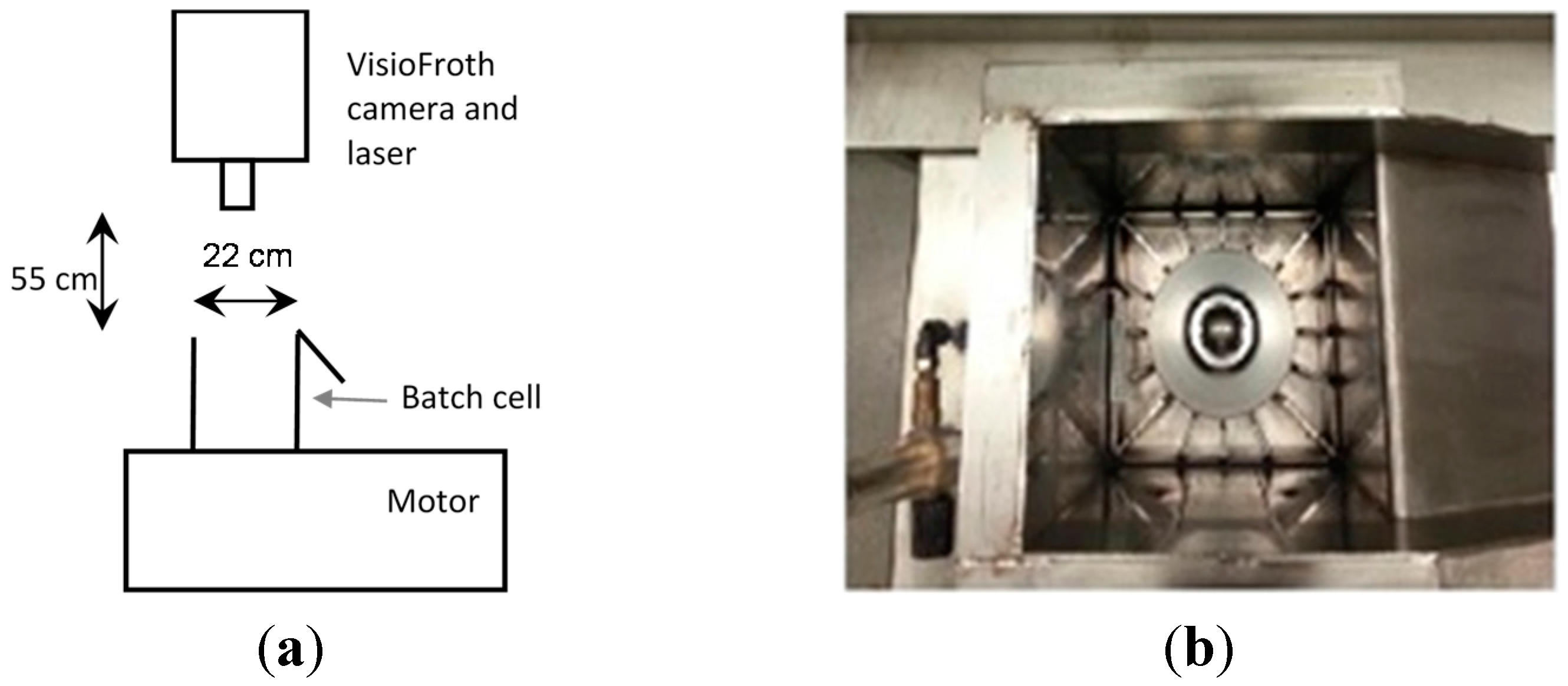
The batch flotation was monitored with a VisioFroth system (Metso^® Minerals) to capture the images at the top of the froth surface as shown in Figure 1. Hardware components of the VisioFroth system include a single IP camera, a laser, and LED lights. These images are then analysed using the software component of VisioFroth the so-called optimizing control system (OCS), to measure several image features. This image processing package is used to measure the angle and magnitude of the froth velocity, bubble distributions, color, froth texture, and stability as well as the height of the froth overflowing over the lip.

Figure 1. (a) Schematic diagram for batch flotation process equipped with VisioFroth, (b) top view of the batch flotation cell.

Figure 1. (a) Schematic diagram for batch flotation process equipped with VisioFroth, (b) top view of the batch flotation cell.

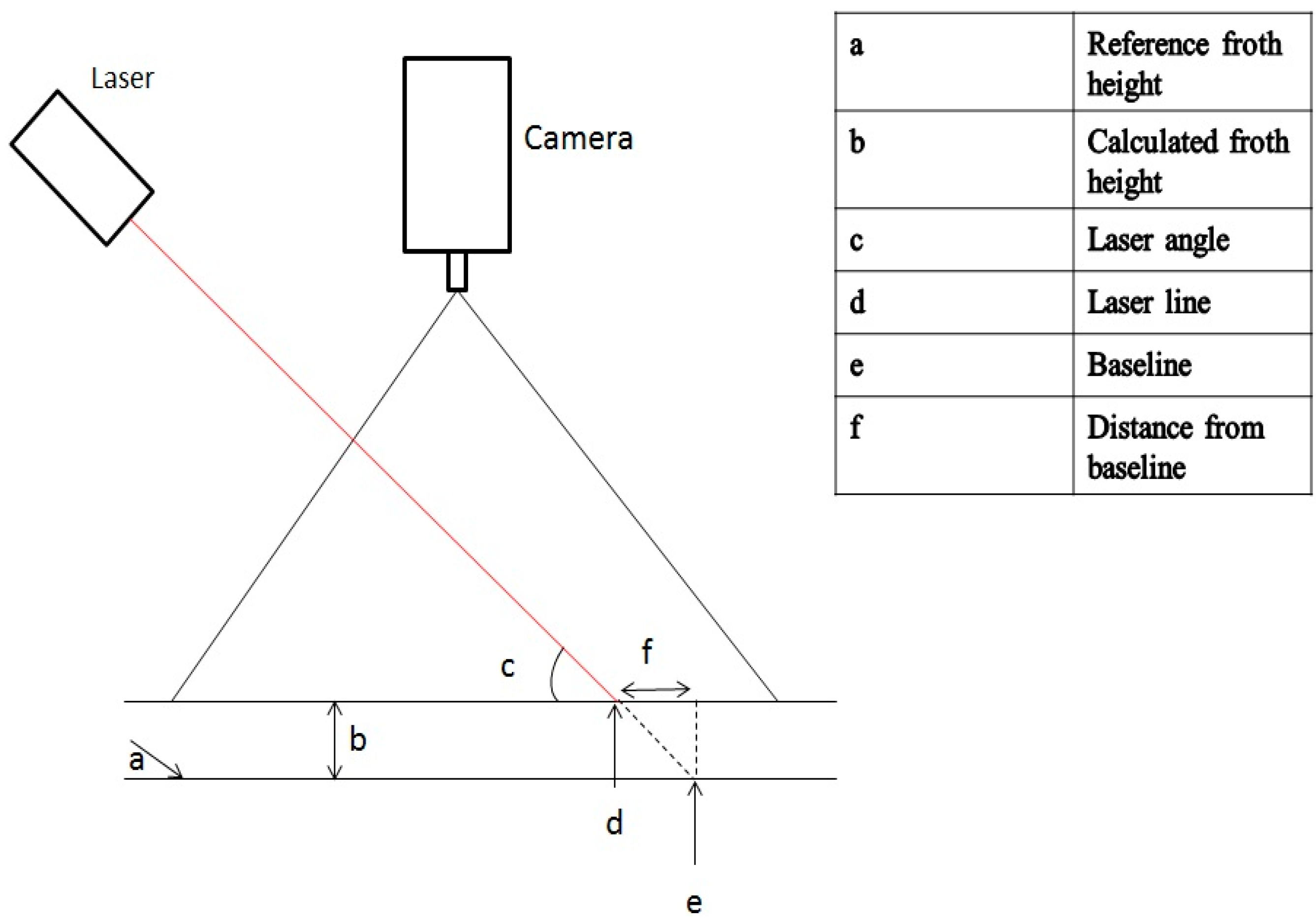
The laser is used to find the height of the overflowing froth using the change in the horizontal position of the laser line on top of the froth as shown in Figure 2. The reference froth height level corresponds to the laser being at the baseline and is at the initial time. As the froth height increases, the laser line moves a new position (d). This difference in laser line positions is used to deduce the horizontal distance from the baseline. The laser angle is set at the time of installation. The froth height (b) is calculated as:

$$b=a-f\tan (c)$$

(1)

Figure 2. Field of view and demonstration of froth height measurement using the laser light.

Figure 2. Field of view and demonstration of froth height measurement using the laser light.

Table 1 lists the various VisioFroth measurements and algorithms.

Table 1. VisioFroth measurements and algorithms.

Variable	Algorithm
Velocity	Modified Fourier transforms to calculate the displacement between two consecutive images.
Bubble size measurement	Watershed techniques are used to outline bubbles and hence calculate the bubble surface area.
Collapse rate	Calculated based on change in bubble surface area.

Table 1. VisioFroth measurements and algorithms.

Variable	Algorithm
Velocity	Modified Fourier transforms to calculate the displacement between two consecutive images.
Bubble size measurement	Watershed techniques are used to outline bubbles and hence calculate the bubble surface area.
Collapse rate	Calculated based on change in bubble surface area.

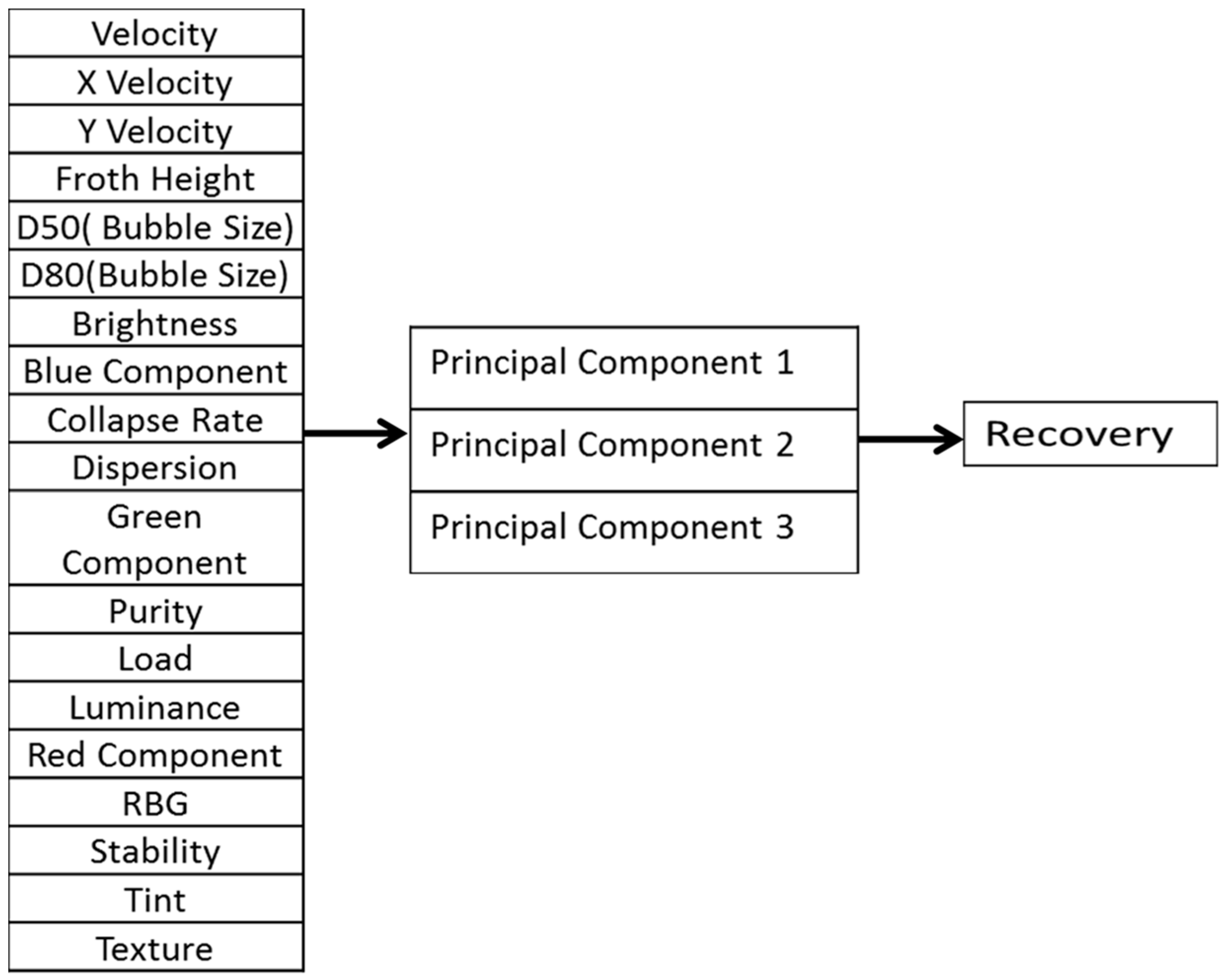
Statistical techniques, including principal component analysis (PCA) and partial least square (PLS) regression, are used to identify the important features of the images and develop a correlation for the recovery using offline measurements. The use of PCA results in dimension reduction of the data for better understanding of the given information [16]. The basic principle of this method is to represent the input matrix of data X in terms of scores (T) and loadings (P):

$$X=T{P}^T+E$$

(2)

Dimension reduction and correlation is illustrated in Figure 3 for the case of three principal components. The scores represent the projection of the original data samples onto the transformed space of reduced dimension, and the loadings represent the weights or contributions of the original variables to each principal component. Only the principal components that contribute significantly to explaining the variance in the original data are retained, and dimension reduction is obtained by truncating the number of variables based on this principle. In Equation (1), E represents the error in the representation after truncation. Thus, variables that have high loadings on the most significant principal components contribute significantly to explaining the variance in the data, and can be considered to be significant. To obtain a correlation between the input and output data, principal component regression (PCR) is employed. In PCR, regression of the score matrix from PCA is performed against the output measurement (recovery). PLSR (partial least squares regression) is also used to develop the correlation between images and recovery [17].

Figure 3. Illustration of dimension reduction using principal component analysis (PCA) with three principal components.

Figure 3. Illustration of dimension reduction using principal component analysis (PCA) with three principal components.

Potassium ethyl xanthate (KEX) and methyl isobutyl carbinol (MIBC) were used as collector and frother, respectively. Galena was obtained from Boreal Science Company in Canada in cleaved form. The galena was crushed and dry ground to −106 μm. The particle size distribution of the ground galena sample is presented in Table 2.

Table 2. Particle size distribution for galena feed.

Passing Size (μm)	Cumulative Weight %
106	100
75	96
45	37
38	30

Table 2. Particle size distribution for galena feed.

Passing Size (μm)	Cumulative Weight %
106	100
75	96
45	37
38	30

The output of the flotation process, recovery, is dependent on the air flow rate, impeller speed, collector dosage, and frother dosage. In order to capture a wide range of these operating conditions, a fractional factorial design was used to generate different operating conditions and levels of these factors, as summarized in Table 3. In each run, after selecting a desired operating condition, galena was mixed with water in the concentration of 50 g galena/1.5 L water. First, the slurry was conditioned with collector and frother for 2 and 6 min, respectively. Then, air was supplied to the cell and froth was collected at intervals of 10 s up to 100 s, and at 50 s intervals for the next 200 s. The collected froth was dried after vacuum filtration and weighed for recovery calculation. Also, images of top surface of the froth were extracted at sample time intervals of 1 s.

Table 3. Operating conditions used in the factorial experimental design.

Runs	Air Flow Rate	Impeller Peed	Frother (MIBC) Dosage	Collecter (KEX) Dosage
	(L/min)	(rpm)	(mL/L slurry)	(mol/L slurry)
1	8	500	0.042	10−5
2	14	500	0.042	10−5
3	8	1100	0.042	10−3
4	14	1100	0.042	10−5
5	8	500	0.042	10−5
6	14	500	0.1	10−5
7	8	1100	0.1	10−5
8	14	1100	0.1	10−3

Table 3. Operating conditions used in the factorial experimental design.

Runs	Air Flow Rate	Impeller Peed	Frother (MIBC) Dosage	Collecter (KEX) Dosage
	(L/min)	(rpm)	(mL/L slurry)	(mol/L slurry)
1	8	500	0.042	10−5
2	14	500	0.042	10−5
3	8	1100	0.042	10−3
4	14	1100	0.042	10−5
5	8	500	0.042	10−5
6	14	500	0.1	10−5
7	8	1100	0.1	10−5
8	14	1100	0.1	10−3

For testing the fault detection algorithm, an operating condition was selected and a step disturbance was introduced either in the air flow rate or the impeller speed. For the first disturbance test, the conditions of run 8 (described in Table 3) were used initially, and the air flow was then decreased from 14 to 8 L/min at time t = 5 s. For the second disturbance test, the conditions of run 1 were used initially, and the impeller speed was changed from 500 to 1100 rpm at time t = 5 s.

3. Model Development

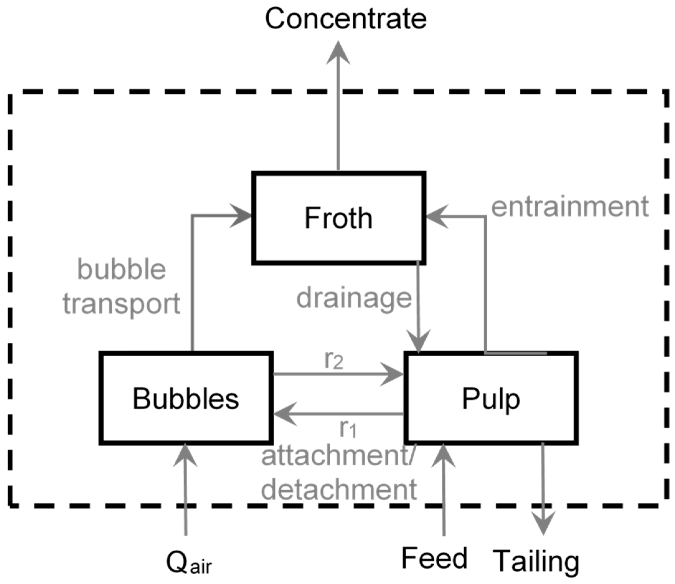
A flotation cell consists of two distinct phases: a pulp phase and a froth phase with various inter and intra-phase processes involved in the transport of material. The proposed framework in this research is based on a multi-scale approach, where attachment processes are coupled to equipment scale and inter-phase processes. This was achieved by formulating population balance, hydraulic force balance, mass transfer and kinetic rate equations for attachment and detachment and entrainment/drainage of mineral particles.

A mineral particle can be present at any of these three states, i.e., (1) attached to the bubbles in the pulp phase, (2) free in the pulp phase, or (3) attached to the bubbles in the froth phase. Particles could also be “free” in the froth phase, in water films and plateau borders, although the number of such particles may be small. However, in order to focus on the attachment and detachment, these particles were ignored in this study. The modeling framework that has been proposed is represented in Figure 4.

There are several mass transfer and kinetic processes between the three phases in the cell; they are summarized below:

• Selective attachment of mineral particles to the bubbles in the pulp phase (first order rate process, $r_1$);
• Detachment of particles from bubbles in the pulp phase (first order rate process, $r_2$);
• Transfer of particles that are attached to bubbles into the froth phase;
• Transfer of free particles from the pulp phase to the froth phase by entrainment and transfer of liquid (water) from the froth back to the pulp phase;
• Drop-back of particles from the froth to the slurry. These particles could be free particles in the froth phase, or attached particles that were detached at some point in the froth phase. At our level of modeling, we have opted for simplicity and do not distinguish between these two types of particles.

Figure 4. Schematic representation of the flotation modeling framework.

Figure 4. Schematic representation of the flotation modeling framework.

These sub-processes and recovery can be mathematically described using the following equations. The ordinary differential Equations (3)–(5) represent the mass balances for valuable mineral particles attached to the bubbles in the pulp phase, the particles that are free in the pulp phase and the particles that are attached to the bubbles in the froth phase, respectively, and Equation (6) represents the recovery of the valuable mineral particles.

$$\frac{d}{dt}\left(\mathrm{\epsilon }{V}_P{x}_b\right)=k_1\left(1-\mathrm{\epsilon }\right)V_P{x}_P-k_2\hspace{0.17em}\mathrm{\epsilon }\hspace{0.17em}{V}_P\hspace{0.17em}{x}_b-Q_{air}{x}_b$$

(3)

$$\frac{d}{dt}\left(\left(1-\mathrm{\epsilon }\right)V_P{x}_P\right)=k_2\hspace{0.17em}\mathrm{\epsilon }\hspace{0.17em}{V}_{P\hspace{0.17em}}{x}_b-k_1\left(1-\mathrm{\epsilon }\right)V_P{x}_P-Q_E{x}_P+Q_{E^{\prime }}\hspace{0.17em}{x}_c$$

(4)

$$\frac{d}{dt}\left(\mathrm{\epsilon }\hspace{0.17em}{V}_f\hspace{0.17em}{x}_c\right)=\hspace{0.17em}-\hspace{0.17em}{k}_3{V}_f{x}_c-Q_{E^{\prime }}\hspace{0.17em}{x}_c+Q_{air}{x}_b+Q_E{x}_P$$

(5)

$$y=\frac{\mathrm{\epsilon }\hspace{0.17em}{V}_f\hspace{0.17em}{t}_{samp}\hspace{0.17em}{k}_3\hspace{0.17em}{x}_c}{m_{init}}$$

(6)

Here, y is the instantaneous recovery of galena, $x_b$ is the concentration of particles on the surface of the bubbles in the pulp, $x_p$ is the concentration of particles free in the pulp, $x_c$ is the concentration of particles attached in the froth, $k_1$ is the first order rate constant for attachment,$k_2$ is the first order rate constant for detachment, $k_3$ is the rate of removal of material in the concentrate product, $\mathrm{\epsilon }$ is the volume fraction of air, $V_p$ is the volume of the pulp phase, $V_f$ is the volume of the froth phase, $Q_{air}$ is the air flow rate, $Q_E$ is the volumetric flow rate of slurry from the pulp to the froth layer, $Q_{E\prime }$ is the volumetric flow rate of liquid drainage from the froth layer to the pulp phase.

The attachment rate constant, $k_1$, and the detachment rate constant, $k_2$, are further dependent on various probabilities as discussed in the subsequent sections.

3.1. Attachment Phenomena in the Pulp Phase

Various studies have shown that the flotation process can be conceptualized as a chemical reaction [18,19]. The most general expression was proposed by Ahmed and Jameson [20]:

$$\frac{d\hspace{0.17em}{n}_P^f(t)}{dt}=\text{}\hspace{0.17em}-k^{\prime }\hspace{0.17em}{\left(n_B^f\left(t\right)\right)}^m\hspace{0.17em}{\left(n_P^f\left(t\right)\right)}^n$$

(7)

where $n_B^f\left(t\right)$ and $n_P^f\left(t\right)$are the concentrations of free bubbles and particles, $t$ is the flotation time, $k\prime$ is the pseudo-rate constant and $m$ and $n$ are the orders of the reaction with respect to bubbles and particles, respectively. The pseudo-rate constant can be expressed in terms of micro-process probabilities [21,22,23,24,25,26,27] based on the following assumptions: (1) the reaction is first order [28,29,30], (2) the bubble concentration is constant, and (3) the volume of the removed particles is negligible [20]. Therefore, Equation (7) can be written as:

$$\frac{d\hspace{0.17em}{n}_P^f\left(t\right)}{dt}=\hspace{0.17em}-k\hspace{0.17em}{n}_P^f\left(t\right)$$

(8)

where $k$ is the rate constant and can be defined as:

$$k=Z\hspace{0.17em}{P}_c\hspace{0.17em}{P}_{asl}\hspace{0.17em}{P}_{tpc}\hspace{0.17em}{P}_{stab}\hspace{0.17em}{n}_B^f\left(t\right)$$

(9)

where $Z$ is the bubble-particle collision frequency, $P_c$ is the probability of bubble-particle collision, $P_{asl}$ is the probability of bubble-particle attachment by sliding, $P_{tpc}$ is the probability of forming a three-phase contact, $P_{stab}$ is the probability of bubble-particle aggregate remaining stable during the transfer from the pulp phase to the froth phase and $n_B^f\left(t\right)$ is the concentration of bubbles without any particles attached to their surface [18].

The number of bubble-particle collisions is defined [31] as:

$$Z=5.0\hspace{0.17em}{N}_P\hspace{0.17em}{N}_B\hspace{0.17em}{d}_B^2\hspace{0.17em}{U}_t$$

(10)

where $Z$ is the number of collisions per unit time per cell volume, $N_p$ is the number of particles ready for collision, $N_B$ is the number of bubbles ready for collision, $d_B$ is the mean size of the aggregates and $U_t$ is the turbulent aggregate velocity.

Heindel and Bloom [23] proposed the probability of bubble-particle collision to be

$$P_c=\frac{1}{1+\left|G\right|}\{\frac{1}{2{\left[\frac{R_P}{R_B}+1\right]}^3}\left[2{\left(\frac{R_P}{R_B}\right)}^3+3{\left(\frac{R_P}{R_B}\right)}^2\right]+\frac{2{\mathrm{Re}}_B^{*}}{{\left[\frac{R_P}{R_B}+1\right]}^4}\left[{\left(\frac{R_P}{R_B}\right)}^3+2{\left(\frac{R_P}{R_B}\right)}^2\right]\}+\frac{\left|G\right|}{1+\left|G\right|}$$

(11)

where $R_p$ and $R_B$ are the particle and bubble radius, respectively, and $G$ is the dimensionless particle settling velocity and is defined as

$$G=\frac{v_{PS}}{v_B}$$

(12)

where $v_{ps}$ is the particle settling velocity and $v_B$ the bubble rise velocity [18].

The probability of attachment by sliding is expressed [23] as:

$$P_{asl}=\exp \{-2\left(\frac{\overline{\mathrm{\lambda }}}{C_b}\right)\left(\frac{R_P}{R_P+R_B}\right)\left(\frac{g\left(r\right)-G}{\left|k\left(r\right)\right|-G}\right)\left(\frac{h_0}{h_{crti}}-1\right)\}$$

(13)

where

$$g\left(r\right)=\left(1-\frac{3R_B}{4r}-\frac{R_B^3}{4r^3}\right)+{\mathrm{Re}}_B^{*}\left(\frac{R_B}{r}+\frac{R_B^3}{r^3}-\frac{2R_B^4}{r^4}\right)$$

(14)

$$k\left(r\right)=\hspace{0.17em}-\{\left(1-\frac{3R_B}{2r}+\frac{R_B^3}{2r^3}\right)+2{\mathrm{Re}}_B^{*}\left(\frac{R_B^4}{r^4}-\frac{R_B^3}{r^3}-\frac{R_B^2}{r^2}+\frac{R_B}{r}\right)\}$$

(15)

$$\overline{\mathrm{\lambda }}=\frac{6\text{π}\hspace{0.17em}{\mu }_l\hspace{0.17em}{R}_P}{f}$$

(16)

where r is approximately equal to $R_B+R_P$, $f$ is the fluid friction factor, $C_B$ is a constant representing the bubble surface mobility, $h_0$ is the initial thickness of the film at the time the sliding process begins and the particle starts to contact the bubble, and $h_{crit}$ is the liquid film thickness at the time that the film starts to rupture [18].

The probability of forming a three-phase contact, $P_{tpc}$, is assumed to be equal to unity, as it is considered to be a highly probable event [22].

The probability of bubble-particle aggregate stability, $P_{stab}$, is defined [25] as

$$P_{stab}=1-\exp \left(1-\frac{1}{B{o}^{\prime }}\right)$$

(17)

where

$$B{o}^{\prime }=\frac{4R_P^2\left(\mathrm{\Delta }\text{ρ}g+\frac{1.9{\text{ρ}}_P\hspace{0.17em}{\mathrm{\epsilon }}^{2/3}}{{\left(R_P+R_B\right)}^{1/3}}\right)+3R_B\left(\frac{2\text{σ}}{R_B}-2R_B\hspace{0.17em}{\text{ρ}}_l\hspace{0.17em}g\right){\sin }^2\left(\text{π}-\frac{\text{θ}}{2}\right)}{\left|6\text{σ}\sin \left(\text{π}-\frac{\text{θ}}{2}\right)\sin \left(\text{π}+\frac{\text{θ}}{2}\right)\right|}$$

(18)

where $\mathrm{\epsilon }$ is the Kolmogorov turbulent energy density, $g$ is the acceleration due to gravity, $\text{θ}$ is the contact angle, ${\text{ρ}}_p$ is the particle density and $\mathrm{\Delta }{\text{ρ}}_p=\left({\text{ρ}}_p-{\text{ρ}}_l\right)$ [18].

3.2. Detachment Phenomena in the Pulp Phase

Bloom and Heindel [18,21] developed a population balance model to include both attachment and detachment phenomena that can be considered as the equivalents of forward and reverse reactions.

$$\frac{d\hspace{0.17em}{n}_P^f\left(t\right)}{dt}=\hspace{0.17em}-k_1\hspace{0.17em}{n}_P^f\left(t\right)+k_2\hspace{0.17em}{n}_B^a\left(t\right)$$

(19)

where $n_B^a\left(t\right)$ is the concentration of the bubbles to which particles are attached on their surface, $k_1$ is the attachment rate constant and $k_2$ is the detachment rate constant. The first term in Equation (19) represents attachment phenomena by the formation of bubble-particle aggregates and the second term represents detachment phenomena in which the aggregates become unstable and do not reach the froth layer. The detachment rate constant, $k_2$, is expressed as

$$k_2=Z^{\prime }\hspace{0.17em}{P}_{destab}=Z^{\prime }\hspace{0.17em}\left(1-P_{stab}\right)$$

(20)

where $Z^{\prime }$ is the detachment frequency and $P_{destab}$ is the probability of the bubble-particle aggregate becoming unstable in the pulp phase. The detachment frequency can be expressed as

$$Z^{\prime }=\frac{\sqrt{C_{1\hspace{0.17em}}{\mathrm{\epsilon }}^{1/3}}}{{\left(d_P+d_B\right)}^{2/3}}$$

(21)

where $C_1$ is an empirical constant taken to be 2.

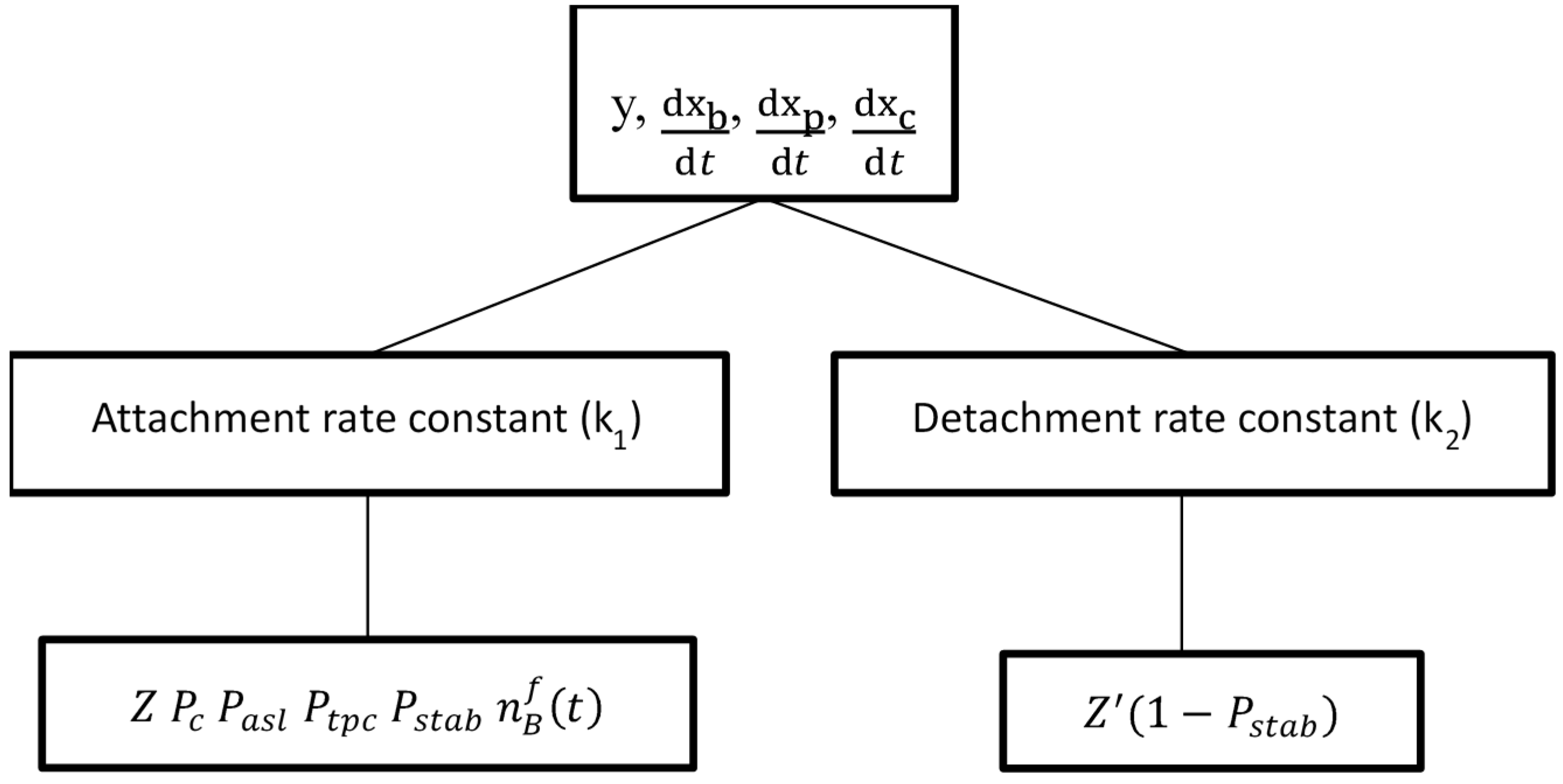
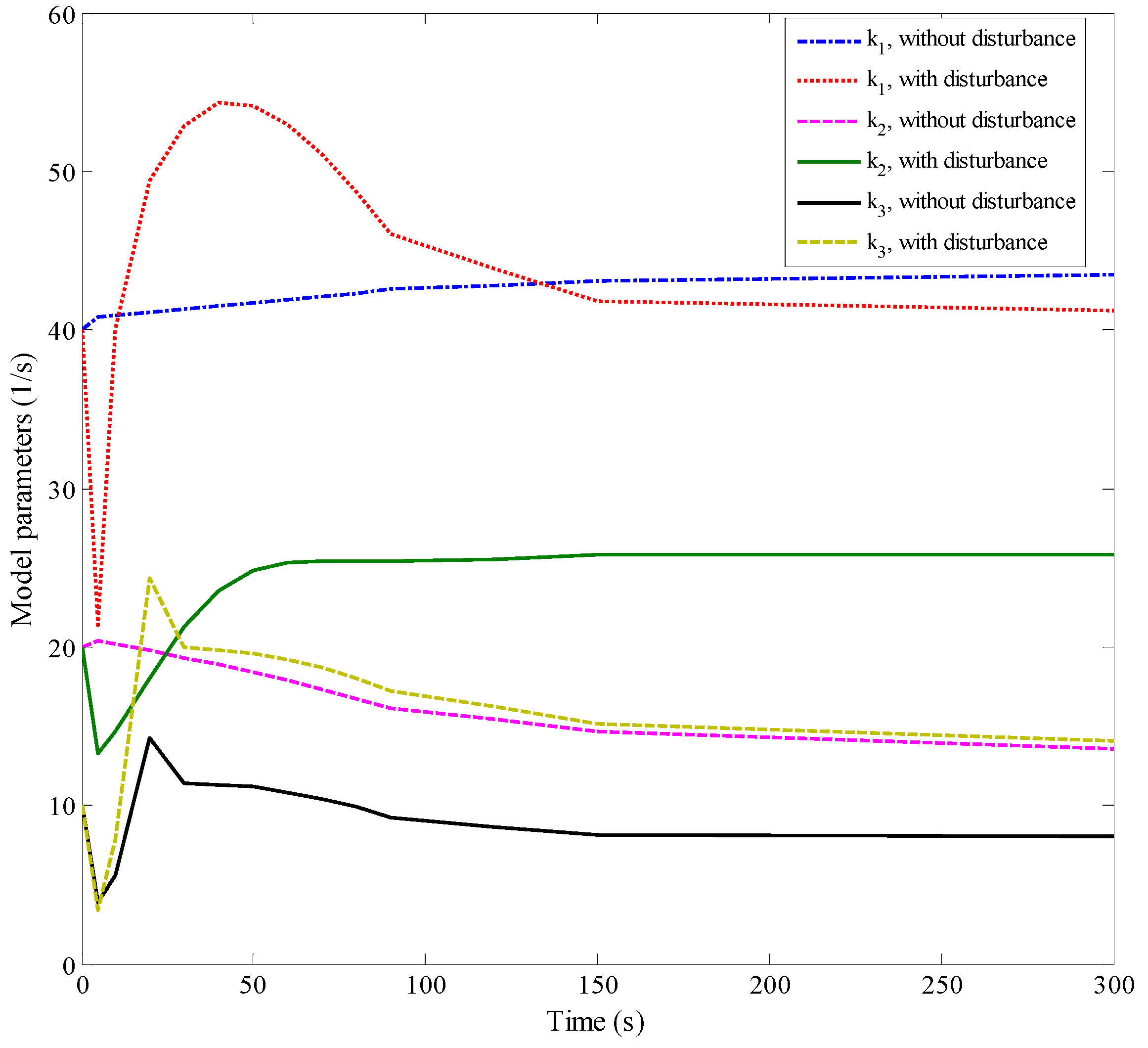
The dependence of the attachment and detachment rate constants on the probabilities of bubble-particle collision, attachment by sliding, forming a three-phase contact and aggregate stability during transfer from the pulp to the froth are summarized in Figure 5. These relations are used in the interpretation of the online estimates of parameters and disturbances affecting the system.

Figure 5. States and outputs of models and their dependence on model parameters. $y$ represents the output (recovery), $x_b$ is the concentration of particles on the surface of the bubbles in the pulp, $x_p$ is the concentration of particles free in the pulp, $x_c$ is the concentration of particles attached in the froth, $Z$ is the number of collisions per unit time per cell volume, $P_c$ is the probability of bubble-particle collision, $P_{asl}$ is the probability of attachment by sliding, $P_{tpc}$ is the probability of forming a three-phase contact, $P_{stab}$ is the probability of bubble-particle aggregate stability during transfer from the pulp to the froth phase, $n_B^f$ is the concentration and $Z\prime$ is the detachment frequency of particles.

Figure 5. States and outputs of models and their dependence on model parameters. $y$ represents the output (recovery), $x_b$ is the concentration of particles on the surface of the bubbles in the pulp, $x_p$ is the concentration of particles free in the pulp, $x_c$ is the concentration of particles attached in the froth, $Z$ is the number of collisions per unit time per cell volume, $P_c$ is the probability of bubble-particle collision, $P_{asl}$ is the probability of attachment by sliding, $P_{tpc}$ is the probability of forming a three-phase contact, $P_{stab}$ is the probability of bubble-particle aggregate stability during transfer from the pulp to the froth phase, $n_B^f$ is the concentration and $Z\prime$ is the detachment frequency of particles.

3.3. State Space Model

For parameter estimation and online updating of the proposed model, the three differential equations (Equations (3)–(5)) are expressed in state-space form. The states and the output are given by

$$\frac{dx}{dt}=Ax(t)+Bu(t)$$

(22)

$$\left[\begin{array}{l}{\dot{x}}_1\\ {\dot{x}}_2\\ {\dot{x}}_3\end{array}\right]=\left[\begin{array}{l}-a_1\hspace{0.17em}\hspace{0.17em}\hspace{0.17em}\hspace{0.17em}{a}_2\hspace{0.17em}\hspace{0.17em}\hspace{0.17em}\hspace{0.17em}\hspace{0.17em}\hspace{0.17em}\hspace{0.17em}\hspace{0.17em}\hspace{0.17em}0\\ \hspace{0.17em}\hspace{0.17em}{a}_3\hspace{0.17em}\hspace{0.17em}-a_5\hspace{0.17em}\hspace{0.17em}\hspace{0.17em}\hspace{0.17em}\hspace{0.17em}\hspace{0.17em}\hspace{0.17em}\hspace{0.17em}{a}_5\\ \hspace{0.17em}\hspace{0.17em}{a}_7\hspace{0.17em}\hspace{0.17em}\hspace{0.17em}\hspace{0.17em}\hspace{0.17em}0\hspace{0.17em}\hspace{0.17em}-\left(a_8+a_9\right)\end{array}\right]\left[\begin{array}{l}{x}_1(t)\\ x_2(t)\\ x_3(t)\end{array}\right]+\left[\begin{array}{l}0\\ a_6\\ 0\end{array}\right]$$

(23)

$$y(t)=\left[0\hspace{0.17em}\hspace{0.17em}\hspace{0.17em}\hspace{0.17em}\hspace{0.17em}0\hspace{0.17em}\hspace{0.17em}\hspace{0.17em}\hspace{0.17em}\hspace{0.17em}\frac{\mathrm{\epsilon }{V}_f\hspace{0.17em}{t}_{samp}\hspace{0.17em}{k}_3}{m_{init}}\right]\left[\begin{array}{l}{x}_1(t)\\ x_2(t)\\ x_3(t)\end{array}\right]$$

(24)

where $y$ is the instantaneous recovery of galena, $m_{init}$ is the initial mass of material in the batch flotation cell, $k_3$ is the rate of removal of material in the concentrate product, $x_1$ is the first state, i.e., the mass of solids attached to the bubbles per unit volume of pulp phase, $x_2$ is the second state, i.e., the mass of solids free in the pulp phase per unit volume of the pulp phase, and $x_3$ is the third state, i.e., the mass of solids attached to the bubbles in the froth phase. The input for the state-space model is the air flow rate. The parameters of the proposed state space model are defined in Table 4.

Table 4. Parameters used in the state space model.

Parameter	Definition
$a_1$	$k_2+\frac{Q_{air}}{\mathrm{\epsilon }{V}_p}$
$a_2$	$\frac{k_{1 }\left(1-\mathrm{\epsilon }\right)}{\mathrm{\epsilon }}$
$a_3$	$\frac{k_{2 }\mathrm{\epsilon } }{\left(1-\mathrm{\epsilon }\right)}$
$a_4$	$k_1$
$a_5$	$\frac{Q_E}{\left(1-\mathrm{\epsilon }\right)V_P}$
$a_6$	$\frac{\dot{m}}{\left(1-\mathrm{\epsilon }\right)V_P}$
$a_7$	$\frac{Q_{air}}{\mathrm{\epsilon }{V}_f}$
$a_8$	$\frac{Q_E}{\mathrm{\epsilon }{V}_f}$
$a_9$	$\frac{k_3}{\mathrm{\epsilon }}$

Table 4. Parameters used in the state space model.

Parameter	Definition
$a_1$	$k_2+\frac{Q_{air}}{\mathrm{\epsilon }{V}_p}$
$a_2$	$\frac{k_{1 }\left(1-\mathrm{\epsilon }\right)}{\mathrm{\epsilon }}$
$a_3$	$\frac{k_{2 }\mathrm{\epsilon } }{\left(1-\mathrm{\epsilon }\right)}$
$a_4$	$k_1$
$a_5$	$\frac{Q_E}{\left(1-\mathrm{\epsilon }\right)V_P}$
$a_6$	$\frac{\dot{m}}{\left(1-\mathrm{\epsilon }\right)V_P}$
$a_7$	$\frac{Q_{air}}{\mathrm{\epsilon }{V}_f}$
$a_8$	$\frac{Q_E}{\mathrm{\epsilon }{V}_f}$
$a_9$	$\frac{k_3}{\mathrm{\epsilon }}$

4. State and Parameter Estimation

4.1. Offline Estimation: Model Parameters

Model parameters were estimated by minimizing the errors between the predicted recovery and the measured recovery obtained from batch experiments for different operating conditions. Offline parameter estimation was performed by minimizing the sum of errors between the model predicted and measured recovery over the time of the batch flotation runs by using the parameter estimates ($k_1$, $k_2$, $k_3$ and ε) as decision variables. These offline estimates were used as initial guesses for online estimation.

4.2. Online Estimation: State and Parameter Estimation

The extended Kalman filter was used for online estimation of states and parameters. The EKF works in a predictor-corrector format and on the principle of optimality by minimization of the estimated error covariance. Its linear variant, the Kalman filter, is the optimal linear estimator, while the EKF provides a suboptimal estimate for nonlinear systems [10,32,33].

For a nonlinear state space model with states x and outputs y of the form

$$\dot{x}=f\left(x\left(t\right),u\left(t\right)\right)+w\left(t\right), w\left(t\right)~N\left(0,Q\right)$$

(25)

$$y\left(k\right)=g\left(x_k, u_k\right)+v\left(k\right), v\left(k\right)~N\left(0,R\right)$$

(26)

where $x_k$ is the value of the states $x$ at time $t=t_k$, and $w$ and $v$ represent the process and measurement noise, respectively, the EKF algorithm [33] consists of the prediction step:

$${\widehat{x}}_{k|k-1}=\widehat{x}\left(t_k\right), P_{k|k-1}=P\left(t_k\right)$$

(27)

obtained by integrating the differential equations from time $t_{k-1}$ to $t_k$:

$$\dot{\widehat{x}}(t)=f(\widehat{x}(t),u(t))$$

(28)

$$P(t)=F(t)P(t)+P(t)F^T(\widehat{x}(t))+Q(t),F(t)=\frac{\partial f}{\partial x}|\widehat{x}(t),u(t)$$

(29)

and the update or correction step:

$$K_k=P_{k|k-1}{G}_k^T{(G_k{P}_{k|k-1}{G}_k^T+R_k)}^{-1},G_k=\frac{\partial g}{\partial x}|{\widehat{x}}_{k|k-1}$$

(30)

$${\widehat{x}}_{k|k}={\widehat{x}}_{k|k-1}+K_k(y_k-g({\widehat{x}}_{k|k-1}))$$

(31)

$$P_{k|k}=(I-K_k{G}_k)P_{k|k-1}$$

(32)

The EKF estimate at the end of each time step is given by ${\widehat{x}}_{k|k}$, and $P_{k|k}$ represents the covariance of the state estimates. K_k is the Kalman gain at each time step t_k. Details on the augmentation of the parameters to be estimated to the state vector has been explained by Prasad et al. [10].

Parameters can be estimated by treating them as augmented states with no dynamics and forming new augmented state matrices [10]. However, observability considerations limit the maximum number of parameters to be estimated in this manner to be equal to the number of outputs; therefore, only one parameter was estimated online. However, by running multiple EKFs in parallel, each independently estimating a different parameter, the performance of the state and output estimation based on the updating of each parameter was compared. Heuristics were developed for fault detection by observing the changes in the estimates of these parameters and states in real time during the process operation, and this is described in the next section.

5. Results and Discussion

5.1. Correlation of Image Features to Recovery

Several image features were extracted using VisioFroth and correlated to the recovery measured offline using PCR and PLSR. Figure 6 shows a representative result for the experiments performed using the operating conditions for run 5 shown in Table 3. The images inset in the figure demonstrate that the image features vary with varying recovery. PCA indicates that three principal components were sufficient to capture 90% of the variance. This indicates the various extracted image features are well-correlated to each other. Features such as the velocity in the x-direction (flowing out of the cell) and the mean bubble diameter have high loadings with respect to principal component 1, and can be considered to be important variables.

Figure 6. Percentage variance (bars) and cumulative percentage variance (solid line) of the image features captured by the principal components.

Figure 6. Percentage variance (bars) and cumulative percentage variance (solid line) of the image features captured by the principal components.

PCR and PLSR were performed using five components in the input space to obtain better correlation between the image features and the recovery. A comparison of the correlated recovery against the experimental values is presented in Figure 7.

Both PLSR and PCR provide good agreement with the measured recovery values at different times; thus, either technique can be used along with image analysis to replace the assay measurement and be used online in real time. It can be concluded that froth features can provide a good description of process conditions in the form of predicting recovery. Additionally, the advantages of this technique over other methods such as online XRF include the ability to sample at shorter intervals, ease of calibration and being relatively inexpensive.

Figure 7. Comparison of principal component regression (PCR, solid line) and partial least squares regression (PLSR, dashed line) with experimental values of recovery (marker).

Figure 7. Comparison of principal component regression (PCR, solid line) and partial least squares regression (PLSR, dashed line) with experimental values of recovery (marker).

5.2. Offline Parameter Estimation

This section describes the offline fitting of the proposed model to the experimental data obtained from the batch flotation tests. In each run, the operational conditions of the experiments are input into the model and the states and the recovery were calculated and then the results are compared with the experimental data. The parameter estimates were based on obtaining the lowest error between the model predictions and experimental values for the recovery. The results for run 1 (operating conditions given in Table 3) are shown in Figure 8 with estimated values for $k_1$, $k_2$ and $k_3$ as 40, 20 and 40 s⁻¹, respectively. These parameter estimates are taken as the initial values for the online estimation using the EKF. Similar fits were obtained for the other operating conditions. The coefficient of determination ($R^2$) was greater than 86% for all the tests [34]. This indicates that the fundamental model is able to capture the dynamics of the batch process, and can be used for process monitoring and control.

Figure 8. Comparison of model predictions of cumulative recovery based on offline parameter estimation with experimental data for the batch flotation of galena.

Figure 8. Comparison of model predictions of cumulative recovery based on offline parameter estimation with experimental data for the batch flotation of galena.

5.3. Online Estimation: State and Parameter Estimation

Online estimation using the EKF is also demonstrated for the operating conditions of run 1. Three EKFs were run in parallel, and the corresponding sets of results are presented with parameter estimation for $k_1$, $k_2$, and $k_3$, respectively. Figure 9 shows the performance of the EKF-based model in predicting recovery in real-time for the case when parameter $k_1$ is being estimated. Similar results were obtained for the cases when parameters $k_2$ and $k_3$ were being estimated, respectively. Figure 10 shows the online estimates obtained for each of the parameters being updated independently. It is observed that the rate constant of attachment ($k_1$) increases and that of detachment ($k_2$) decreases with time due to the changing dynamics of the system. The rate of removal of material in the concentrate product ($k_3$) decreases with time and reaches a steady value of 13.3 s⁻¹. The final estimates are summarized in Table 5. With the model being updated in real-time, the updates in estimated values of the parameters highlight that the dependence of these dynamically varying parameters ($k_1$, $k_2$ and $k_3$) on process conditions is changing with time. This indicates that online estimation is essential for real-time monitoring, in order to be able to capture the dynamics of the changes in the parameters.

Figure 9. Comparison of real-time model predictions based on the extended Kalman filter (EKF) with experimental data for cumulative recovery when parameter k₁ is being updated.

Figure 9. Comparison of real-time model predictions based on the extended Kalman filter (EKF) with experimental data for cumulative recovery when parameter k₁ is being updated.

Table 5. Values of estimated ($k_1$, $k_2$ and $k_3$) and constant model parameters.

Parameters		Values	Remarks
Qair (L/min)	Air flow rate	8	Constant
Vp (m3)	Volume of pulp phase	1.4 × 10−3	Constant
Vf (m3)	Volume of froth phase	0.26 × 10−3	Constant
ε	Volume fraction of air	0.4	Constant
k1 (s−1)	Rate constant for attachment	Final value = 45.8	Estimated and updated (trend shown in Figure 10a)
k2 (s−1)	Rate constant for detachment	Final value = 17.1	Estimated and updated (trend shown in Figure 10b)
k3 (s−1)	Rate of removal of material in the concentrate product	Final value = 13.3	Estimated and updated (trend shown in Figure 10c)

Table 5. Values of estimated ($k_1$, $k_2$ and $k_3$) and constant model parameters.

Parameters		Values	Remarks
Qair (L/min)	Air flow rate	8	Constant
Vp (m3)	Volume of pulp phase	1.4 × 10−3	Constant
Vf (m3)	Volume of froth phase	0.26 × 10−3	Constant
ε	Volume fraction of air	0.4	Constant
k1 (s−1)	Rate constant for attachment	Final value = 45.8	Estimated and updated (trend shown in Figure 10a)
k2 (s−1)	Rate constant for detachment	Final value = 17.1	Estimated and updated (trend shown in Figure 10b)
k3 (s−1)	Rate of removal of material in the concentrate product	Final value = 13.3	Estimated and updated (trend shown in Figure 10c)

The results from online estimation are also consistent with the models for attachment and detachment described in Section 3.1 and Section 3.2. The images of the froth surface revealed that the bubble size increased with time in the batch flotation run described above. While the number of particles decreased with time as more mineral was recovered, leading to a reduction in the number of bubble-particle collisions and the probabilities of bubble-particle collision and attachment by sliding reduce slightly as the bubble size increases (Equations (9)–(11) and (13)), the probability that the bubble-particle aggregate remains stable during the transfer from the pulp phase to the froth phase increases with the increase in the bubble size. This increase in $P_{stab}$ is the dominant effect, and leads to an increase in $k_1$ (Equation (9)) and decrease in $k_2$ (Equations (17) and (18)).

Figure 10. EKF estimates of model parameters in real-time: (a) parameter k₁ being estimated, (b) parameter k₂ being estimated, and (c) parameter k₃ being estimated.

Figure 10. EKF estimates of model parameters in real-time: (a) parameter k₁ being estimated, (b) parameter k₂ being estimated, and (c) parameter k₃ being estimated.

5.4. Disturbance Identification

The ability of the EKF estimator to track changes in operation and modifying parameter estimates was also tested for two case studies with disturbances. In the first case study, a disturbance in the air flow rate was introduced at time t = 5 s in the batch cell with initial operating conditions for run 8 (shown in Table 3). At this time, the air flow rate was decreased from 14 to 8 L/min. There is a significant decrease in the cumulative recovery due to a sudden decrease in the air flow rate; this is shown in Figure 11. This is expected as lowering the air flow rate leads to lowering of the flow rate of the valuable mineral (galena) in the concentrate and hence to lower recovery. Despite the presence of the disturbance in the system, the EKF was able to track the changes by updating the states and parameters as new measurements arrive and capture the dynamics of the system satisfactorily, as seen in Figure 11.

Figure 11. Comparison of cumulative recovery profiles for run 8 (conditions defined in Table 3) with a step disturbance applied in the air flow rate (from 14 to 8 L/min) at time t = 5 s.

Figure 11. Comparison of cumulative recovery profiles for run 8 (conditions defined in Table 3) with a step disturbance applied in the air flow rate (from 14 to 8 L/min) at time t = 5 s.

Figure 12 shows the EKF-based parameter estimates for each of the parallel estimators (estimating $k_1$, $k_2$ and $k_3$, respectively), with and without the disturbance. When the disturbance was applied to the system, parameter $k_1$, which is related to the attachment of particles, and parameter $k_2$, which is related to the detachment of particles, did not change significantly in comparison to the condition when there was no disturbance. However, parameter $k_3$, which is related to the rate of transfer of particles to the concentrate from the froth phase, decreased because lowering the air flow rate resulted in a decrease in the number of the particles that are brought from the pulp phase to the froth phase; consequently, the rate of transfer of particles to the concentrate product would be decreased as well.

Figure 12. Comparison of real-time parameter estimates (k₁, k₂ or k₃ being estimated) for run 8 with the step disturbance in the air flow rate.

Figure 12. Comparison of real-time parameter estimates (k₁, k₂ or k₃ being estimated) for run 8 with the step disturbance in the air flow rate.

Additionally, the estimated states of the system are shown in Figure 13. As is expected, the only system state that changes with a disturbance in the air flow is the concentration of the particles attached in the pulp. This slight increase is observed due to a decrease in the transfer of particles from the pulp to the froth.

Figure 13. Real-time state estimates using the EKF for run 8 with the step disturbance in the air flow rate ($x_b$: concentration of particles on the surface of the bubbles in the pulp, $x_p$: concentration of particles free in the pulp, $x_c$: concentration of particles attached in the froth).

Figure 13. Real-time state estimates using the EKF for run 8 with the step disturbance in the air flow rate ($x_b$: concentration of particles on the surface of the bubbles in the pulp, $x_p$: concentration of particles free in the pulp, $x_c$: concentration of particles attached in the froth).

The second case study was based on the initial operating conditions for run 1 (given in Table 3), with the impeller speed being increased from 500 to 1100 rpm at time t = 5 s to create a step disturbance. Increasing the impeller speed in the pulp phase increases the bubble count and the bubble-particle interactions. This leads to an increase in the probability of bubble-particle collision and therefore attachment (Equations (9) and (10)), leading to an increase in the particles brought into the froth phase and consequently in the concentrate. Figure 14 shows the EKF estimates for each of the parallel estimators for the three parameters of the system ($k_1$, $k_2$ and $k_3$), with and without the disturbance. The estimates of parameters $k_2$ and $k_3$ did not change significantly but $k_1$, the rate of attachment, decreased initially due to the increased turbulence, and then increased due to the larger number of interactions between bubbles and particles.

The changes in the estimated states for the case with the disturbance in the impeller speed are similar to those for the case with the air flow disturbance, as is shown in Figure 15. This indicates that monitoring of the parameters, and not the states, is preferred for tracking these types of disturbances in the system, since the estimates of the parameters are more sensitive to the presence, size, and type of disturbances present in the system. These results provide a proof of concept that heuristics related to online parameter estimation using parallel EKFs (negative step changes in the air flow rate being detected by a reduction in the value of the parameter estimate for $k_3$, and positive step changes in the impeller speed being detected by a decrease and then an increase in the parameter estimate for $k_1$) can be developed and used for process monitoring and fault diagnosis in froth flotation processes, and are consistent with the fundamental processes involved in attachment and detachment of particles to bubbles, their transfer from the pulp to the froth and their eventual recovery in the concentrate. Our future work aims to extend this proof of concept to more complex ores and continuous flotation processes, and to develop rigorous algorithms for process monitoring under any operating conditions and disturbances.

Figure 14. Comparison of parameter estimates ($k_1$, $k_2$ or $k_3$ being estimated) for run 1 with a step disturbance applied in the impeller speed from 500 to 1100 rpm at time t = 5s.

Figure 14. Comparison of parameter estimates ($k_1$, $k_2$ or $k_3$ being estimated) for run 1 with a step disturbance applied in the impeller speed from 500 to 1100 rpm at time t = 5s.

Figure 15. Real-time state estimates using the EKF for run 1 with the step disturbance in the impeller speed ($x_b$: concentration of particles on the surface of the bubbles in the pulp, $x_p$: concentration of particles free in the pulp, $x_c$: concentration of particles attached in the froth).

Figure 15. Real-time state estimates using the EKF for run 1 with the step disturbance in the impeller speed ($x_b$: concentration of particles on the surface of the bubbles in the pulp, $x_p$: concentration of particles free in the pulp, $x_c$: concentration of particles attached in the froth).

6. Conclusions

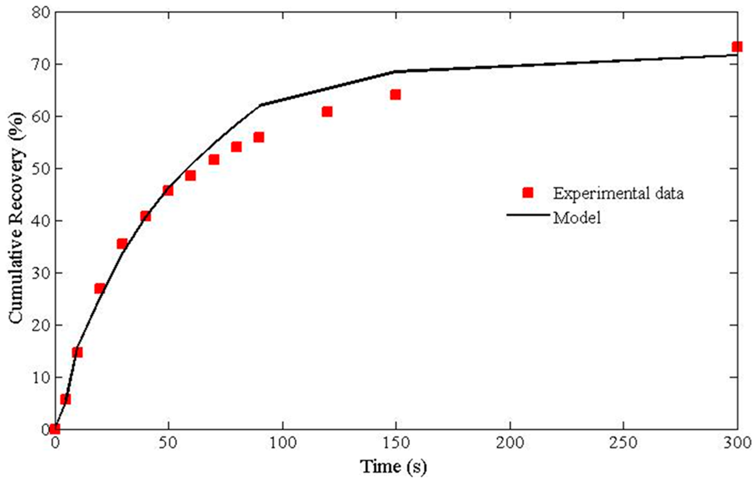
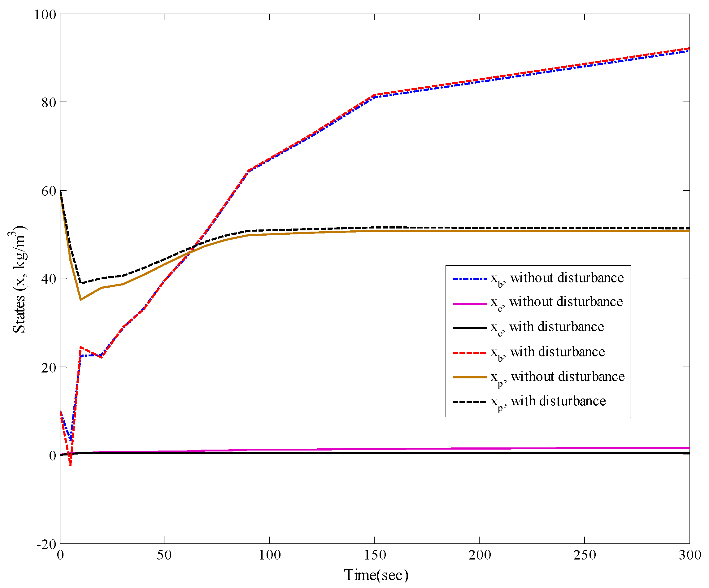
A fundamental model for batch froth flotation was developed based on descriptions of bubble-particle collision, attachment, and detachment coupled with bubble and liquid transport. Real-time measurements of froth bubble size and velocity utilizing image processing techniques were injected into the model. Offline parameter estimation was used to verify the validity of this model for describing the dynamics of batch froth flotation processes.

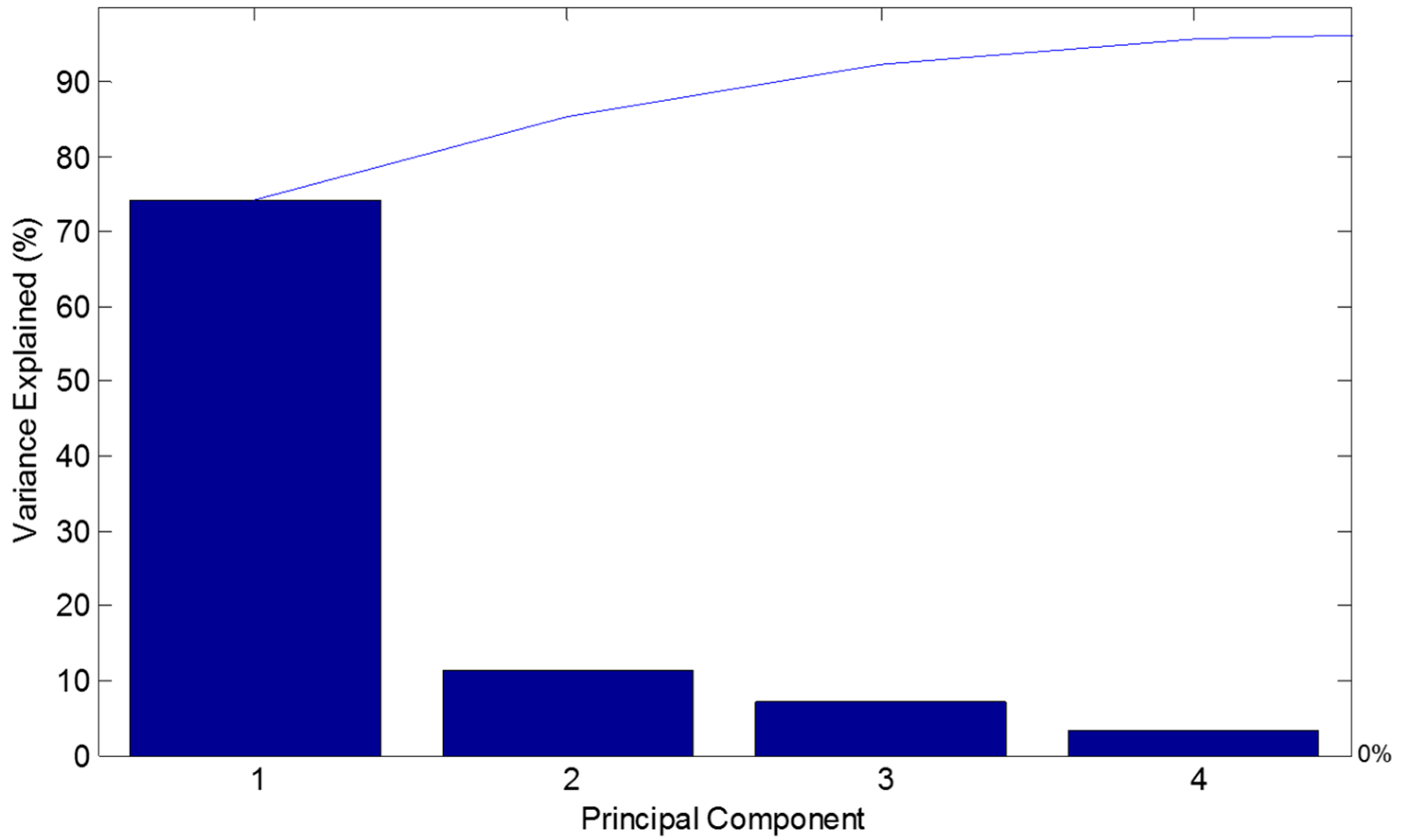
Statistical methods such as principal component regression and partial least squares regression were used to calibrate the real-time froth surface images against the recovery measured offline. Both the methods described the recovery well in real time and were successful in reducing the dimension of image features significantly without any substantial loss of information or prediction capability.

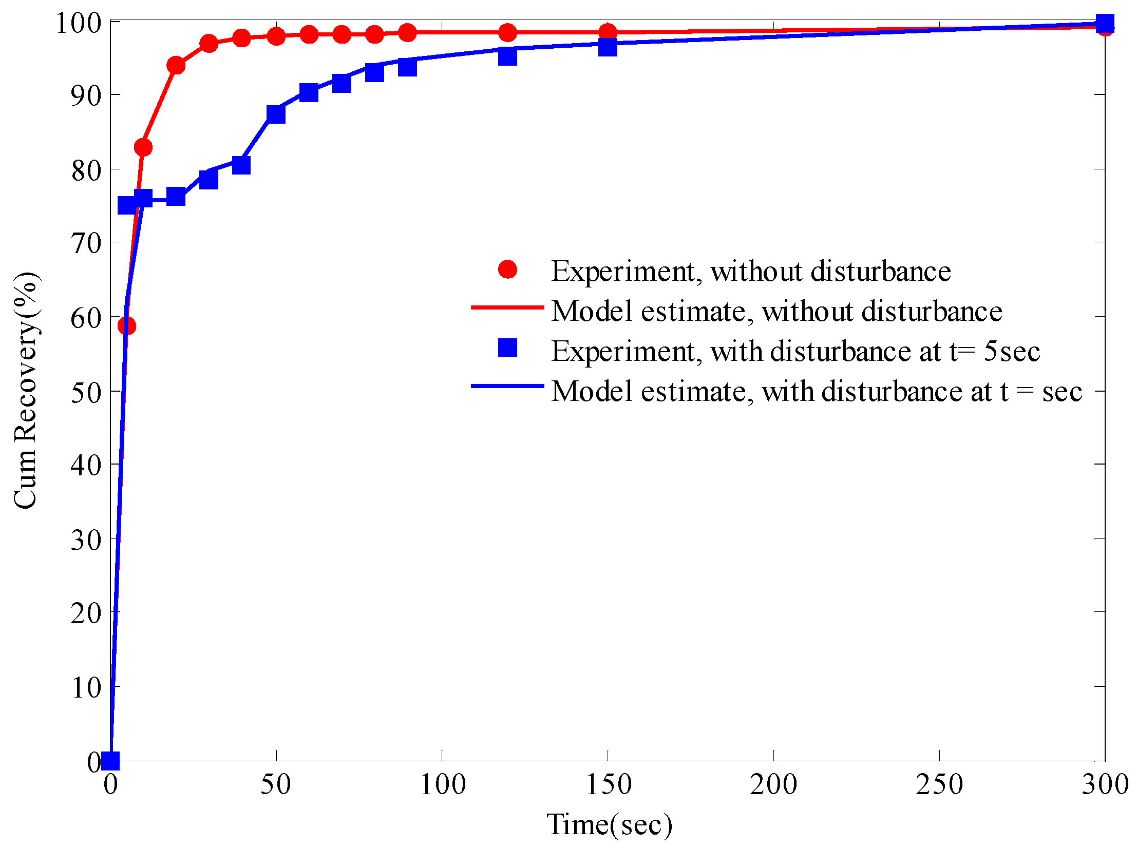
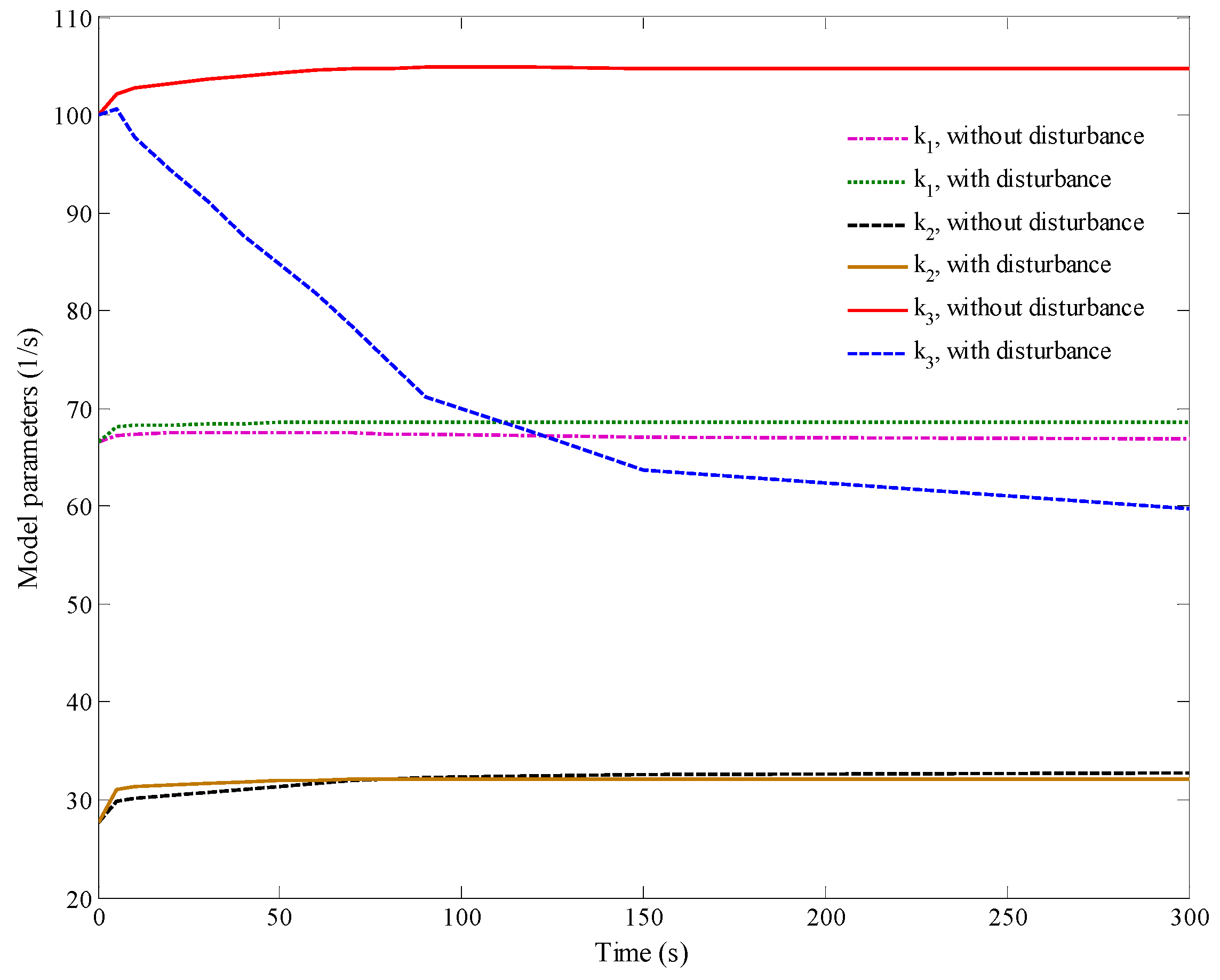
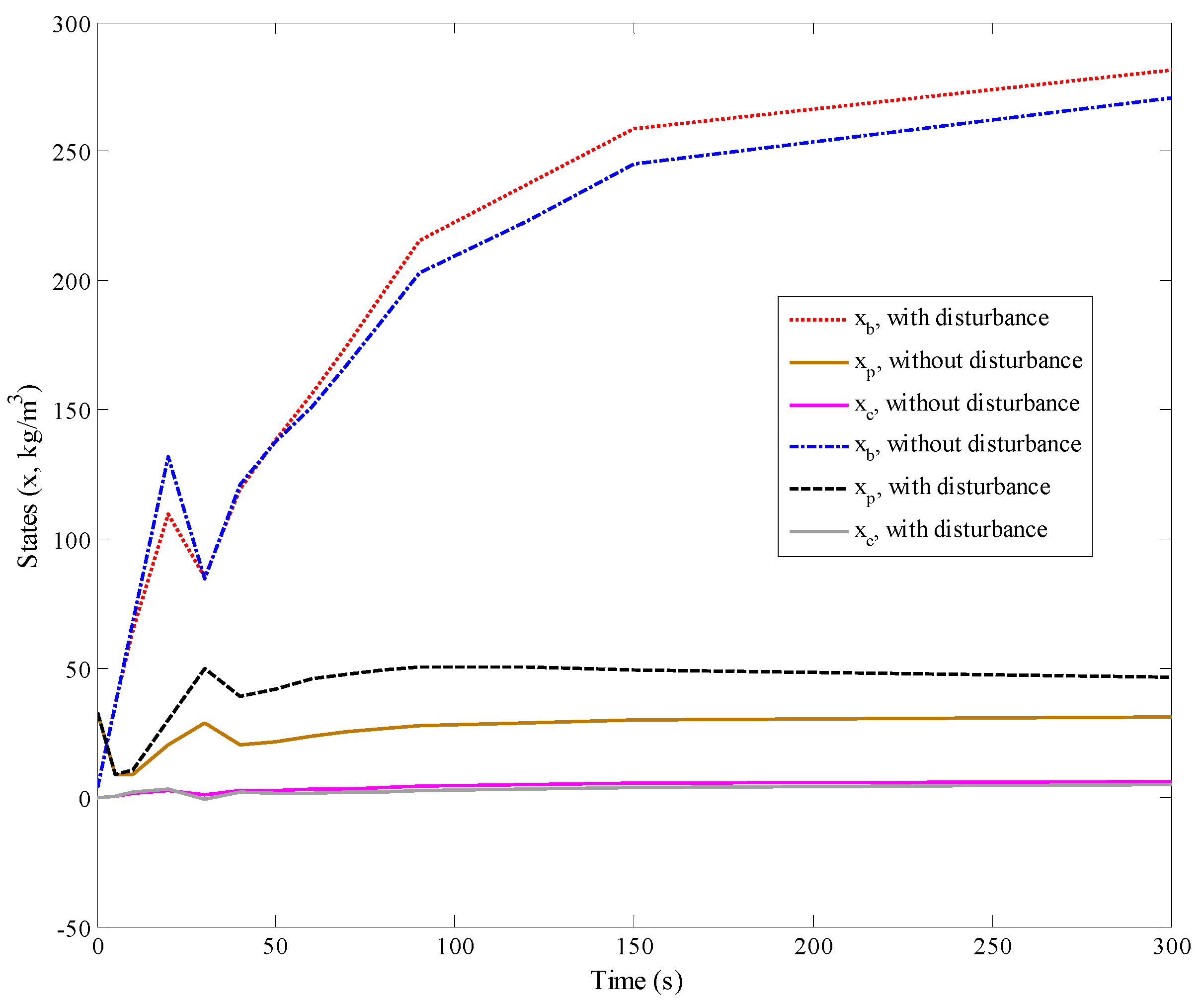
Methods based on advanced state and parameter estimation techniques (extended Kalman filtering) were used to update the models and their parameter estimates in real time based on the online measurements. Validation with experiments confirmed that process dynamics were captured both in normal operations as well as in the presence of disturbances affecting the batch flotation process.

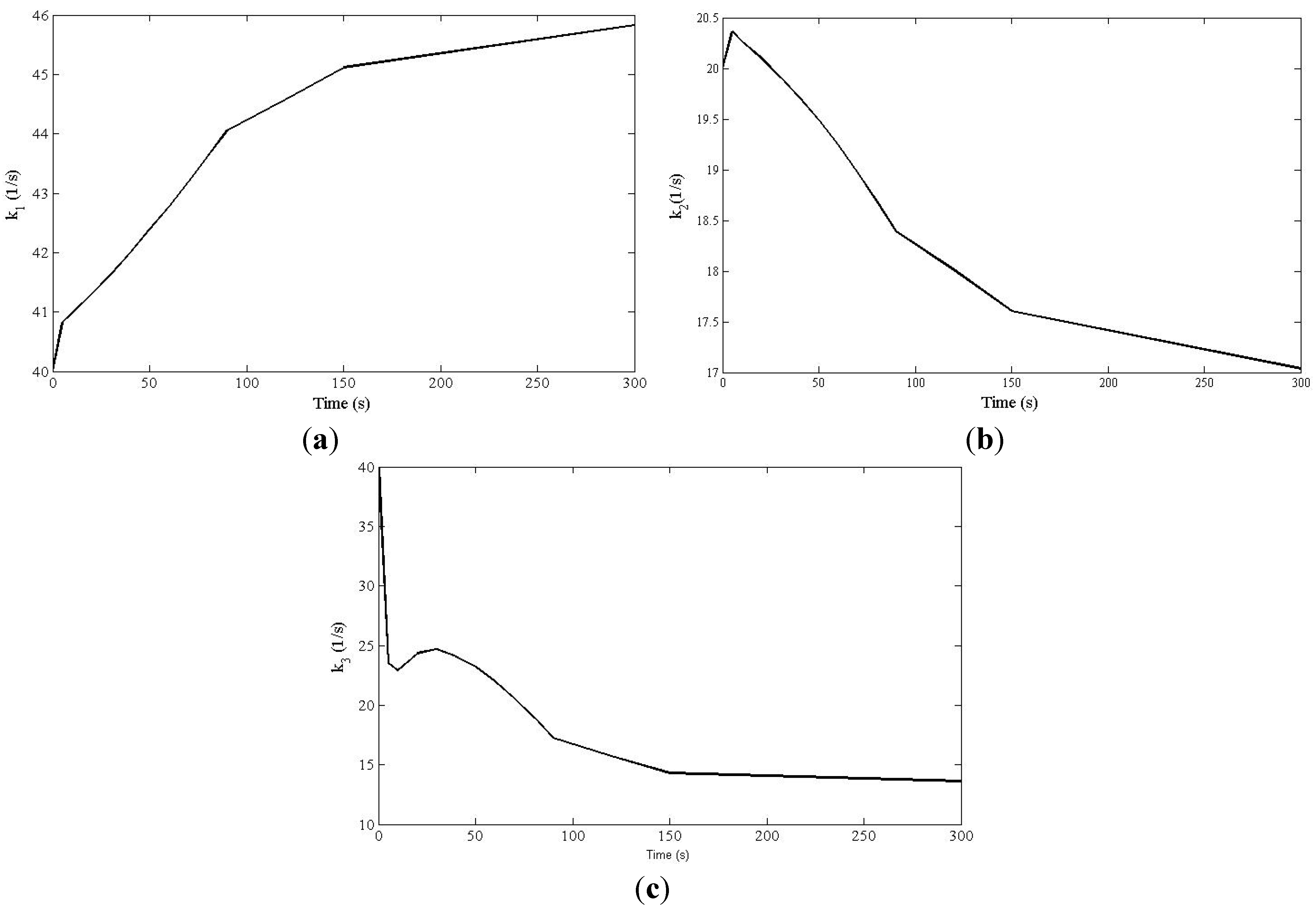
Disturbances in the air flow rate and impeller speed were induced in the system. Based on the updated parameter estimates (using the EKF), heuristics were developed and validated that could discriminate between various disturbances affecting the system, thus providing a proof of concept that monitoring using real-time updated fundamental models provides physical insight into the batch flotation process.

References

1. Fuerstenau, M.C.; Jameson, G.J.; Yoon, R.H. Froth Flotation: A Century of Innovation; Society for Mining, Metallurgy and Exploration: Littleton, CO, USA, 2007. [Google Scholar]
2. Bouchard, J.; Desbiens, A.; Villar, R.D. Recent advances in bias and froth depth control in flotation columns. Miner. Eng. 2005, 18, 709–720. [Google Scholar] [CrossRef]
3. Del Villar, R.; Grégoire, M.; Pomerleau, A. Automatic control of a laboratory flotation column. Miner. Eng. 1999, 12, 291–308. [Google Scholar] [CrossRef]
4. Maffei, A.C.; de Oliveira Luz, I.L. Pulp-froth interface control in the flotation column. Dev. Miner. Process. 2000, 13. [Google Scholar] [CrossRef]
5. Neethling, S.J.; Cilliers, J.J. Solids motion in flowing froths. Chem. Eng. Sci. 2002, 57, 607–615. [Google Scholar] [CrossRef]
6. Neethling, S.J.; Lee, H.T.; Cilliers, J.J. Simple relationships for predicting the recovery of liquid from flowing foams and froths. Miner. Eng. 2003, 16, 1123–1130. [Google Scholar] [CrossRef]
7. Neethling, S.J.; Cilliers, J.J. The entrainment factor in froth flotation: Model for particle size and other operating parameter effects. Int. J. Miner. Process. 2009, 93, 141–148. [Google Scholar] [CrossRef]
8. Geetha, M.; Kumar, P.A.; Jerome, J. Comparative assessment of a chemical reactor using extended Kalman filter and unscented Kalman filter. Procedia Technol. 2014, 14, 75–84. [Google Scholar] [CrossRef]
9. Höckerdal, E.; Frisk, E.; Eriksson, L. EKF-based adaptation of look-up tables with an air mass-flow sensor application. Control Eng. Pract. 2011, 19, 442–453. [Google Scholar] [CrossRef]
10. Prasad, V.; Schley, M.; Russo, L.P.; Bequette, B.W. Product property and production rate control of styrene polymerization. J. Process Control 2002, 12, 353–372. [Google Scholar] [CrossRef]
11. Benkouider, A.M.; Buvat, J.C.; Cosmao, J.M.; Saboni, A. Fault detection in semi-batch reactor using the EKF and statistical method. J. Loss Prev. Process Ind. 2009, 22, 153–161. [Google Scholar] [CrossRef]
12. Moolman, D.W.; Eksteen, J.J.; Aldrich, C.; van Deventer, J.S.J. The significance of flotation froth appearance for machine vision control. Int. J. Miner. Process. 1996, 48, 135–158. [Google Scholar] [CrossRef]
13. A Correlation Between VisioFroth™ Measurements and the Performance of a Flotation Cell. Available online: http://www.metso.com/miningandconstruction/mct_service.nsf/WebWID/WTB-120118-22576-F1987/$File/136.pdf (accessed on 25 August 2015).
14. Aldrich, C.; Marais, C.; Shean, B.J.; Cilliers, J.J. Online monitoring and control of froth flotation systems with machine vision: A review. Int. J. Miner. Process. 2010, 96, 1–13. [Google Scholar] [CrossRef]
15. Leiva, J.; Vinnett, L.; Yianatos, J. Estimation of air recovery by measuring froth transport over the lip in a bi-dimensional flotation cell. Miner. Eng. 2012, 36, 303–308. [Google Scholar] [CrossRef]
16. Jolliffe, I. Principal Component Analysis; Springer-Verlag: New York, NY, USA, 2002. [Google Scholar]
17. Geladi, P.; Kowalski, B.R. Partial least-squares regression: A tutorial. Anal. Chim. Acta 1986, 185, 1–17. [Google Scholar] [CrossRef]
18. Bloom, F.; Heindel, T.J. Modeling flotation separation in a semi-batch process. Chem. Eng. Sci. 2003, 58, 353–365. [Google Scholar] [CrossRef]
19. Jameson, G.J.; Nam, S.; Young, M.M. Physical factors affecting recovery rates in flotation. Miner. Sci. Eng. 1977, 9, 103–118. [Google Scholar]
20. Ahmed, N.; Jameson, G.J. Flotation kinetics. Miner. Process. Extr. Metall. Rev. 1989, 5, 77–99. [Google Scholar] [CrossRef]
21. Bloom, F.; Heindel, T.J. Mathematical modelling of the flotation deinking process. Math. Comput. Model. 1997, 25, 13–58. [Google Scholar] [CrossRef]
22. Bloom, F.; Heindel, T.J. On the structure of collision and detachment frequencies in flotation models. Chem. Eng. Sci. 2002, 57, 2467–2473. [Google Scholar] [CrossRef]
23. Heindel, T.J.; Bloom, F. Exact and approximate expressions for bubble–particle collision. J. Colloid Interface Sci. 1999, 213, 101–111. [Google Scholar] [CrossRef] [PubMed]
24. Amand, J.S.F. Hydrodynamics of deinking flotation. Int. J. Miner. Process. 1999, 56, 277–316. [Google Scholar] [CrossRef]
25. Schulze, H.J. Probability of particle attachment on gas bubbles by sliding. Adv. Colloid Interface Sci. 1992, 40, 283–305. [Google Scholar] [CrossRef]
26. Schulze, H.J. Physico-Chemical Elementary Processes in Flotation: An Analysis From the Point of View of Colloid Science Including Process Engineering Considerations; Elsevier: Amsterdam, The Netherlands, 1984. [Google Scholar]
27. Schulze, H.J. The fundamentals of flotation deinking in comparison to mineral flotation. In Proceeding of the 1st Research Forum on Recycling, Toronto, ON, Canada, 29–31 October 1991; pp. 161–167.
28. Nguyen, A.V.; Ralston, J.; Schulze, H.J. On modelling of bubble–particle attachment probability in flotation. Int. J. Miner. Process. 1998, 53, 225–249. [Google Scholar] [CrossRef]
29. Woodburn, E.T. Mathematical modelling of flotation processes. Miner. Sci. Eng. 1970, 2, 3–17. [Google Scholar]
30. Yoon, R.H.; Mao, L. Application of extended DLVO theory, IV: Derivation of flotation rate equation from first principles. J. Colloid Interface Sci. 1996, 181, 613–626. [Google Scholar] [CrossRef]
31. Bascur, O.A. An interactive dynamic flotation model framework. Dev. Miner. Process. 2000, 13. [Google Scholar] [CrossRef]
32. Kalman, R.E. A new approach to linear filtering and prediction problems. J. Fluids Eng. 1960, 82, 35–45. [Google Scholar] [CrossRef]
33. Gelb, A. Applied Optimal Estimation; MIT Press: Cambridge, MA, USA, 1974. [Google Scholar]
34. Sekhavat, M. Real-Time Updating of A Dynamic Fundamental Model for Froth Flotation Process. Master’s Thesis, University of Alberta, Edmonton, AB, Canada, 2014. [Google Scholar]