Combining Laser-Induced Breakdown Spectroscopy with the Standard Addition Method for Analyzing Impurity Elements in the Lithium Ore Mineral Spodumene

Abstract

Spodumene (LiAlSi₂O₆) is a key lithium source mineral for energy storage devices, making the accurate and rapid analysis of its elemental composition crucial for the battery industry. This study explores the use of laser-induced breakdown spectroscopy (LIBS) combined with the standard addition method to analyze Be, Na, and K in spodumene. The method achieved relative errors of 5%–15% compared to inductively coupled plasma optical emission spectroscopy (ICP-OES), without requiring certified standards. To ensure accuracy, non-resonance emissions were used for Be and Na to minimize self-absorption effects. Although K analysis faced challenges due to strong self-absorption in resonance emissions, focusing on weak edge intensity reduced the relative error significantly. Our results suggest that LIBS combined with the standard addition method is a promising approach for lithium ore analysis, eliminating the need for certified standard materials and complex sample preparation steps such as acid digestion and high-factor dilution.

1. Introduction

Lithium is crucial for energy storage devices like Li-ion batteries [1]. Consequently, the global need for Li has increased, and the European Commission included it in the list of critical raw materials in 2020 [2]. Australia, Chile, Argentina, and China are the major producers of Li [3]. Spodumene (LiAlSi₂O₆) is one of the major lithium-bearing minerals [4,5]. Spodumene comprises approximately 8.03% Li₂O from theoretical estimation based on the chemical formula [6]. It also contains various elements such as Na, Ti, V, Cr, Mn, Fe, Zn, Ga, Ge, Ta, Nb, Rb, K, Be, Cs, W, Mo, and Sn [4,7,8]. The presence of impurity elements can intensify the color of different types of spodumene gemstones [9,10,11]. Moreover, excessive quantities of these elements can lead to unfavorable alterations in processing spodumene as a lithium ore [5]. Impurity elements can also impact the stability of spodumene [4]. The intra-crystalline distribution of impurity elements in spodumene-bearing pegmatite is anticipated to provide deeper insight into its origins [4], which is crucial for assessing the purity of lithium ore [5]. Hence, it is important to identify and quantify the impurity elements in spodumene to facilitate Li-based energy storage technology.

X-ray fluorescence (XRF) and inductively coupled plasma optical emission spectroscopy (ICP-OES) are widely used for elemental analysis of ores [5,12,13]. However, XRF has limited sensitivity for light elements like Na due to their low X-ray energies, which are easily absorbed by air [14]. While ICP-OES effectively detects light elements, it requires costly operation, complex acid digestion, and dilution steps that risk contamination [15]. As a result, analyzing impurity light elements in refractory ores such as spodumene remains challenging. Laser-induced breakdown spectroscopy (LIBS) uses a focused laser pulse to generate plasma on a sample’s surface, emitting light that reveals the sample’s elemental composition [16]. LIBS can analyze solids, liquids, and gases, and detect nearly all elements, including light ones that XRF struggles to detect [13]. Unlike methods such as ICP-OES, inductively coupled plasma mass spectrometry (ICP-MS), and atomic absorption spectroscopy (AAS), LIBS requires no acid digestion or dilution, making it a faster and more versatile technique.

The response of analyte signals from LIBS differs even for the same concentration of the analyte when the samples have different matrices [17]. This matrix effect can significantly influence the accuracy of the ordinary calibration curve method which is based on the correlation between the signal intensities and the analyte concentrations [18,19,20,21,22,23,24]. Thus, the LIBS analysis using the intensity-to-concentration calibration curves strictly requires the standards of which matrix is sufficiently close to that of the sample. However, matrix-matched standards are not always instantly available, particularly for newly emerging materials, which require separate elaboration to develop the standard materials for the use of chemical analysis. There are a few reports on the application of the standard addition method combined with LIBS to overcome the matrix effect on the analytical performances [15,25,26]. The traditional standard addition method can also be considered to avoid the matrix effect in LIBS analysis [27]. The standard addition method involves preparing a set of standard materials by incorporating varying concentrations of the analytes in the samples. Thus, the standards prepared in this way have the same matrix with that of the sample. The analyte signal intensities of the unspiked and spiked samples, composing the set of standards, are then used to construct a calibration curve. The analyte concentration in the unspiked sample is estimated by extrapolating the calibration curve to the point corresponding to zero analyte signal intensity. Hence, LIBS combined with the standard addition method can be considered an alternative approach for the accurate quantification of analyte elements in the sample without the need for separately prepared matrix-matched certified standard materials [15,25,26]. In spite of this advantage, the standard addition method has been rarely employed in LIBS analysis. The success of the standard addition method mainly depends on how accurately the signal sensitivity to the analyte concentration is obtained. Compared with other conventional elemental analysis techniques such as ICP-OES, ICP-MS, and AAS, LIBS demonstrates the larger uncertainty in sensitivity. Moreover, the optical emission signals measured in LIBS can be easily influenced by self-absorption since the LIBS plasma is not spatially homogeneous. Particularly, the self-absorption effect becomes stronger for samples or standards containing analytes at the higher concentrations. This results in lower signal sensitivity than needed for extrapolation to zero analyte concentration, leading to the overestimation of the analyte concentration in the sample. To analyze impurity elements, strong emission lines are preferred, and the strong emission lines are mostly resonance lines whose lower level is the ground state. Resonance lines are most sensitive to the self-absorption. This is a dilemma between detectability and sensitivity.

In this work, we evaluated the feasibility of LIBS combined with the standard addition method for the quantitative analysis of Be, Na, and K in spodumene. While Li is undoubtedly the primary element of interest in spodumene, the quantification of impurity elements such as Na, K, and Be is also of critical importance. These elements significantly influence the processing behavior of spodumene in industrial refining, as they can affect the purity of the final lithium compounds such as LiOH or Li₂CO₃ and reduce the efficiency of the extraction process. Moreover, certain impurity elements (e.g., Be) may have economic value on their own, and their presence offers useful insights into the geochemical history and classification of lithium-bearing ores. Therefore, accurate analysis of Na, K, and Be plays a key role in resource evaluation, quality control, and process optimization for lithium extraction. This method enabled us to determine the concentrations of these elements with relative errors of 5%–15% compared to ICP-OES, without the need for certified standard materials. Achieving accurate results required suppressing the self-absorption effect on analyte signals. We used the non-resonance emissions of Be I at 332.1 nm and Na I at 819.5 nm for Be and Na analysis, as these lines are less affected by self-absorption than resonance lines. However, suitable non-resonance emissions were not available for K, and the strong resonance emissions of K I at 766.5 nm and 769.9 nm were significantly impacted by self-absorption, resulting in an overestimation of K concentrations. Alternatively, using weak edge intensities of the resonance line profile centered at 766.5 nm for the standard addition method reduced the relative error remarkably from 420% to 5.5%. Considering (i) the laser-ablation sampling process of LIBS, which eliminates the need for acid digestion and dilution required for ICP-OES, and (ii) the simultaneous multi-elemental analysis capability of LIBS, including Na and the lighter elements that XRF struggles to detect, LIBS combined with the standard addition method presents a reliable alternative to ICP-OES and XRF for spodumene analysis.

2. Materials and Methods

2.1. ICP-OES Analysis

Spodumene ores extracted from the Pilbara mine in Australia are imported into the Republic of Korea and processed to produce LiOH, which is used as a precursor for cathode materials in lithium-ion batteries. The sample used in this study was part of the spodumene ore from the Pilbara mine. For ICP-OES analysis, the spodumene sample was first homogenized using a ball mill and 0.2 g of the homogenized powder was taken and put in the Teflon bottle for acid digestion with heating. A mixture of nitric acid solution (70% aqueous solution, ODLAB, Kwangmyung, Republic of Korea) and hydrochloric acid solution (35% aqueous solution, ODLAB, Kwangmyung, Republic of Korea) was prepared with a volume ratio of 1:3. An amount of 9 mL of this acid mixture solution was added in the Teflon bottle. An amount of 1 mL of fluoric acid solution (50% aqueous solution; ODLAB, Kwangmyung, Republic of Korea) was also added in the Teflon bottle. The bottle containing the homogenized spodumene powder and the acid mixture solution was tightened and heated on the heating block (ODLAB ECOPRE-I; ODLAB, Kwangmyung, Republic of Korea), of which the temperature was set to 230 °C for 1 h. Opening the bottle, the acid was then allowed to evaporate out at 180 °C. When the volume of the remaining solution became 1–2 mL, the acid evaporation was stopped. The remaining solution was diluted by adding distilled water to obtain a 20 mL solution. Finally, the diluted solution was filtered using a polyvinylidene fluoride filter (0.45 μm, Thermo Fisher Scientific, Waltham, MA, USA). Standard solutions for ICP-OES analysis of Be, Na, and K in the concentration range between 0.1 and 10 mg/kg were prepared by diluting the multi-standard solution (Calib. Std No. 4, AccuStandard, New Haven, CT, USA). The spodumene sample solution and the standard solutions of Be, Na, and K were introduced in the ICP-OES spectrometer at the flow rate of 2 mL/min. The radio-frequency power of the ICP-OES was set to 1400 W. The coolant, auxiliary, and nebulizer argon gases were flowed at rates of 13, 1, and 0.96 L/min, respectively. Emission lines of Be, Na, and K at 313.042, 589.592, and 766.491 nm, respectively, were used for the analysis. The ICP-OES spectrometer (SPECTROGREEN; SPECTRO, Kleve, Germany), located at the Plasma Spectroscopy Analysis Center, one of the core facilities supported by the Korea Basic Science Institute (National Research Facilities and Equipment Center, Daejeon, Republic of Korea), was used in this work.

2.2. LIBS Analysis

The finely ground spodumene powder was used to prepare the standards containing different relative concentrations of the analytes for the standard addition method. High-purity (≥99%) beryllium oxide (BeO) and potassium superoxide (KO₂) powders from Thermo Fisher Scientific and sodium oxide (Na₂O) beads from Sigma-Aldrich (St. Louis, MO, USA) were used to make the standards with different concentrations of Be, K, and Na. Each of the analytes was added to the spodumene powder to increase the corresponding concentration by 0.2, 0.4, 0.6, and 0.8 wt.% from that originally contained in the spodumene sample. This was achieved by accurately weighing and mixing the appropriate amount of oxides or superoxide and spodumene powder. Firstly, these oxides or superoxide powders were mixed with spodumene in a mortar and pestle for 30 min. Then, the analyte-containing spodumene (80%) and the cellulose binder (20%) were mixed and milled further in a ball mill (8000 M Mixer/Mill^®, SPEX SamplePrep, Metuchen, NJ, USA) for 15 min. The cellulose binder was used to form hard pellets for LIBS analysis. An amount of 0.5 g of each mixture powder of the analyte-containing spodumene and the cellulose was pressed using a hydraulic press (CrushIR^TM, PIKE Technologies, Fitchburg, WI, USA) operated at 9 tons for 15 min to form a pellet having 13 mm diameter. The sample preparation process for LIBS analysis is shown as a schematic diagram in Figure 1a.

Figure 1b shows a schematic diagram of the laboratory-assembled LIBS setup. A second-harmonic beam of a flash-lamp-pumped Q-switched Nd:YAG laser (LS-2131 M, LOTIS TII, Minsk, Belarus), located at the Plasma Spectroscopy Analysis Center, one of the core facilities supported by the Korea Basic Science Institute (National Research Facilities and Equipment Center), was used as a plasma ignition source. The wavelength, repetition rate, and pulse duration of the pulsed laser beam provided by the Nd:YAG laser were 532 nm, 10 Hz, and 5 ns, respectively. Plasmas were generated by focusing a laser pulse energy of 10 mJ on the sample pellet surface through an objective lens (40 mm focal length, LMH-5X-532, Thorlabs, Inc., Newton, NJ, USA). The focal spot diameter was estimated to be 140 μm by an optical microscope. A continuous-wave diode laser beam (wavelength = 635 nm, PL202, Thorlabs, Inc., Newton, NJ, USA) was steered slantwise to the sample surface to monitor any possible change in the lens-to-sample distance. The diode laser beam spot on the sample surface was imaged through the long-pass edge filter (cut-off wavelength = 633 nm, LP02-633RE-25, Semrock, West Henrietta, NY, USA) by the objective and imaging lenses on the vision camera (1.6 megapixels, color CMOS camera, CS165CU/M, Thorlabs, Inc., Newton, NJ, USA). When the lens-to-sample distance is changed, the diode laser spot image shifts horizontally on the imaging plane of the vision camera. In the experiment, the lens-to-sample distance was adjusted to obtain the hottest plasmas first. Then, the position of the diode laser spot imaged by the vision camera was carefully monitored through all the measurements. The light emitted from the laser-generated plasma was collected using two plano-convex lenses (2-inch diameter and 7 cm focal length) and sent to two spectrometers through a bifurcated optical fiber. One of the two spectrometers recorded LIBS spectra in the wavelength region between 302 and 407 nm with a spectral resolution of ~0.09 nm (AvaSpec-ULS2048CL-EVO, Avantes, Apeldoorn, the Netherlands). The other spectrometer covered the wavelengths from 200 to 1100 nm with a spectral resolution of 1.4 nm (AvaSpec-ULS2048CL-EVO, Avantes, the Netherlands). These two spectrometers are located at the Plasma Spectroscopy Analysis Center, one of the core facilities supported by the Korea Basic Science Institute (National Research Facilities and Equipment Center).

At the initial stage of this study, we investigated the variation in signal-to-noise ratios (SNRs) with respect to the detection gate delay time. Figure 2 shows the normalized SNR values obtained by varying the detection gate delay for the Na (330.24 nm) and Be (313.04 nm) emission peaks. The SNR values were normalized to their respective maximum values, which were set as 100%. Both emission peaks exhibited maximum SNRs at approximately 0.8–1.0 μs. Therefore, all subsequent measurements using the standard addition method were conducted with the detection gate delay set to 1.0 μs and a detection gate width of 1.05 ms. During the measurement, the stage supporting a sample pellet was translated linearly at a speed of 20 mm/min over a distance of 7 mm. Each line scan was spaced by ~1 mm on the sample pellet. Optical emission throughout the line-scan was accumulated to record a single spectrum. A single spectrum was generated from the accumulation of 100 laser shots. Nine spectra were obtained with each sample. As can be seen from the sample pellet image (the inset in Figure 1a), any significant cracks on the sample surface were not observed, indicating the sample pellets formed with 20% of cellulose binder were hard enough not to affect the laser ablation process.

3. Results and Discussion

3.1. LIBS Spectrum and Line Assignment

Figure 3a and Figure 3b show representative LIBS spectra of the spodumene sample without any added analyte elements, covering the wavelength regions of 302–407 nm and 755–830 nm, respectively. The spectral intensity values shown in Figure 3a,b are available as raw data in the Supplementary Materials. The spectrum in the shorter wavelength region in Figure 3a was recorded by the high-resolution spectrometer. It reveals emission lines of the matrix elements Li (323.27 nm), Al (308.22, 309.27, 394.40, and 396.15 nm), and Si (390.55 nm) of the spodumene sample. Along the emission lines of the matrix elements, those of the impurity elements, Fe, Be, Ca, Ti, Na, Mg, and Mn, could be assigned in this wavelength region. Figure 3b shows the LIBS spectrum of the spodumene sample in the longer-wavelength region. It is a part of the spectrum recorded by the low-resolution spectrometer. The wavelength region between 750 and 840 nm is of particular interest in this work because it includes the emission lines of K I (766.49 and 769.90 nm) and Na I (818.33 and 819.48 nm). As well as the emission lines of K I and Na I, those of O I, Rb I, and Li I could be assigned.

Among the thirteen elements of which emission lines were observed in the LIBS spectra, Be and Na were chosen as the analytes to demonstrate the feasibility of LIBS for analyzing light elements that are inaccessible via XRF. In the high-resolution spectrum, two discernible Be emissions at 313.06 and 332.12 nm and the Na I emission at 330.25 nm were identified and marked with an asterisk (*) (Figure 3a). In the low-resolution spectrum, the Na I emission at 819.40 nm was identified and marked with an asterisk (*) (Figure 3b). All of these four emission peaks are composed of two or more closely spaced lines. Their corresponding species and spectroscopic parameters are listed in

Table 1. Spectroscopic parameters of the emission lines selected for analyzing Be, Na, and K in the spodumene sample. λ, A_ki, E_i, E_k, and g_k are the wavelength, the spontaneous emission coefficient, the lower-level energy, the upper-level energy, and the upper-level statistical weight, respectively.

Element	Species	λ (nm)	Aki (×107 s−1)	Ei (eV)	Ek (eV)	gk
Be	Be II	313.042	11.292	0.00	3.96	4
	Be II	313.107	11.285	0.00	3.96	2
	Be I	332.101	1.70	2.72	6.46	3
	Be I	332.108	5.10	2.73	6.46	3
	Be I	332.134	8.51	2.73	6.46	3
Na	Na I	330.237	0.275	0.00	3.75	4
	Na I	330.298	0.275	0.00	3.75	2
	Na I	818.326	4.29	2.10	3.62	4
	Na I	819.479	0.857	2.10	3.62	4
	Na I	819.482	5.14	2.10	3.62	6
K	K I	404.414	0.115	0.00	3.06	4
	K I	404.721	0.107	0.00	3.06	2
	K I	766.490	3.779	0.00	1.62	4
	K I	769.896	3.734	0.00	1.61	2

. The spectroscopic parameters λ, A_ki, E_i, E_k, and g_k are the wavelength, the spontaneous emission coefficient, the lower-level energy, the upper-level energy, and the upper-level statistical weight, respectively.

Other than the light elements, K was also chosen as one of the analytes in this work. In typical LIBS analysis, K I shows two strong emission lines at 766.49 and 769.90 nm, as observed in the low-resolution spectrum (Figure 3b), and two weak emission lines at 404.41 and 404.72 nm. The weak emission lines around 404 nm were actually observed in the high-resolution spectrum as shown in Figure 3c. Spectroscopic parameters of the four K I emission lines are also listed in Table 1. However, the Fe I emission line at 404.58 nm overlaps both of them (see the assignments in Figure 3c). Due to this interference, the weak emission lines, which are better in obtaining reliable sensitivity critical to accuracy in the standard addition method, could not be utilized. Thus, there was no choice other than the stronger K I emission lines as the analyte signal for determining the concentration of K. The K I emission line at 766.49 nm marked with an asterisk (*) in Figure 3b was chosen for the analysis of K. In order to obtain an accurate analysis result of the K concentration, the feasibility of weak intensities at the edge of the strong peak profile was investigated in the following. All of the assignments presented herein were based on the NIST Atomic Spectra Database [28].

Figure 4 shows the variations in the selected emission line intensities for impurity elements (Be, Na, and K) with relative concentrations. The spectra presented are the averages of the corresponding nine measurements, with each measurement being the accumulation of 100 laser shots. This averaging was intended to compensate for fluctuations in laser energy and the inhomogeneity of the prepared samples. The signal intensities of the emission lines increase as the concentrations of Be, Na, and K rise. The samples corresponding to the spectra shown in Figure 4a were prepared by adding different amounts of BeO to the pristine spodumene sample. The Be concentration was increased from 0 to 0.8 wt.% as noted in Figure 4a. It should be mentioned that the five LIBS spectra show relatively small variation in the Na I emission line at 330.24 nm as the Be concentration increases (Figure 4a). The five corresponding spodumene samples were prepared adding the varied amount of Be, not Na. Thus, this observation indicates the homogeneity of the prepared samples. The spectra shown in Figure 4b were recorded with the samples prepared by adding Na₂O to the pristine spodumene sample. Consistently, the spectra show the clear intensity correlation of the Na I emission peaks at 819.40 nm with rather constant emission intensities of K I lines at 766.49 and 769.90 nm. Considering that the five spodumene samples were prepared by varying the added amounts of Na, not K, this also demonstrates that the sample preparation process in this work provided enough homogeneity. The relative standard deviation (RSD) of the emission intensities of Na I at 330.24 nm (Figure 4a) and those of K I emission intensities at 766.49 and 769.90 nm (Figure 4b) were estimated to be 8.44%, 5.06%, and 5.55%, respectively. In comparison with the RSD values of the K I emission line intensities, the larger RSD of the Na I peak intensity can be attributed to the weaker intensity of the Na I emission than those of the K I emission intensities. Although any spectral intensity normalization process was not applied in this analysis, those RSDs of 5%–8% are at the acceptable level of typical LIBS measurements with homogeneous samples. Figure 4c and Figure 4d show the expanded spectra around 330 and 768 nm where the Na I and K I emission peaks were observed, respectively. The corresponding samples were prepared by adding Na₂O and KO₂, respectively. Thus, the observed peaks revealed significant intensity variations correlated to the relative concentrations of Na and K. Overall, the results are consistent and can be used to generate calibration curves for Be, Na, and K, enabling the determination of their concentrations in the pristine spodumene sample.

3.2. Quantification of Be

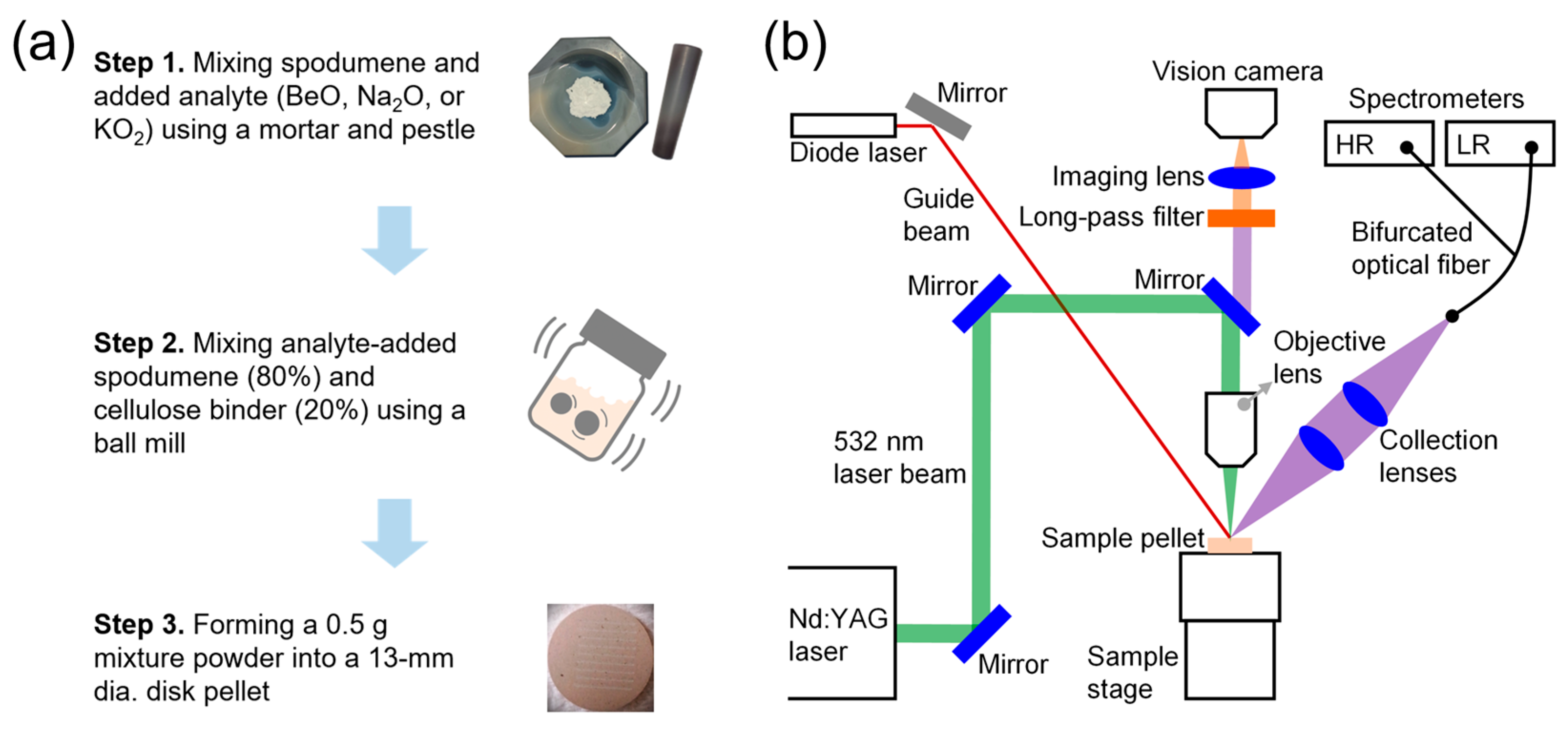
To determine the concentration of Be in the pristine spodumene sample, the two Be II and Be I emission intensities at 313.06 and 332.12 nm, respectively, were employed for the analyte signals. The Be II and Be I emission intensities were plotted with respect to the relative concentrations of Be and are shown in Figure 5a and Figure 5b, respectively. The relative concentration of 0 wt.% corresponds to the pristine spodumene sample. It should be noted that the dominant factor affecting sample uniformity lies in how well the spodumene and the added analyte compounds were mixed, which manifests as compositional inhomogeneity at the millimeter scale on the sample pellet surface. This effect is clearly illustrated in the calibration curves based on the Be II (313.06 nm) and Be I (332.12) nm emission peak intensities. Notably, the standard deviation of emission intensities in the unspiked spodumene sample (0 wt.% Be) is significantly smaller than those in the spiked samples. This observation indicates that the initial mixing step (Step 1) of spodumene with analyte compounds in the LIBS sample preparation process (Figure 1b) plays the most critical role in determining sample uniformity. In our LIBS analysis, nine line-scans were performed over a 7 mm × 9 mm area on the surface of a 13 mm-diameter pellet, and the averaged data were used for quantification. This averaging process helps mitigate the effect of millimeter-scale inhomogeneity caused by incomplete mixing, allowing us to obtain representative bulk composition values, although the incomplete mixing definitely decreased the precision performance. The measured intensities were fitted well to a linear function, y = a + bx, where y and x represent the emission intensity and the relative concentration, respectively. The coefficients of determination, R², were 0.990 and 0.989 for the linear fits of the Be II and Be I emission intensities, respectively. Following the principle of the standard addition method, the concentration of Be in the pristine spodumene samples was determined by calculating the concentration value corresponding to the zero intensity, y = 0 [27]. Thus, the concentration of Be in the pristine sample was calculated using the following equation.

$${\left|x\right|}_{y=0}=a/b$$

(1)

In the above equation, a and b are the intercept and the slope determined by the linear fits. Fitting the two Be emission peaks, however, led to remarkably different concentrations of Be in the pristine spodumene. The concentrations, 1390 ± 130 and 215 ± 30 mg/kg, were obtained from fitting the Be II and Be I emission intensities, respectively. As mentioned in the Materials and Methods Section, the concentrations of Be, Na, and K in the pristine spodumene were determined by ICP-OES prior to LIBS analysis. From the ICP-OES analysis, the Be concentration in the pristine spodumene was determined to be 253 ± 13 mg/kg. The analyte concentrations determined by LIBS and ICP-OES are listed in

Table 2. Concentrations of Be, Na, and K determined by LIBS and ICP-OES.

Element	Emission Line for LIBS Analysis	Concentration (mg/kg) LIBS	Concentration (mg/kg) ICP-OES	Relative Error (%)
Be	Be I 332.13 nm	215 ± 30	253 ± 13	15
	Be II 313.04 nm	1390 ± 130		450
Na	Na I 819.48 nm	3000 ± 140	2660 ± 130	13
	Na I 330.24 nm	4340 ± 570		63
K	K I 766.48 nm (Tail)	3060 ± 480	3240 ± 160	5.5
	K I 766.48 nm	16,800 ± 1400		420

.

Comparing the two LIBS results with those from ICP-OES, the Be I emission peak was found to provide a more accurate result with a relative error of 15%. However, the stronger Be II emission peak showed remarkable deviation from the ICP-OES result. The failure of the stronger Be II emission peak to determine the Be concentration in the pristine spodumene using the standard addition method can be understood by investigating the spectroscopic parameters listed in Table 1. One of the drawbacks in the application of the standard addition method to LIBS analysis is the varying sensitivity of LIBS signal intensities to the analyte concentration. Generally, the sensitivity in LIBS analysis shows linearity in the concentration region much narrower than those of other techniques such as ICP-OES, ICP-MS, and AAS. This is mainly due to self-absorption that is the re-absorption of the light emitted from the hot plasma core passing through the cold periphery of the plasma [29]. It should be noted that the lower energy level of the Be II emission is the ground state, whereas, for the Be I emission, it is an excited state that can further relax to lower or ground states (see the parameters listed in Table 1). The emission lines with zero lower-level energy like that of Be II at 313.06 nm, called “resonance lines”, are much more labile to the self-absorption because they have no other way than re-absorption after emission. On the other hand, the non-resonance lines like that of Be I at 332.12 can suppress the self-absorption effect on their emission intensities by relaxing further down to the lower levels [29]. In addition to the lower-level energy, the spontaneous emission coefficients should be compared between the Be II and Be I emissions. There is a proportional relationship between the spontaneous emission and absorption coefficients, A_ki and B_ik, respectively, as shown below.

$$A_{\mathrm{ki}}={\displaystyle \frac{8\pi h{\nu }^3}{c^3}}{\displaystyle \frac{g_{\mathrm{i}}}{g_{\mathrm{k}}}}{B}_{\mathrm{ik}}$$

(2)

In the above equation, h, ν, c, and g_i indicate Planck’s constant, the frequency of the emitted light, the speed of light, and the statistical weight of the lower level, respectively. This equation indicates that the stronger emission line is more sensitive to self-absorption due to the larger absorption coefficient proportional to the spontaneous emission coefficient [30]. Although the Be II and Be I emission peaks are composed of a few closely spaced lines, the Be II peak contains the lines with larger spontaneous emission coefficients than those of the lines in the Be I peak. This indicates that the Be II emission peak intensity is more strongly influenced by the self-absorption than that of Be I. Also, the self-absorption effect becomes stronger when the analyte concentration is higher [29]. As a result, the emission intensity is decreased more by the re-absorption as the analyte concentration goes higher. This makes the sensitivity of the emission intensity to the analyte concentration lower in the higher concentrations. Considering these factors related to the self-absorption effect, the low accuracy of fitting the Be II emission intensities in determining the Be concentration can be attributed to the slope, b, that is too small due to the self-absorption.

It should be noted that larger fluctuations in the intensities of Be compared to Na are observed, although the experiment is performed under similar conditions (see the following Figure 6). This shows that Be is more sensitive to the plasma conditions (plasma temperatures and densities) that vary with the shot-to-shot variations in the laser energy. This is supported by the fact that the ionization potential of Be (9.32 eV) is much higher compared to the ionization potential of Na (5.1 eV). Thus, small variations in laser energies may result in a large difference in the number of electrons detached from the Be atom. To improve measurement precision, we also investigated the effect of internal standardization by normalizing the Be I emission intensity at 332.13 nm with the Al I emission at 308.22 nm. Although this approach significantly reduced the RSD, it compromised sensitivity due to potential self-absorption in the reference line. As the standard addition method prioritizes sensitivity to ensure accurate calibration slopes, the raw Be I intensity yielded a Be concentration closer to the ICP-OES result. Therefore, in the following, we focused on selecting analyte lines that provide both high sensitivity and minimal self-absorption, rather than applying internal standardization.

3.3. Quantification of Na

To determine the concentration of Na in the pristine spodumene sample, the two Na I emission intensities at 330.24 and 819.48.12 nm were employed for the analyte signals. The Na I emission intensities were plotted with respect to the relative concentrations of Na and are shown in Figure 6a and Figure 6b, respectively. The intensities of both Na I emission peaks were fitted well using a linear function, and the R² values are noted in the corresponding panels of Figure 6. The concentration of Na in the pristine spodumene was calculated as the ratio of the fitted parameters, a/b. Fitting the intensities of the Na I emission peak at 330.24 nm resulted in the Na concentration of 4340 ± 570 mg/kg. Comparing this result with the Na concentration determined by ICP-OES, 2660 ± 130 mg/kg, the relative error was estimated to be 63%. On the other hand, using the Na I emission peak at 819.48 nm, the Na concentration was determined to be 3000 ± 140 mg/kg, which agreed with the result from ICP-OES within 13% relative error. To rationalize the better accuracy of the Na I emission peak at 819.48 nm, it should be noted that the peak at 819.48 nm is composed of non-resonance lines (see the spectroscopic parameters listed in Table 1). Thus, the emission intensities could not be affected by the self-absorption. However, the peak intensity at 330.24 nm is contributed by two resonance lines. The larger Na concentration value from fitting the Na I peak intensities at 330.24 nm than that from ICP-OES can be attributed to the decreased sensitivity by the self-absorption effect on the measured intensities.

Both of the Na I emission peak intensities at 330.24 nm and 819.48 nm showed comparable RSDs of 3.8% and 4.2%, respectively. These RSD values are the average of the RSDs of the five measurement groups with the spodumene samples spiked with 0, 0.2, 0.4, 0.6, and 0.8 wt.% of added Na. It is important to note that, in principle, RSD and signal-to-noise ratio (SNR) are not significantly influenced by whether the corresponding emission line is a resonance or a non-resonance line. Rather, it is the sensitivity—not the precision—that is affected by the resonance characteristics of the emission line. Accordingly, the measurement precision, as reflected by the RSD, was similar between the resonance Na I line at 330.24 nm and the non-resonance Na I line at 819.48 nm. In contrast, the Be II emission at 313.04 nm exhibited a higher RSD of 47%, while the Be I emission at 332.13 nm showed an RSD of 39%. This discrepancy can be attributed to the particularly high ionization potential of Be (9.32 eV), as mentioned earlier. The formation of the ionic species Be II requires higher plasma temperatures, making its signal more susceptible to plasma temperature fluctuations. This results in greater uncertainty in intensity measurements compared to the atomic species Be I.

3.4. Quantification of K

As mentioned above, K I emission lines were observed around 404.5 and 768 nm. The K I emission lines around 404.5 nm may be more appropriate for the standard addition method because their intensities are much weaker than those around 768 nm. However, they were interfered with by the Fe I emission line at 404.58 nm (see Figure 3c). The spectral interference would make the standard addition method inaccurate due to uncertainty in setting the baseline of the analyte signal. The analyte concentration is determined from the parameters a and b, fitted using a linear function as a/b. The parameter a is the analyte signal corresponding to the pristine sample. However, a can be overestimated if the analyte signal is interfered with by other nearby emissions and if the baseline is not properly subtracted. This would lead to overestimation of the analyte concentration even though the sensitivity, b, has been measured accurately. The strong K I emission line at 766.49 nm was thus chosen for the analyte signal. This resulted in the ratio, a/b, corresponding to 16,800 ± 1400 mg/kg, which is too large to be accepted as the concentration of K in the pristine spodumene sample (3240 ± 160 mg/kg). The cause of the large deviation in the determined K concentration can be attributed to the decreased sensitivity due to the self-absorption of the strong and resonant K I emission line (see A_ki and E_i values listed in Table 1). Whether the K I emission line intensities at 766.49 and 769.90 nm were affected by the self-absorption or not can be checked by investigating the intensity ratio of them. When their intensities are free from the self-absorption, the ratio of the K I line intensity at 766.49 nm to that at 769.90 nm is estimated to be ~2:1 considering their spectroscopic parameters listed in Table 1. The two emission lines have very similar spectroscopic parameters other than g_k. The g_k value of the K I emission line at 766.49 nm is 4, twice of that at 769.90 nm. The observed ratio of the K I emission line intensity at 766.49 nm to that at 769.90 nm is 1.6:1. This definitely indicates that the K I emission line intensities were affected by the self-absorption. The stronger one of the two lines was affected by the self-absorption more severely. Thus, the intensity ratio decreased from 2:1 to 1.6:1.

Inspired by Equation (2), which indicates that weaker emissions are less re-absorbed, the accuracy of fitting the edge intensities of the K I peak emission profile was investigated in the following. This approach is supported by the mechanism of the self-absorption that becomes more severe in the center of the spectral line profile than in the wings [29]. The expanded spectra around 765.5 nm in Figure 7 shows the profile of the K I emission line centered at 766.49 nm for the spodumene samples to which different amounts of KO₂ were added. The relative concentrations of K were noted in the panel of Figure 6. The emission intensities measured at 766.48, 765.92, 765.35, 764.78, 764.21, 763.65, and 763.08 nm are represented by I₁, I₂, I₃, I₄, I₅, I₆, and I_B. Among them, the intensity at 763.08 nm, I_B, was taken as the baseline intensity.

Thus, the six calibration curves shown in Figure 8 were constructed using the baseline-subtracted intensities—Figure 8a I₁ − I_B, Figure 8b I₂ − I_B, Figure 8c I₃ − I_B, Figure 8d I₄ − I_B, Figure 8e I₅ − I_B, and Figure 8f I₆ − I_B. The baseline subtraction is also crucial to obtain accurate results from the standard addition method because the analyte concentration is calculated as a/b. This indicates that the analyte concentration can be overestimated when the baseline is not completely subtracted from the measured intensities. Herein, any possible spectral interference to the K I emission line at 766.49 nm was not identified, and thus the baseline, I_B, seems to be due to continuum background emission. The wavelength shift from the center of the K I emission line at 766.49 nm to the blue side, ∆λ, increases from I₁ to I₆ and simultaneously the emission intensity value also decreases. Thus, the self-absorption effect becomes weaker as ∆λ increases. In Figure 8, the red solid lines are the linear fits of the baseline-subtracted intensity values, and the red dashed lines are the extrapolation to the relative concentration values corresponding to the zero intensities. From the fitted parameters, a and b, the ratio values of a/b were calculated and noted in the corresponding panels. As expected from considering the self-absorption effect, the intensity values, I₆ − I_B, at the furthest edge of the K I line profile provided the most accurate K concentration values, (a/b) × 10,000 = 3060 ± 480 mg/kg, leading to the error of 5.5% from the ICP-OES result, 3240 ± 160 mg/kg.

The predicted K concentrations, obtained by fitting I₁ − I_B, I₂ − I_B, I₃ − I_B, I₄ − I_B, I₅ − I_B, and I₆ − I_B, show a systematic trend with Δλ. Figure 9a shows the (a/b) × 10,000 values from the six calibration curves from LIBS, corresponding to the K concentrations in mg/kg, with respect to Δλ along with the ICP-OES result. As the wavelength at which the intensities were taken for the calibration curve of the standard addition method was shifted toward the blue-side edge, the K concentration approached more closely to the ICP-OES result. This can be rationalized by the decreased self-absorption effect on the weaker edge emission intensities and justified by the increased sensitivity of the emission intensity to the K concentration. The six calibration curves shown in Figure 8 exhibit a decrease in the slope of the linear fit from I₁ − I_B to I₆ − I_B. The fitted parameter b, corresponding to the slope, cannot be directly compared among the six calibration curves because the baseline-subtracted intensities differ significantly among them. To compare the sensitivities obtained from signals measured at the different intensity levels, it is necessary to introduce the concept of “% sensitivity”. Sensitivity refers to the ability of a method or instrument to detect small changes in analyte concentration. It is generally defined as the slope of the calibration curve, ΔI/Δc, where ΔI and Δc are changes in the signal intensity and the analyte concentration, respectively. In addition, % sensitivity uses the % change in the signal intensity, Δ%I, in place of ΔI. The % change in the signal intensity can be estimated as below.

$$∆\%I={\displaystyle \frac{I_{\max }-I_{\min }}{\begin{array}{c}{I}_{\max }\end{array}}}\times 100\%$$

(3)

In the above equation, I_max and I_min represent the measured intensities for the standards with the maximum and minimum analyte concentrations. Herein, I_max and I_min represent the K I emission intensities for the spodumene samples to which KO₂ compounds were added to achieve the relative concentration of K 0.8 and 0 wt.%, respectively. Then, the % sensitivity values were calculated as Δ%I/Δc with Δc = (0.8 − 0.0) wt.% and noted in the corresponding panels of Figure 8. As expected due to the self-absorption effect, which is more pronounced for stronger emissions and higher analyte concentrations, the % sensitivity increases for the weaker edge emission intensities. The weakest emission intensity, I₆ − I_B, exhibits a 72.3% decrease as the K concentration decreases from 0.8 to 0.0 wt.%. This is the most sensitive change in the emission intensity among the six analyte signals I₁ − I_B, I₂ − I_B, I₃ − I_B, I₄ − I_B, I₅ − I_B, and I₆ − I_B. The strongest analyte signal, I₁ − I_B, showed a % sensitivity of 35.5%, which is much smaller than that of the weakest analyte signal, I₆ − I_B.

It should be noted that while a weaker signal is preferred to achieve accurate results in the standard addition method, it is disadvantageous for precision. This is well demonstrated in Figure 9b. The blue-filled squares in Figure 9b represent the relative standard deviation of the K concentration determined by fitting the baseline-subtracted K I emission intensities, I₁ − I_B, I₂ − I_B, I₃ − I_B, I₄ − I_B, I₅ − I_B, and I₆ − I_B, that were taken at the wavelengths shifted toward the blue side by Δλ = 0.10, 0.57, 1.14, 1.71, 2.28, and 2.84 nm, respectively. Although the relative standard deviation decreases from Δλ = 0.10 to 1.14 nm, it increases afterward and the weakest analyte signal at Δλ = 2.84 nm shows the largest standard deviation. However, the relative error, indicated by the red-filled squares in Figure 9b, decreases as Δλ increases. This observation suggests that accuracy and precision do not always improve concurrently, particularly when weak emission signals are used. As Δλ increases, the edge intensity becomes weaker, which leads to a higher sensitivity in the calibration curve and thus improves the accuracy of the standard addition method, as reflected in the decreasing relative error. However, the relative standard deviation increases for these weaker signals because it is calculated as the ratio of the standard deviation to the mean intensity. While the absolute fluctuation in signal intensity may remain similar, the average intensity becomes smaller as weaker edges are used, resulting in a larger RSD. Therefore, although the use of edge intensities effectively enhances analytical accuracy by mitigating self-absorption effects, it imposes a trade-off in terms of decreased precision. This explains the diverging trends of relative error and relative standard deviation in Figure 9b, even though both metrics were derived from the same measurement data.

Finally, we compared our results with previously reported concentrations of Be, Na, and K in various spodumene samples. These concentrations vary depending on the spodumene type and the geological setting of the deposits [8,31,32,33]. Göd et al. analyzed spodumene from Weinebene, Austria and reported Na₂O (2.07–4.74 wt.%), K₂O (1.20–5.58 wt.%), and Be (11–110 ppm) in amphibolite-hosted pegmatites, and Na₂O (1.20–5.58 wt.%), K₂O (1.99–2.71 wt.%), and Be (41–68 ppm) in micaschist-hosted pegmatites [31]. Fosu et al. used Mineral Liberation Analysis to assess spodumene concentrates from Li-Cs-Ta-type pegmatites, reporting K and Na concentrations of 1.34 wt.% and ~0.76 wt.%, respectively, and compared results with energy-dispersive X-ray spectroscopy (EDS), XRF, and ICP-OES [32]. Wang et al. found Na (818–3139 ppm), K (12.2–1682 ppm), and Be (4.11–15.4 ppm) in spodumene pegmatites from Lhozhag, eastern Himalaya [8]. Skublov et al. examined impurity element zoning in colorless beryl from spodumene pegmatites in the Pashki deposit, Afghanistan, and reported Na (6591–8879 ppm) and K (511–910 ppm) [33]. In line with these findings, our data also show relatively high concentrations of Na and K (3000 ± 140 mg/kg and 3040 ± 480 mg/kg, respectively) and significantly lower concentrations of Be (253 ± 13 mg/kg).

4. Conclusions

In this study, we evaluated the feasibility of combining LIBS with the standard addition method for the accurate and rapid analysis of impurity elements, specifically Be, Na, and K, in spodumene samples. Our findings demonstrate that this approach can provide reliable results without reliance on matrix-matched standard materials, overcoming the disadvantages of conventional techniques like ICP-OES and XRF, which require extensive sample preparation and limited accessibility to light elements such as Be and Na. The results show that using non-resonance emissions for Be and Na enables accurate quantification by reducing the self-absorption effect, achieving relative errors within 5%–15% compared to ICP-OES results. For K, despite challenges posed by strong resonance emissions and significant self-absorption, accuracy was markedly improved by focusing on the weaker blue-side edge emissions. This approach reduced the relative error in K concentration from 420% to 5.5%, highlighting the potential of weak edge emissions in circumventing self-absorption. Overall, LIBS combined with the standard addition method emerges as a promising alternative to traditional methods for the multi-elemental analysis of lithium-bearing minerals. The technique’s simplicity, requiring no acid digestion or dilution, along with its capacity for simultaneous detection of light and heavy elements, offers considerable advantages in industrial applications, especially in settings where quick, on-site analysis is needed. These benefits position this method as a valuable tool for supporting the rapid and efficient processing of lithium ores, aligning with the growing demand in the energy storage sector. Future work will explore the broader applicability of this approach across different mineral matrices to enhance its robustness and expand its practical utility. Given the critical importance of lithium minerals in the supply chain of the lithium-ion battery industry, analytical techniques capable of providing rapid and reasonably accurate results are essential. The method proposed in this study can yield analytical results, including sample preparation, within a few hours. Compared to ICP-OES, which requires prolonged acid digestion and separate analyses for certified reference materials, the proposed LIBS-based method offers significantly faster turnaround times. For even more rapid on-site analysis, the feasibility of performing LIBS directly on powdered samples without pelletizing with a binder would be highly advantageous. In such cases, the standard addition method could still be applicable to account for matrix effects. Our research group is currently conducting studies on direct LIBS analysis of lithium ore powders to further enhance the field applicability of this technique.

References

1. Bibienne, T.; Magnan, J.-F.; Rupp, A.; Laroche, N. From mine to mind and mobiles: Society’s increasing dependence on lithium. Elements 2020, 16, 265–270. [Google Scholar] [CrossRef]
2. Publications Office of the European Union, EU. Study on the EU’s List of Critical Raw Materials. 2020. Available online: https://op.europa.eu/en/publication-detail/-/publication/c0d5292a-ee54-11ea-991b-01aa75ed71a1/language-en (accessed on 12 December 2024).
3. U.S. Government Publishing Office, Virginia, USA. Mineral Commodity Summaries. 2020. Available online: https://pubs.usgs.gov/publication/mcs2020 (accessed on 12 December 2024).
4. Brennan, C.J.; Student, J.J.; Hill, T.; Martins, T.; Sirbescu, M.L.C. Trace element concentrations and chemical zoning of spodumene from magmatic and hydrothermal origins. Ore Geol. Rev. 2024, 169, 106089. [Google Scholar] [CrossRef]
5. Sirbescu, M.L.C.; Doran, K.; Konieczka, V.A.; Brennan, C.J.; Kelly, N.M.; Hill, T.; Knapp, J.; Student, J.J. Trace element geochemistry of spodumene megacrystals: A combined portable-XRF and micro-XRF study. Chem. Geo. 2023, 621, 121371. [Google Scholar] [CrossRef]
6. Gourcerol, B.; Gloaguen, E.; Melleton, J.; Tuduri, J.; Galiegue, X. Re-assessing the European lithium resource potential—A review of hard-rock resources and metallogeny. Ore Geol. Rev. 2019, 109, 494–519. [Google Scholar] [CrossRef]
7. D’yachkov, B.A.; Bissatova, A.Y.; Mizernaya, M.A.; Khromykh, S.V.; Oitseva, T.A.; Kuzmina, O.N.; Zimanovskaya, N.A.; Aitbayeva, S.S. Mineralogical tracers of gold and rare-metal mineralization in eastern Kazakhstan. Minerals 2021, 11, 253. [Google Scholar] [CrossRef]
8. Wang, J.M.; Hou, K.S.; Yang, L.; Liu, X.C.; Wang, R.C.; Li, G.M.; Fu, J.G.; Hu, F.Y.; Tian, Y.L.; Wu, F.Y. Mineralogy, petrology and P-T conditions of the spodumene pegmatites and surrounding meta-sediments in Lhozhag, eastern Himalaya. Lithos 2023, 456–457, 107295. [Google Scholar] [CrossRef]
9. Czaja, M.; Lisiecki, R.; Kądziołka-Gaweł, M.; Winiarski, A. Some complementary data about the spectroscopic properties of manganese ions in spodumene crystals. Minerals 2020, 10, 554. [Google Scholar] [CrossRef]
10. Ito, A.S.; Isotani, S. Heating effects on the optical absorption spectra of irradiated, natural spodumene. Radiat. Eff. Defects Solids 1991, 116, 307–314. [Google Scholar] [CrossRef]
11. Rehman, H.U.; Martens, G.; Tsai, Y.L.; Chankhantha, C.; Kidkhunthod, P.; Shen, A.H. An X-ray absorption near-edge structure (XANES) study on the oxidation state of chromophores in natural nunzite samples from Nuristan, Afghanistan. Minerals 2020, 10, 463. [Google Scholar] [CrossRef]
12. Sardisco, L.; Hannula, P.-M.; Pearce, T.J.; Morgan, L. Multi-technique analytical approach to quantitative analysis of spodumene. Minerals 2022, 12, 175. [Google Scholar] [CrossRef]
13. Fabre, C.; Ourti, N.E.; Ballouard, C.; Mercadier, J.; Cauzid, J. Handheld LIBS analysis for in situ quantification of Li and detection of the trace elements (Be, Rb and Cs). J. Geochem. Explor. 2022, 236, 106979. [Google Scholar] [CrossRef]
14. Bertin, E.P. Principles and Practice of X-Ray Spectrometric Analysis; Plenum Press: New York, NY, USA, 1970. [Google Scholar]
15. Yi, R.X.; Guo, L.B.; Zou, X.H.; Li, J.M.; Hao, Z.Q.; Yang, X.Y.; Li, X.Y.; Zeng, X.Y.; Lu, Y.F. Background removal in soil analysis using laser-induced breakdown spectroscopy combined with standard addition method. Opt. Express 2016, 24, 2607–2618. [Google Scholar] [CrossRef] [PubMed]
16. Svanberg, S. Laser spectroscopy in medical diagnostics. In Lasers for Medical Applications, 1st ed.; Jelínková, H., Ed.; Woodhead Publishing: Cambridge, UK, 2013; pp. 286–318. [Google Scholar]
17. Clegg, S.M.; Sklute, E.; Dyar, M.D.; Barefield, J.E.; Wiens, R.C. Multivariate analysis of remote laser-induced breakdown spectroscopy spectra using partial least squares, principal component analysis, and related techniques. Spectrochim. Acta B 2009, 64, 79–88. [Google Scholar] [CrossRef]
18. Umar, Z.A.; Liaqat, U.; Ahmed, R.; Baig, M.A. Detection of lead in soil implying sample heating and laser-induced breakdown spectroscopy. Appl. Opt. 2021, 60, 452–458. [Google Scholar] [CrossRef]
19. Kumar, S.; Park, J.; Singh, V.K.; Nam, S.-H.; Yoo, C.-Y.; Lee, Y. Univariate and multivariate analyses of Gd in gadolinia-doped ceria using laser-induced breakdown spectroscopy. Optik 2021, 240, 166909. [Google Scholar] [CrossRef]
20. Gondal, M.A.; Hussain, T.; Ahmed, Z.; Bakry, A.H. Detection of contaminants in ore samples using laser-induced breakdown spectroscopy. J. Environ. Sci. Health A Tox. Hazard Subst. Environ. Eng. 2007, 42, 879–887. [Google Scholar] [CrossRef]
21. Bilge, G.; Eseller, K.E.; Berberoglu, H.; Sezer, B.; Tamer, U.; Boyaci, I.H. Comparison of different calibration techniques of laser induced breakdown spectroscopy in bakery products on NaCl measurement. J. Eur. Opt. Soc.-Rapid Publ. 2021, 17, 18. [Google Scholar] [CrossRef]
22. Bhatt, C.R.; Hartzler, D.; McIntyre, D. LIBS sensing for in-situ iron detection and quantification in wastewater outfall. Appl. Phys. B 2024, 130, 18. [Google Scholar] [CrossRef]
23. Kumar, S.; Park, J.; Yoo, C.-Y.; Nam, S.-H.; Lee, Y. Quantitative analysis of ceria co-doped with samarium and gadolinium using laser-induced breakdown spectroscopy. Anal. Methods 2022, 14, 597–605. [Google Scholar] [CrossRef]
24. Kim, H.; Nam, S.-H.; Han, S.-H.; Jung, S.; Lee, Y. Laser-induced breakdown spectroscopy analysis of alloying elements in steel: Partial least squares modeling based on the low-resolution spectra and their first derivatives. Opt. Laser Technol. 2019, 112, 117–125. [Google Scholar] [CrossRef]
25. Kim, Y.S.; Han, B.Y.; Shin, H.S.; Kim, H.D.; Jung, E.C.; Jung, J.H.; Na, S.H. Determination of uranium concentration in an ore sample using laser-induced breakdown spectroscopy. Spectrochim. Acta B 2012, 74–75, 190–193. [Google Scholar] [CrossRef]
26. Singh, J.; Kumar, R.; Awasthi, S.; Singh, V.; Rai, A.K. Laser Induced breakdown spectroscopy: A rapid tool for the identification and quantification of minerals in cucurbit seeds. Food Chem. 2017, 221, 1778–1783. [Google Scholar] [CrossRef] [PubMed]
27. Skoog, D.A.; Holler, J.F.; Crouch, S.R. Principles of Instrumental Analysis, 6th ed.; Cengage Learning: Boston, MA, USA, 2007. [Google Scholar]
28. The National Institute of Standards and Technology (NIST). NIST Atomic Spectra Database. 2012. Available online: http://www.nist.gov/pml/data/asd.cfm (accessed on 15 June 2024).
29. Tang, Y.; Liao, P.; Yang, K.; Hu, Z.; Zhang, D.; Yang, Z.; Wang, S.; Guo, E.; Zhao, N. A review of development in the research of self-absorption on laser-induced breakdown spectroscopy. At. Spectrosc. 2024, 45, 336–357. [Google Scholar] [CrossRef]
30. Thakur, S.N. Atomic Emission Spectroscopy. In Laser-Induced Breakdown Spectroscopy; Singh, J.P., Thakur, S.N., Eds.; Elsevier Science: Amsterdam, The Netherlands, 2007; pp. 36–37. [Google Scholar]
31. Göd, R. The spodumene deposit at “Weinebene”, Koralpe, Austria. Mineral. Deposita 1989, 24, 270–278. [Google Scholar] [CrossRef]
32. Fosu, A.Y.; Kanari, N.; Bartier, D.; Hodge, H.; Chagnes, J.V.A. Physico-chemical characteristics of spodumene concentrate and its thermal transformations. Materials 2021, 14, 7423. [Google Scholar] [CrossRef]
33. Skublov, S.G.; Hamdard, N.; Ivanov, M.A.; Stativko, V.S. Trace element zoning of colorless beryl from spodumene pegmatites of Pashki deposit (Nuristan province, Afghanistan). Front. Earth Sci. 2024, 12, 1432222. [Google Scholar] [CrossRef]
Figure 1. Schematic diagram of (a) the LIBS sample preparation process and (b) the LIBS setup. In (b), “HR” and “LR” stand for “high-resolution” and “low-resolution”, respectively.
Minerals 15 00659 g001
Figure 2. Normalized SNR values of Na I (330 nm) and Be II (313 nm) emission peak intensities with respect to the detection gate delay time from the laser Q-switching.
Minerals 15 00659 g002
Figure 3. (a) A high-resolution LIBS spectrum of the unspiked spodumene mixed with cellulose binder without adding any analyte compounds in the wavelength region between 302 and 407 nm; (b) a low-resolution LIBS spectrum of spodumene without adding any compounds in the wavelength region between 775 and 830 nm; and (c) the expanded spectrum of the high-resolution spectrum shown in the wavelength region between 403.7 and 405.0 nm. The emission peaks marked with “*” in a and b were employed for the analyses in this work.
Minerals 15 00659 g003
Figure 4. Variations in the emission intensities measured for the spodumene samples to which (a) BeO, (b,c) Na2O, and (d) KO2 were added.
Minerals 15 00659 g004
Figure 5. Calibration curves for the standard addition method to determine the Be concentration in the spodumene sample. The intensities of the (a) Be II and (b) Be I emission lines at 313.04 and 332.13 nm, respectively, were used for the calibration curves. The calibration curves (solid lines) are extrapolated below 0 wt. % of the relative concentration of Be (dashed lines) to find the intercept with the horizontal axis corresponding to −a/b values noted in the panels.
Minerals 15 00659 g005
Figure 6. Calibration curves for the standard addition method to determine the Na concentration in the spodumene sample. The intensities of the Na I emission lines at (a) 330.24 and (b) 819.48 nm were used for the calibration curves. The calibration curves (solid lines) are extrapolated below 0 wt. % of the relative concentration of Na (dashed lines) to find the intercept with the horizontal axis corresponding to −a/b values noted in the panels.
Minerals 15 00659 g006
Figure 7. The K I emission line profile centered at 766.49 nm. I1, I2, I3, I4, I5, I6, and IB represent the intensities measured at 766.48, 765.92, 765.35, 764.78, 764.21, 763.65, and 763.08 nm, respectively.
Minerals 15 00659 g007
Figure 8. Calibration curves for the standard addition method. The baseline-subtracted intensities, (a) I1IB, (b) I2IB, (c) I3IB, (d) I4IB, (e) I5IB, and (f) I6IB, were used for the calibration curves. The emission intensities I1, I2, I3, I4, I5, I6, and IB were taken at 766.48, 765.92, 765.35, 764.78, 764.21, 763.65, and 763.08 nm, respectively, and IB was used for the baseline intensity. The calibration curves (solid lines) are extrapolated below 0 wt. % of the relative concentration of K (dashed lines) to find the intercept with the horizontal axis corresponding to −a/b values noted in the panels.
Minerals 15 00659 g008
Figure 9. (a) The (a/b) × 10,000 values, corresponding to the K concentrations in mg/kg determined by the standard addition method using the edge emission intensities of the K I line at 766.49 nm, with respect to the shift from the center wavelength to the blue side, Δλ, and (b) relative standard deviations and relative errors of the K concentrations with respect to Δλ. The horizontal dashed line indicates the K concentration determined by ICP-OES.
Minerals 15 00659 g009