Unsupervised Anomaly Detection for Mineral Prospectivity Mapping Using Isolation Forest and Extended Isolation Forest Algorithms

Abstract

Unsupervised anomaly detection algorithms have gained significant attention in the field of mineral prospectivity mapping (MPM) due to their ability to reveal hidden mineralization zones by effectively modeling complex, nonlinear relationships between exploration data and mineral deposits. This study utilizes two tree-based anomaly detection algorithms, namely, isolation forest (IF) and extended isolation forest (EIF), to enhance MPM and exploration targeting. According to the conceptual model of porphyry copper deposits, several evidence layers were generated, including fault density, multi-element geochemical signatures, proximity to various alteration types (phyllic, argillic, propylitic, and iron oxide), and proximity to intrusive rocks. These layers were integrated using IF and EIF algorithms, and their results were subsequently compared with a geological map of the study area. The comparison revealed a high degree of overlap between the identified anomalous zones and geological features, such as andesitic rocks, tuffs, rhyolites, pyroclastics, and intrusions. Additionally, quantitative assessments through prediction-area plots validated the efficacy of both models in generating prospective targets. The results highlight the significant influence of hyperparameter tuning on the accuracy of prospectivity models. Furthermore, the study demonstrates that hyperparameter tuning is more intuitive and straightforward in IF, as it provides a clear and distinct tuning pattern, whereas EIF lacks such clarity, complicating the optimization process.

1. Introduction

In recent decades, mineral deposits with strong geochemical, geophysical, and geological footprints have been widely explored and extracted and are close to depletion. Meanwhile, advancements in industry and technology have led to a substantial increase in the demand for mineral resources. As a result, it’s become crucial to use more efficient and precise methods for identifying promising mineralization areas with minimal footprints in geochemical or geophysical data. Moreover, relying solely on a single type of exploration dataset might lead to missing some exploration targets due to limited coverage or incomplete datasets. Consequently, integrating multi-disciplinary spatial datasets through mineral prospectivity mapping (MPM) [1,2] frameworks can be an effective approach for identifying promising areas and enhancing the accuracy of discovering new mineralization zones [3,4,5]. MPM is a multi-stage analytical workflow [6,7] that integrates geo-exploration datasets to produce predictive models [8] and quantitatively assess the likelihood of mineralization within the study area [9]. This approach can be applied at various scales, from regional [10] to local [11], to identify areas with high mineralization potential [12]. MPM deals with multi-dimensional datasets that include various types of exploration data, including geological, geochemical, geophysical, and remote sensing information [13,14,15,16]. Creating multi-disciplinary geospatial datasets leads to complex, high-dimensional, and non-linear exploratory datasets that are challenging to process and integrate effectively using classical methods [8,17].

Various mathematical approaches have been used to implement MPM, generally classified into three main categories: data-driven, knowledge-driven, and hybrid approaches [18,19]. Some studies have proposed data-driven machine learning (ML) and deep learning (DL) algorithms due to their ability to learn nonlinear features from complex geospatial datasets [2,12,20,21,22,23,24,25]. These algorithms are typically divided into supervised and unsupervised learning. Supervised algorithms use labeled data, which include known deposit and non-deposit locations, to learn the appropriate features. With the help of these training points (labeled data), supervised algorithms extract the complex relationships between evidence layers and mineralized and non-mineralized locations and then apply them to identify high-potential areas [21]. The most widely used algorithms include support vector machines (SVMs) [24,26], random forests (RFs) [27,28,29], logistic regressions [30], neural networks [31,32], and convolutional neural networks (CNNs) [33,34,35]. Although these algorithms are highly effective at learning complex, non-linear relationships, the small number of positive training points (mineral deposits) and the lack of ground truth negative points (non-mineralized areas) pose challenges for supervised data-driven approaches. These limitations have restricted their application in the majority of MPM studies [13,36,37]. These approaches are effective when significant amounts of labeled data are available, such as in brownfield environments. However, since mineralization is a rare geological phenomenon [38], it inevitably leads to insufficient positive training samples (mineralization areas). In contrast, unsupervised learning algorithms detect patterns and structures within data without the need for labeled samples or prior knowledge [12]. The most commonly used unsupervised algorithms include various clustering algorithms (e.g., K-means [19] and SOM [31]), restricted Boltzmann machines (RBMs) [39], isolation forests (IFs) [14,40,41], one-class SVMs (OC-SVMs) [42], and deep autoencoders (DAEs) [13,20].

Among the unsupervised data-driven methods, the IF algorithm [43] is computationally efficient and highly suitable for analyzing high-dimensional datasets, which are common in MPM and geochemical studies [27,41,44]. Its ability to work without labeled data makes it a suitable tool for integrating exploratory layers and identifying high-potential areas. The IF algorithm was originally developed to detect anomalies in large and high-dimensional datasets [43]. It separates samples by building random binary trees and isolating samples by selecting random features and choosing a threshold limit between the maximum and minimum values of the selected feature. The anomaly score is determined by the path length required to isolate samples, where shorter paths indicate a higher anomaly likelihood. The key idea is that anomalies are rare and have distinct characteristics, so they are separated and isolated faster [45]. Several MPM and multivariate geochemical studies have proposed the IF algorithm to detect areas with high mineralization potential and to detect anomalous patterns in exploration datasets [14,27,40,46]. However, the IF algorithm often has biases in the anomaly score assignment due to its axis-parallel cuts, which may reduce its effectiveness in accurately detecting anomalies or patterns linked to mineralization in complex, high-dimensional geospatial datasets. To mitigate this issue, the extended isolation forest (EIF) [46] was developed by enhancing its capability to capture more subtle and complex anomalies through an improved splitting criterion, i.e., non-axis-parallel cuts. The EIF reduces false positives by improving data splitting more accurately at the expense of a longer runtime [47]. Chenyi et al. (2023) conducted a comparative study on IF, EIF, and generalized IF for detecting multivariate geochemical anomalies [46]. Their results indicate that EIF is superior for identifying multivariate geochemical anomalies, particularly in complex geological settings, and it effectively detects mineralization-related anomalies.

In this study, the IF and EIF algorithms were employed to identify prospective areas and generate prospectivity models for porphyry copper mineralization in the 1:100,000 Jebal Barez geological sheet, situated within the Urumieh–Dokhtar metallogenic zone (UDMZ). To achieve this, seven evidence layers were generated based on the geological characteristics and the conceptual model of porphyry copper deposits. These layers include fault density, proximity to intrusive rocks, distances from argillic, phyllic, propylitic, and iron oxide alterations, and multi-element geochemical signatures. The optimal hyperparameter values for IF and EIF models were determined using the locations of known mineral deposits as ground truth points. The performance of the generated mineral potential models has been evaluated using the prediction-area (P-A) plot.

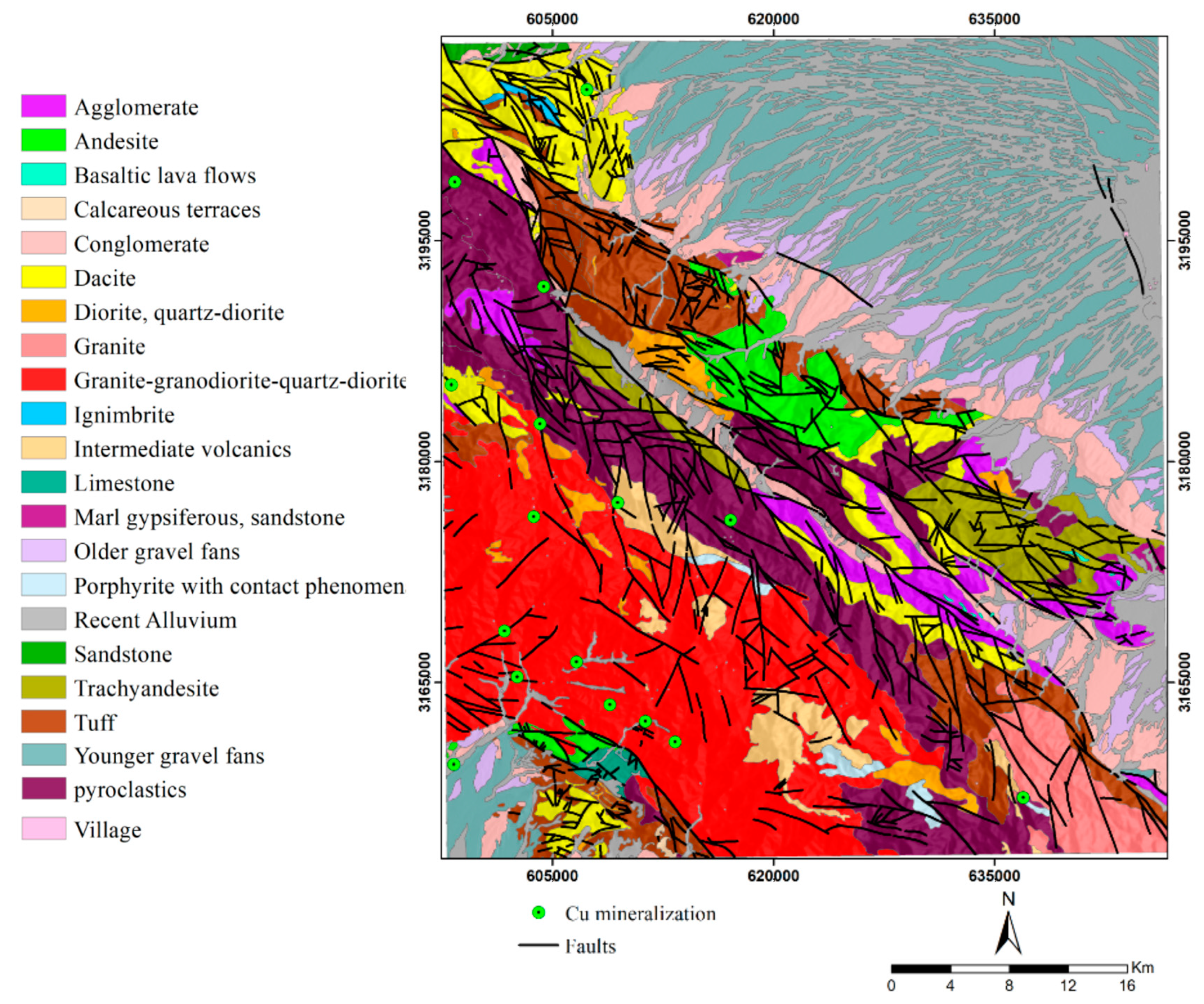
2. General Geological Setting of the Study Area

The closure of the Neo-Tethyan Ocean, along with the prevailing collisional tectonics during the Tertiary period, resulted in the formation of a significant metallogenic belt known as the Cenozoic UDMZ [48]. Most porphyry copper deposits in Iran are located within this belt, particularly in the Kerman metallogenic arc [49,50]. The Kerman Cenozoic magmatic arc is characterized by calc-alkaline intrusive rocks, which have facilitated extensive hydrothermal copper mineralization. The Jebal Barez geological map at a scale of 1:100000, covering approximately 2500 km² (Figure 1), is situated in the Kerman Cenozoic magmatic arc [51]. This geological region is characterized by favorable tectonic conditions and extensive hydrothermal alterations, indicating significant mineralization potential.

The presence of both oxide and sulfide mineralization indicators further highlights the high potential for metal deposit exploration [52]. The youngest lithological units in this region are dacitic rocks, formed by volcanic and plutonic activities. The Jebal Barez massif, which intrudes Eocene pyroclastic rocks, is likely dated to the late Eocene epoch. A significant number of dikes composed of diabase, pyroxene-diabase, diorite-micro-granodiorite, and alkaline granite have intruded the pyroclastic series and intrusive masses. Dykes are predominantly found in the eastern and western sections of the region, while the oldest exposed rocks are primarily situated in the northern part of the geological sheet. These rocks consist of folded sequences, characterized by dark gray to brownish-green calcareous sandstones interspersed with layers of shale, green marl, and conglomerate. The conglomerate has well-rounded, medium-to-coarse-sized fragments of Cretaceous limestones.

3. Raw Data and Creation of Evidence Layers

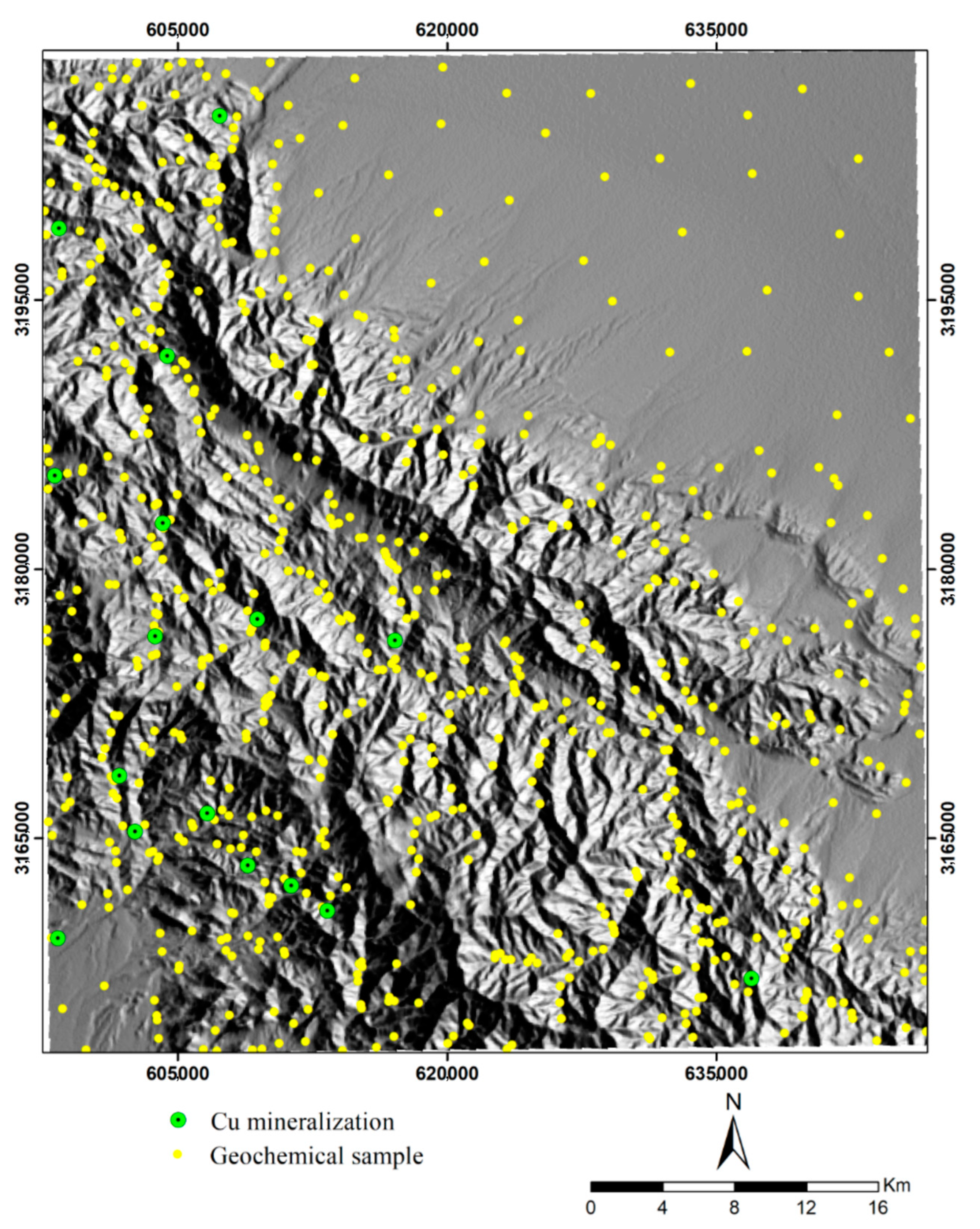
3.1. Remote Sensing and Geochemical Data

In recent decades, the processing of satellite imagery through statistical and mathematical methods has captured the attention of exploration geologists in mineral exploration tasks, providing a cost-effective tool for identifying surface footprints associated with various mineral deposit types [53,54,55,56]. In this study, an ASTER image (AST_L1T_00308092003065547_20150430104234_118405) was utilized to identify and map the distribution of hydrothermal alteration zones as a key indicator for the exploration of hydrothermal deposits, such as porphyry copper. The key characteristics of ASTER data are presented in

Table 1. Key characteristics of ASTER data.

Band	Spectral Region	Wavelength (µm)	Resolution (m)
B1	VNIR	0.520–0.60	15
B2		0.630–0.690
B3N		0.760–0.860
B3B		0.760–0.860
B4	SWIR	1.600–1.700	30
B5		2.145–2.185
B6		2.185–2.225
B7		2.235–2.285
B8		2.295–2.365
B9		2.360–2.430
B10	TIR	8.125–8.475	90
B11		8.475–8.825
B12		8.925–9.275
B13		10.250–10.950
B14		10.950–11.650

.

In addition to satellite data, this study utilized 745 stream sediment samples collected by the Geological and Mineral Exploration Survey of Iran to create a geochemical evidence layer. These samples were available for 20 elements (i.e., Zn, Pb, Ag, Cr, Ni, Bi, Sc, Cu, As, Sb, Cd, Co, Sn, Y, Ba, V, Sr, Hg, W, and Au). However, based on the conceptual model of porphyry copper deposits and previous studies [57,58], eight elements were used for a geochemical analysis. The locations of the stream sediment samples are illustrated in Figure 2.

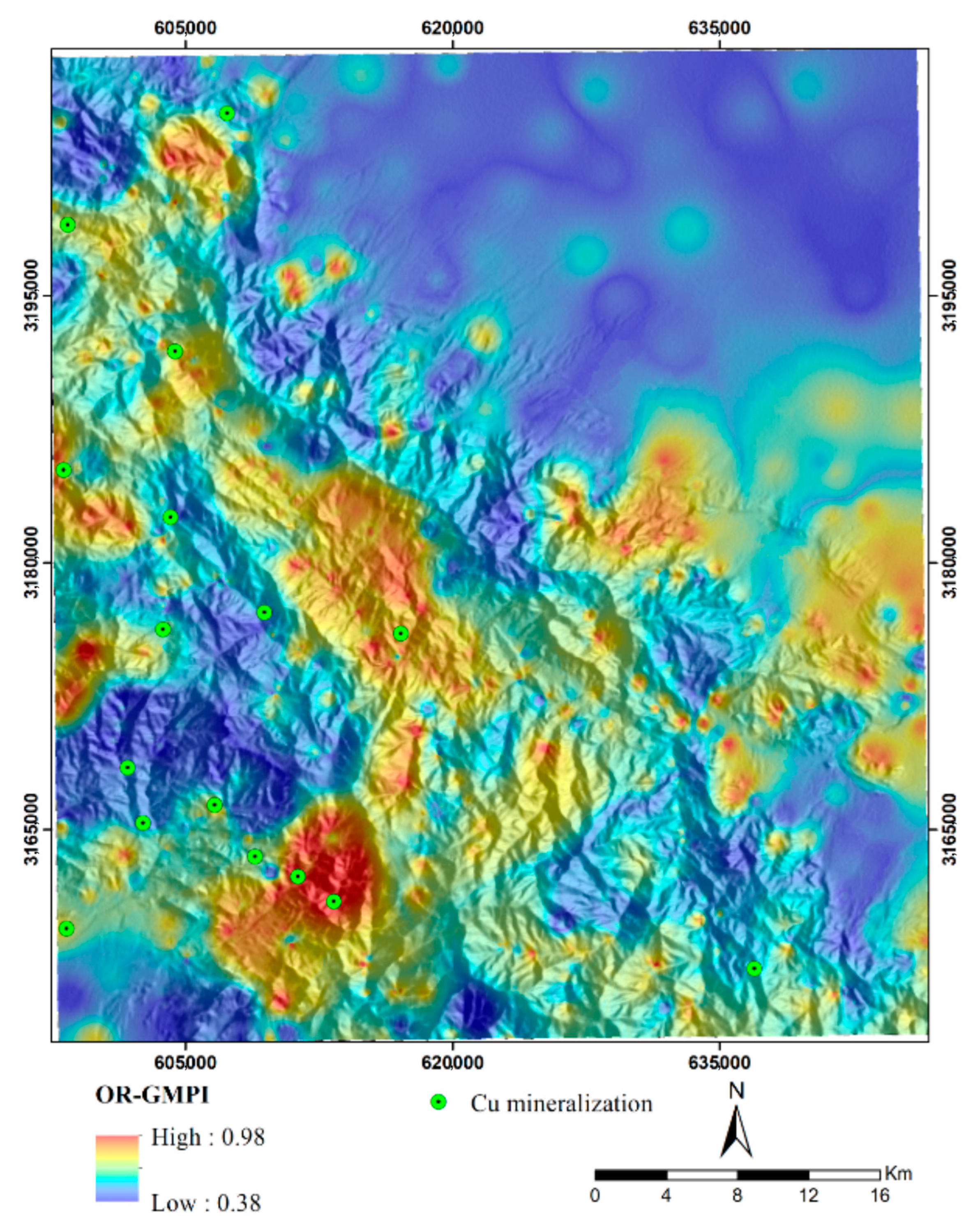
3.2. Geochemical Anomaly Evidence

One of the most significant layers in MPM is the evidence layer of multi-element geochemical anomalies [57,59,60]. The analysis of stream sediment geochemical data and the identification of anomalous samples is a widely used technique in regional-scale mineral exploration to locate mineral deposits [61,62,63,64]. In this research, data preparation and normalization were first performed to generate multi-element geochemical footprints. Then, a factor analysis (FA) [65], as a multivariate statistics method, was applied to the processing of the geochemical dataset, which includes the elements Au, Hg, Sb, As, Cu, Zn, Ag, and Pb. These elements were selected based on the conceptual model of the targeted mineral deposit type. According to this conceptual model (i.e., the mineral system of porphyry copper deposits) and previous studies, these elements were associated with such deposits and widely used for target generation [57,58,66,67]. The correlation matrix (Pearson) of these elements was calculated (

Table 2. Correlation matrix for 8 elements (Pearson).

Elements	Zn	Pb	Ag	Cu	As	Sb	Hg	Au
Zn	1	−0.126	−0.409	−0.020	−0.381	0.032	−0.181	0.430
Pb	−0.126	1	0.596	−0.595	−0.007	−0.412	−0.595	−0.144
Ag	−0.409	0.596	1	−0.500	0.229	−0.354	−0.375	−0.181
Cu	−0.020	−0.595	−0.500	1	−0.043	0.482	0.677	0.012
As	−0.381	−0.007	0.229	−0.043	1	0.533	−0.025	−0.292
Sb	0.032	−0.412	−0.354	0.482	0.533	1	0.351	−0.087
Hg	−0.181	−0.595	−0.375	0.677	−0.025	0.351	1	0.001
Au	0.430	−0.144	−0.181	0.012	−0.292	−0.087	0.001	1

). In the next step, FA was implemented. As shown in

Table 3. Implementation of FA on geochemical data.

Elements	Factor 1	Factor 2	Factor 3
Au	0.031	0.685	−0.186
Hg	0.872	−0.209	−0.036
Sb	0.437	0.081	0.829
As	−0.131	−0.363	0.861
Cu	0.872	−0.019	0.097
Ag	−0.654	−0.525	−0.076
Pb	−0.803	−0.207	−0.162
Zn	−0.034	0.906	−0.033

, all three derived factors (i.e., Factor 1, Factor 2, and Factor 3) are associated with copper mineralization in the Jebal Barez region and can be considered representative indicators of mineralization. Consequently, the results of all factors were utilized to construct the multi-element geochemical anomaly layer. To achieve this, the factor scores obtained from FA were transferred to fuzzy space using the logistic function of Equation (1). This function, known as the Geochemical Probability Index (GMPI) [58], is an appropriate method for fuzzy weighting and generating multi-element geochemical evidence layers. Several studies have demonstrated that utilizing the GMPI in MPM can enhance the prediction rates of the final prospectivity models [57,68,69,70].

$$GMPI={\displaystyle \frac{e^{Fs}}{1+e^{Fs}}}$$

(1)

After transferring the factor scores to the fuzzy space, the fuzzy OR operator was utilized to combine the results of the three GMPI maps. Subsequently, a geochemical map associated with mineralization was generated. As shown in Figure 3, there is a significant spatial correlation between the known mineral deposits, intrusive rocks, and the anomalies identified in the produced map.

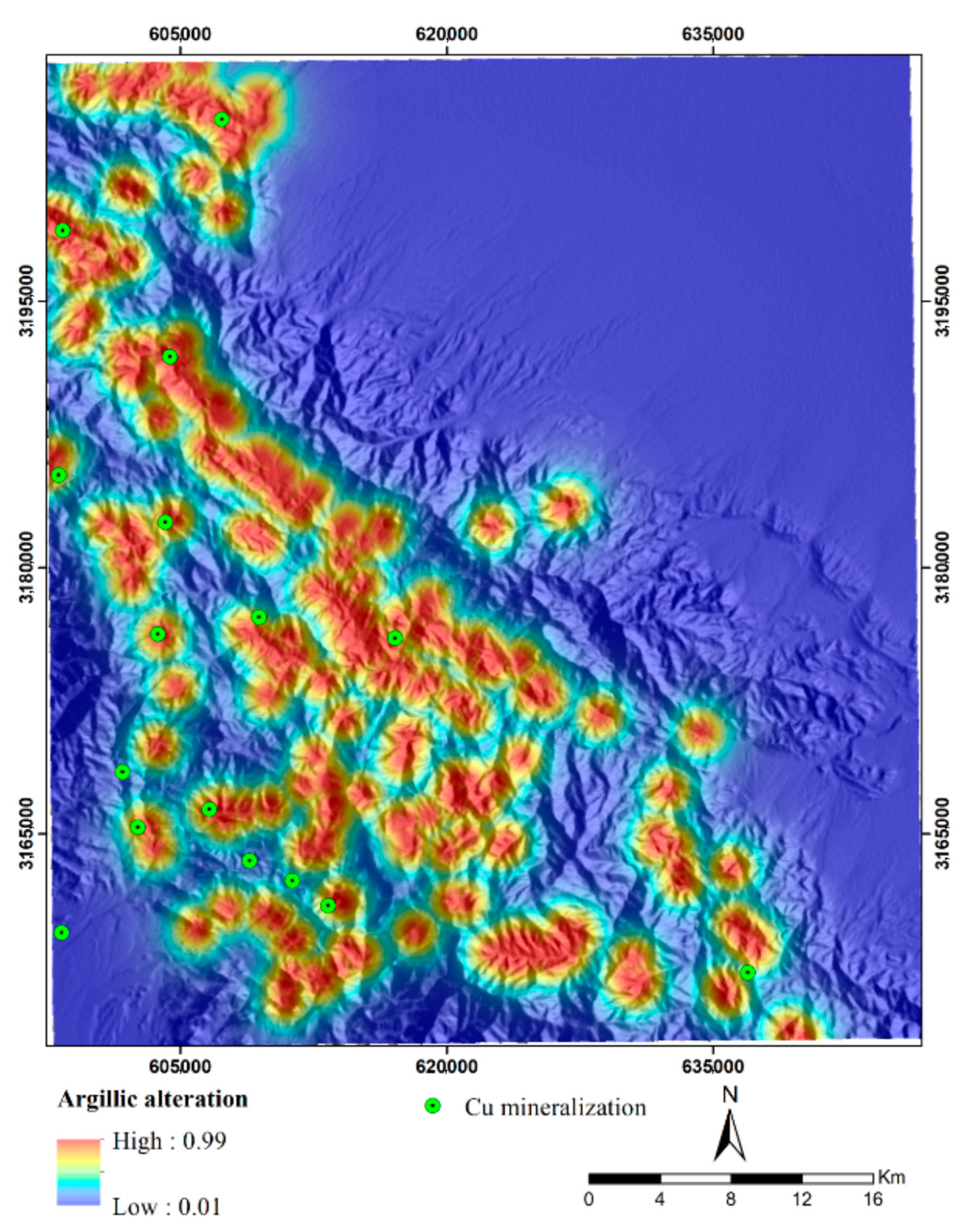
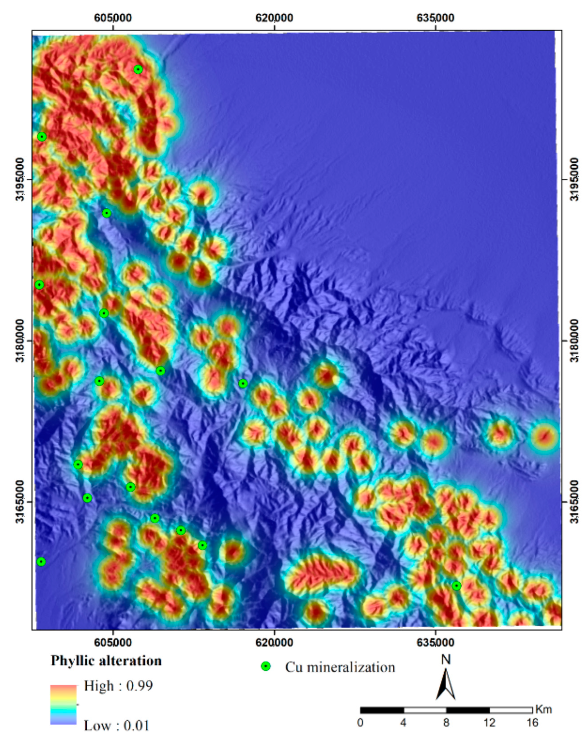
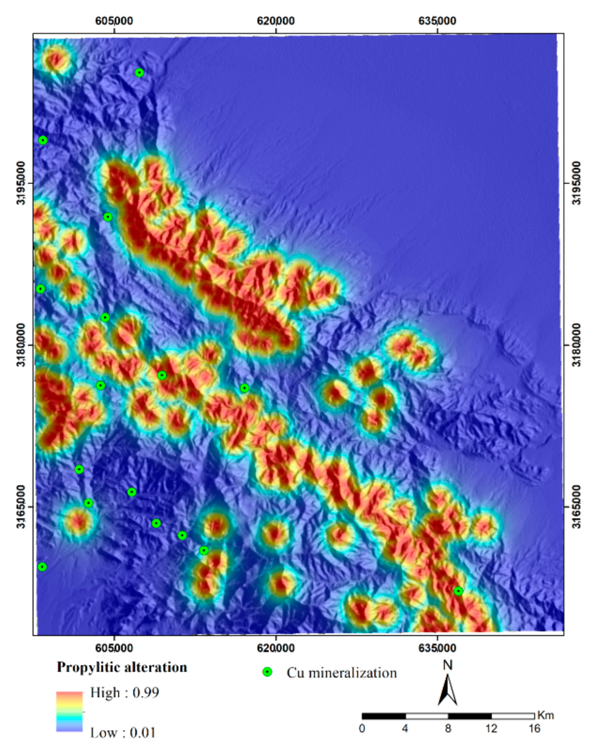
3.3. Distance-Based Generation of Evidence Layers for Hydrothermal Alterations

Hydrothermal fluids have an essential role in the formation of hydrothermal deposits, such as porphyry copper. The movement and migration of these fluids lead to significant changes in the chemical composition and mineralogy of the surrounding rocks related to mineralization. Hydrothermal alterations surrounding porphyry copper deposits typically exhibit specific patterns and often encompass a larger surface area compared to the mineralization. Therefore, identifying zones with hydrothermal alterations is a fundamental aspect of the exploration of porphyry copper deposits on a regional scale [71,72]. The spectral characteristics of indicator minerals within these zones facilitate their identification through satellite image processing. As a result, hydrothermal alteration data can be utilized to generate remote sensing evidence layers for the potential mineral modeling of porphyry copper deposits. In this study, hydrothermal alteration zones, including phyllic, argillic, propylitic, and iron oxide alterations, were identified through ASTER image processing using band ratios and spectral angle mapper techniques. Band ratios of 4/2, 5/6, 7/6, and 9/8 were used to map several alteration zones (i.e., iron oxide, argillic, phyllic, and propylitic) [71,72,73,74]. These ratios were selected based on the spectral features of the index minerals linked to each alteration and previous geological remote sensing studies. Also, the SAM method (along with the USGS library) was utilized to select endmember minerals (i.e., kaolinite, muscovite, and chlorite). The spectral absorption characteristics of these endmember minerals in the SWIR band of the ASTER image were applied as the spectral range to detect the alteration zones (i.e., argillic, phyllic, and propylitic). Subsequently, distance maps to these alteration zones were generated to create evidence layers. The values of these maps were then transformed to a 0-1 scale using the logistic function [75] defined in Equation (2) (Figure 4, Figure 5, Figure 6 and Figure 7). Notably, areas with higher values in these layers are predominantly associated with intrusive and igneous rocks, particularly within the faulted intrusive units located in the southern and southwestern parts of the region. This suggests that intrusive rocks and the intense activity of hydrothermal fluids in the Jebal Barez area have contributed to the development of extensive hydrothermal alteration zones.

$$F_E={\displaystyle \frac{1}{1+e^{-s\left(E-i\right)}}}$$

(2)

where $s$ denotes the slope of the logistic function, and $i$ is the inflection point of the logistic function. The values of $i$ and $s$ are derived from Equations (3) and (4), respectively.

$$i={\displaystyle \frac{E_{max}+E_{min}}{2}}$$

(3)

$$s={\displaystyle \frac{9.2}{E_{max}-E_{min}}}$$

(4)

3.4. Fault Density Evidence Layer

Various mineral deposits are correlated with specific geological structures, particularly faults and fractures [76]. Previous MPM studies have demonstrated the crucial role of faults in identifying prospective areas for intrusive-related deposits, such as porphyry copper mineralization [57,77]. These faults, along with fractured and crushed zones, act as suitable conduits for the movement of hydrothermal and ore-bearing magmatic fluids, promoting the development of alteration zones linked to mineralization. As a result, areas with a high fault density are considered favorable for porphyry copper exploration.

In this study, the faults from the Jebal Barez geological map (1:100,000 scale) were digitized. To create the fault density map, the total length of faults per pixel was calculated. Since the values of the fault density map were unbounded, a logistic function (Equation (2)) was utilized to transform these values into fuzzy space (Figure 8).

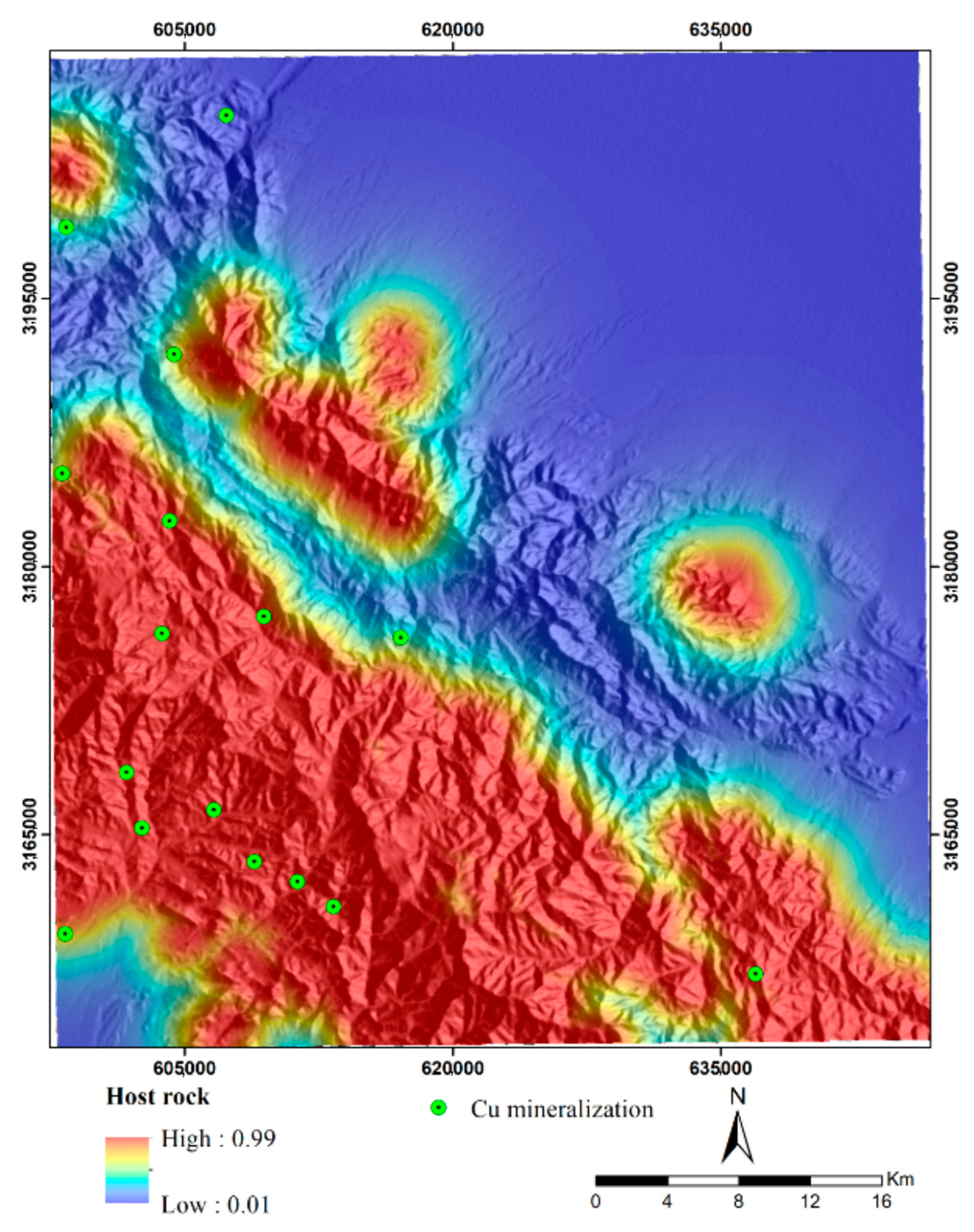
3.5. Host Rock Evidence Layer

Porphyry copper deposits within the UDMZ show a strong spatial and genetic relationship with various intrusive rocks, including granite, granodiorite, monzonite, and quartz monzonite [70,78,79]. These rocks serve as proxy indicators of magmatic-related processes that contribute to the formation of ore-forming materials. The likelihood of porphyry copper deposit formation is higher in proximity to these rocks. Therefore, regions near intrusive rocks are considered to have higher exploration potential than more distant regions [70]. The majority of porphyry copper deposits, particularly the classic mineralization types found in the UDMZ, such as Sarcheshmeh and Sungun, exhibit a close association with intrusive rocks. This correlation has been confirmed through geological studies and various MPM investigations [78,80]. Thus, this study generated a distance map from intrusive rocks as a key evidence layer for modeling porphyry copper mineral potentials. The Euclidean distance from intrusive rocks was calculated to generate this layer, and its values were transformed into fuzzy space using a logistic function (Equation (2)). As demonstrated in Figure 9, a significant number of known mineral deposits in the Jebal Barez region exhibit a strong spatial relationship with high values of this geological layer. Therefore, this layer is considered one of the most crucial layers in the prospectivity modeling of porphyry copper deposits.

4. Methodology

4.1. Predication-Area Plot

Evaluating the degree of importance and the prediction rates associated with the generated prospectivity models is essential in the MPM tasks. In this regard, the prediction-area (P-A) plot [81,82] can be utilized. This plot is based on ground truth positive samples (known as mineral deposits) and is considered one of the most effective data-driven methods for the quantitative evaluation of prospectivity models. The accuracy of mineral potential models can be evaluated by analyzing the spatial relationship between the known mineral deposits and each of the generated model classes. This plot consists of two curves [82,83,84], and their intersection point indicates the prediction rate and accuracy of the prospectivity model. If the intersection point of a specific prospectivity model indicates a higher prediction rate (left axis) compared to the plots of other models, it implies that the former model has successfully identified a greater number of known mineral deposits within a smaller area (right axis). The normalized density of the MPM model, as a numerical assessment index, is derived based on the intersection of the prediction rate and occupied area curves. This index is obtained by calculating the ratio of the prediction rate to the occupied area at the intersection point (Equation (5)). Finally, the weight of each prospectivity model is determined based on Equation (6).

$$N_d={\displaystyle \frac{P_r}{O_a}}$$

(5)

$$w_E=Ln{N}_d$$

(6)

where $N_d$ refers to the normalized density, and $P_r$ and $O_a$ are the prediction rate and occupied area, respectively, obtained from the intersection point of the P-A plot.

This index can indicate the accuracy of the constructed model by utilizing ground truth labels. Considering the influence of various hyperparameters on the accuracy of machine learning algorithms, they can be used to determine the model’s accuracy and evaluate the impact of different hyperparameters on the mineral prospectivity models produced. Ultimately, the best model can be selected based on the highest weight. Figure 10 demonstrates the methodology flowchart of this study.

4.2. Isolation Forest

The isolation forest (IF) algorithm depends on two key parameters: the number of isolation trees (t) and the maximum number of features (m). To train the model, one isolation tree (ITree) is constructed as follows [43,85]:

A random sample $D_i$ is selected from the dataset $D$, which contains $n$ instances with $m$ features.

A feature ($A$) is selected from the randomly chosen subset of features $\left(m\right)$, and a cut-point $P_a$ is randomly determined within its range.

The sample $D_i$ is divided into two sub-samples by splitting at the cut-point $P_a$, forming left and right subtrees.

The process continues until each instance is isolated or the tree reaches a predetermined height.

To form the IF, $t$ ITrees are generated. In the IF, the anomalous instances are identified by calculating the expected depth of ITrees for given N training instances (Equation (7)) for each instance, where anomalies typically have shorter path lengths in the trees. The expected depth for a data point $X$ and n instances is computed using Equation (7), where $H\left(n\right)=\ln n+\gamma$ and $\gamma$ is the Euler constant.

$$c\left(n\right)=2H\left(n-1\right)-\left({\displaystyle \frac{2\left(n-1\right)}{n}}\right)$$

(7)

The formula for determining the detailed anomaly score is given by the following:

$$s\left(X, n\right)=2^{-{\displaystyle \frac{E\left(h\left(X\right)\right)}{c\left(n\right)}}}$$

(8)

where $h\left(X\right)$ is the depth of the instance $X$ in the particular ITree, and $E\left(h\left(X\right)\right)$ is its average over all ITrees. Since anomalies are isolated more quickly, they have shorter path lengths, resulting in a score closer to 1.

4.3. Extended Isolation Forest

In the original IF algorithm, nodes are split along the vertical or horizontal axes. This approach introduces a bias because the split occurs only along the axes, which limits the flexibility of the model and can distort the anomaly score map. The extended isolation forest (EIF) [86] was developed to address this limitation by allowing splits in any direction, not just vertical or horizontal ones. While the scoring phase remains unchanged from IF, the training phase undergoes a significant modification. Instead of splitting nodes strictly along the axes, EIF selects both a random point and a random direction by considering a combination of all dimensions. This adjustment eliminates the bias introduced by the axis-parallel cuts in the original IF.

This adjustment in EIF corrects the biases inherent in the original IF, leading to more accurate anomaly detection. By splitting nodes along random directions, EIF creates more evenly distributed splits, which reduces the risk of generating biased anomaly scores. This results in more consistent anomaly scores and improves the overall reliability of the model, especially in complex datasets. Their comparative study highlights that EIF anomaly maps are more evenly distributed, which helps in better detecting anomalies without introducing the bias associated with axis-based divisions [47,86].

The EIF implementation has two key hyperparameters to configure, namely, the “extension level” and the number of ITrees. The extension level is in the range of $\left[0, P-1\right]$, where $P$ is the number of features in the dataset. A value of 0 corresponds to the original IF, where splits are axis-parallel cuts. As the extension level increases toward $P-1$, allowing for splits at various angles, the IF’s bias is reduced.

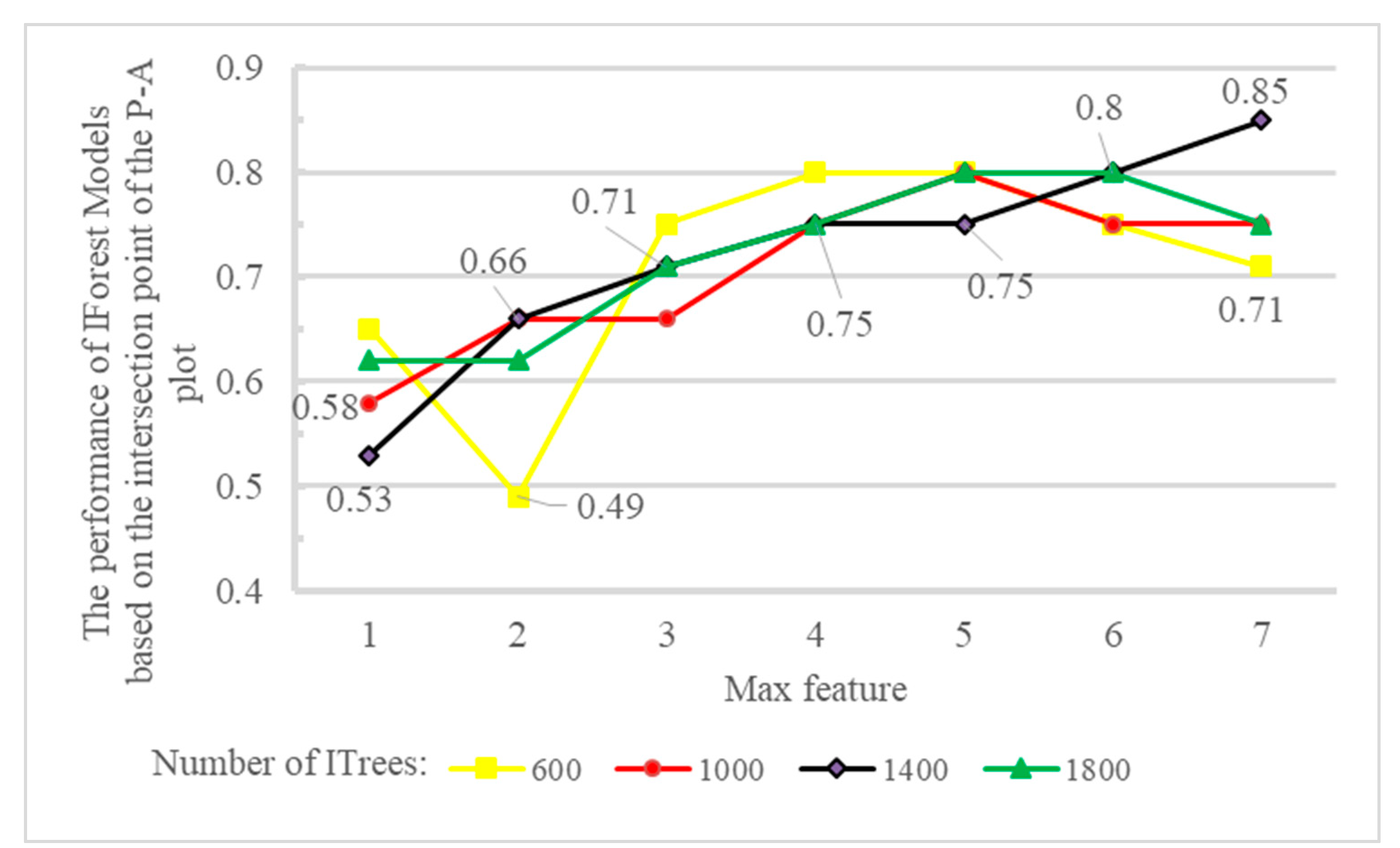
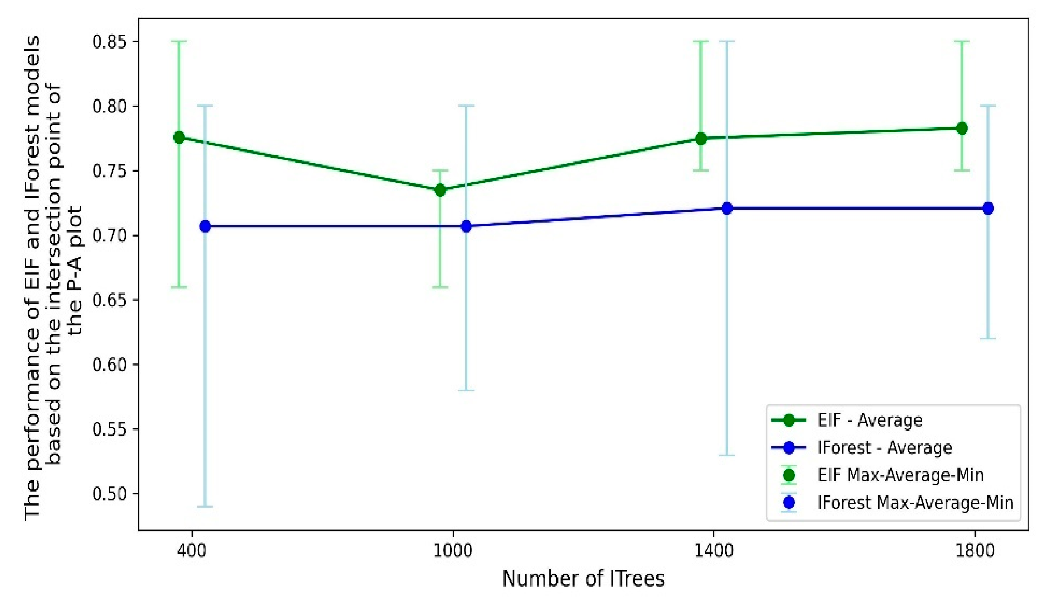
5. Algorithm Results

After constructing the evidence layers, the IF and EIF were employed for data integration, with a consideration to optimize the key hyperparameters. For the IF algorithm, two key hyperparameters, namely, the “number of ITrees” and “maximum features” were optimized to maximize the performance of the prospectivity model. The maximum features were adjusted from 1 to 7 (the maximum number of evidence layers), while the number of ITrees was set to 600, 100, 1400, and 1800 (

Table 4. Important hyperparameters of IF and EIF and their corresponding values.

Algorithm	Hyperparameter	Values	Total
IF	Number of ITrees	[600, 1000, 1400, 1800]	28
	Max features	[1, 2, 3, 4, 5, 6, 7]
EIF	Number of ITrees	[600, 1000, 1400, 1800]	24
	Extension level	[1, 2, 3, 4, 5, 6]

). For the EIF, the same number of ITrees was used, while the “Extension level” ranged from one to six (the number of evidence layers minus one) (Table 4).

In total, 28 distinct models were generated using the IF algorithm, and each was evaluated based on the P-A plot. First, the 28 generated models were classified using the “natural break” method, and P-A plots were plotted using the thresholds derived from this method. Subsequently, the weight of each model was computed, which uses the intersection point of the prediction rate and curves. Figure 11 illustrates the impact of different values for the maximum features and number of ITrees on the weight obtained for each IF model. As can be observed, increasing the maximum features generally improves the performance of the IF model, regardless of the number of ITrees used. For lower values of the maximum features (1 and 2), the models exhibited lower performance, with scores ranging between 0.49 and 0.66. This pattern contrasts with higher values of maximum features (4 to 7), where the performance significantly improved and reached values between 0.71 and 0.85. For instance, models built with 1400 ITrees show a noticeable improvement in performance as the maximum feature values increase. Specifically, as the maximum feature values increased, the model’s performance improved gradually, from 0.53 (maximum features set to 1) to 0.85 (maximum features set to 7). This indicates that the model’s ability to capture important patterns improves with higher values for the maximum features.

Across all of the 28 IF models generated, the model with a maximum feature value of 7 and 1400 ITrees has the highest performance, with a weight of 0.85. Consequently, this configuration was selected as the optimal hyperparameter value for IF MPM in the study. Figure 12 illustrates the performance of various EIF models based on the extension level and the number of ITrees. The performance of EIF models does not follow a consistent pattern when the extension is increased, and the performance patterns show a mixed relationship between the extension level and the number of ITrees.

The performance of the EIF models fluctuates across the different extension levels, which indicates that a higher extension level does not necessarily lead to better results (Figure 12). For example, while the EIF model with 1400 ITrees shows its highest performance at the lowest extension level of 1, the performance decreases across the subsequent levels and never reaches that initial peak again. However, the EIF model with 600 ITrees peaks at the extension levels of 1 and 3. This pattern contrasts with the IF models, where the performance increases more predictably with higher max features (Figure 11). The fluctuation in the performance of the EIF models may be due to added complexity introduced by higher extension levels, which can make it harder for the model to isolate anomalies effectively. This result suggests that, while both models rely on key hyperparameters to optimize performance, the relationship between these hyperparameters and the model output is more straightforward and predictable in the IF models, whereas EIF models require more careful tuning to avoid performance drops across the different extension levels. Figure 13 and Figure 14, respectively, depict the P-A plots and the corresponding prospectivity models generated by the optimal configurations of IF and EIF. Figure 13a and Figure 14a, respectively, depict the P-A plot and the corresponding prospectivity model generated by the max feature value of 7 and 1400 ITrees for IF. Figure 13b and Figure 14b, respectively, depict the P-A plot and the corresponding prospectivity model generated by the extension level value of 1 and 600 ITrees for EIF.

The prospectivity models generated by IF (Figure 14a) and EIF (Figure 14b) generally show similar patterns, but the EIF intensifies the high-value regions more distinctly. In the EIF model (see Figure 14b), the high-potential areas (red) are more concentrated and have sharper boundaries, which makes anomalous areas more distinct. In contrast, the IF model (Figure 14a) shows a more gradual transition, with smoother and less intense delineation of high-potential areas, resulting in a less distinct identification of anomalies.

The comparison of the prospectivity models generated by the two unsupervised tree-based algorithms, IF and EIF (Figure 14), with the geological map of the study area (Figure 1) indicated that the anomalous zones identified by both methods are consistent with the andesitic units, tuffs, rhyolites, pyroclastic units, and intrusive rocks. Furthermore, these methods have suitably predicted many of the known mineral deposits in the region. Therefore, it can be inferred that both algorithms demonstrate a high level of effectiveness in identifying exploration targets associated with mineralization in the study area.

In Figure 11 and Figure 12, we investigate the impact of key hyperparameters on the performance of the IF and EIF models. As illustrated in Figure 15, our comparative analysis specifically focuses on the average results across different numbers of ITrees and assesses the impact of this hyperparameter for both algorithms. The results indicate that the average performance remains relatively stable as the number of ITrees increases. This pattern is consistent for both the IF and EIF models and suggests that the average performance remains stable regardless of the number of ITrees when averaged over multiple runs with different values for the other hyperparameter (i.e., max feature for IF and extension level for EIF). This stability indicates that increasing the number of ITrees may not contribute substantially to enhancing the models’ anomaly detection capabilities. These patterns also can be observed in Figure 11 and Figure 12, as the models with a higher number of ITrees do not necessarily have higher performance. This indicates that both models reach a point where adding more trees does not contribute to better accuracy, particularly when considering averaged results.

As shown in Figure 15, the EIF model consistently outperforms the IF model in terms of average performance across all tested ITree values, and the average performance of EIF is always higher than that of the IF model, showing its enhanced capability for more reliable anomaly detection. Furthermore, the range of performance for the EIF model is considerably smaller compared to the IF model, indicating that EIF is less affected by changes in other hyperparameter values, i.e., extension level. In contrast, the IF model shows a wider range of performance, indicating higher sensitivity to max feature hyperparameters and potential instability under certain hyperparameter configurations. This stability in the EIF model could be attributed to its unique mechanism of isolating anomalies using extended, multi-dimensional hyperplanes. Therefore, the comparative study demonstrates the superiority of the EIF model in terms of performance across varying hyperparameter settings. In this study, to identify prospecting zones linked to the porphyry copper mineralization and generate binary prospectivity models (Figure 16 and Figure 17), a percentile of 90% was used. A percentile of 90% for the IF and EIF prospectivity models was obtained at 0.68 and 0.69, respectively.

6. Discussion

In MPM studies, evidence layers are created based on the conceptual model of the sought mineralization and known mineral deposits in the study area. This leads to high values in each evidence layer typically having a strong spatial correlation with known deposits. Therefore, in exploratory datasets, other samples with high values can be associated with the target mineralization and identified as prospective areas [13,17]. As a result, unsupervised machine learning algorithms, such as the IF, which identifies samples with high (anomalous) values, can be employed to generate mineral potential maps.

The IF and EIF algorithms are based on the assumption that datasets contain a limited number of anomalous samples whose values are significantly different from the background. These algorithms directly identify and isolate anomalous samples within the dataset. Due to their smaller numbers and different values for some features, anomalous samples are more easily isolated in ITrees compared to normal or background samples. Generally, they traverse shorter paths in each ITree compared to normal samples. The IF algorithm relies on randomness in selecting features (evidence layers) and thresholds within those features [46]. Thus, the “max features” hyperparameter, which determines the number of features to use during the construction of each ITree, can significantly affect the final model. As demonstrated by the results of this study, the performance of the mineral potential model is highly sensitive to this hyperparameter. Specifically, increasing the number of features generally improves the model’s performance (Figure 8). This suggests that incorporating all the evidence layers produced in this study can enhance the final model’s effectiveness. In other words, setting the max features hyperparameter to 7 (equal to the number of evidence layers) allows the IF algorithm to simultaneously consider all evidence layers and their relationships for identifying anomalous regions, ultimately improving the model’s ability to detect high-potential areas. Conversely, when smaller values (1 to 3) are assigned to this hyperparameter, only a few layers are used to identify anomalies, resulting in reduced model performance. However, based on the performance of the EIF model with different hyperparameter values (Figure 12), it is difficult to make a general conclusion about the impact of its hyperparameters on the final model’s performance.

As discussed by [17] and [13], MPM can be fundamentally considered as an anomaly detection task, where target mineralization represents deviations from the background of the geodataset. This conceptual alignment makes IF and its variants (e.g., EIF) particularly suitable for MPM, as their core objective is identifying anomalous samples from the background. While these methods offer practical advantages, such as a few hyperparameters and low computational costs, our analysis demonstrates that careful hyperparameter optimization remains critical for the best performance in a real context. Additionally, as highlighted by [87], IF exhibits consistent performance across varying dimensions, particularly in a high dimension. This contrasts with methods like LOF, which are sensitive to dimensionality. IF’s robustness against high-dimensional geodatasets reduces concerns about dataset dimensionality, which is a significant advantage over other methods, such as LOF. However, to validate our results and ensure applicability in greenfield explorations, more studies should test the proposed framework across diverse regions with varying geological complexity and geochemical signatures.

7. Conclusions

Mineral prospectivity mapping (MPM) can be regarded as an anomaly detection process within the field of mineral exploration and exploration information system (EIS) frameworks, as mineralization is a relatively rare and spatially irregular geological phenomenon in the Earth’s crust. In this context, unsupervised anomaly detection (UAD) algorithms based on machine learning are effective in identifying complex, non-linear patterns associated with high-potential mineralized zones. Moreover, they facilitate the extraction of exploration patterns from evidence layers, which are developed in alignment with the conceptual model of the mineral deposit type sought. This study highlights the performance of tree-based anomaly detection algorithms, namely, IF and EIF, in detecting irregular and subtle patterns associated with porphyry copper deposits. The results demonstrated that both algorithms provide effective support for unsupervised exploration targeting. The anomalous zones identified by these methods are spatially correlated with geological features, including andesites, tuffs, rhyolites, pyroclastics, and intrusive rocks. Furthermore, a quantitative analysis using the prediction-area plot showed that IF and EIF exhibit strong performance in terms of prediction rate. Additionally, the results emphasize the significant impact of hyperparameter tuning in enhancing the accuracy of generated prospectivity models. IF demonstrated a more transparent and structured framework for hyperparameter optimization, while EIF lacked this level of clarity, making the optimization process more challenging.

References

1. Yousefi, M.; Carranza, E.J.M. Geometric average of spatial evidence data layers: A GIS-based multi-criteria decision-making approach to mineral prospectivity mapping. Comput. Geosci. 2015, 83, 72–79. [Google Scholar] [CrossRef]
2. Yin, B.; Zuo, R.; Sun, S. Mineral prospectivity mapping using deep self-attention model. Nat. Resour. Res. 2023, 32, 37–56. [Google Scholar] [CrossRef]
3. Bahrami, Y.; Hasani, H.; Maghsoudi, A. Application of AHP-TOPSIS method to model copper mineral potencial in the Abhar 1:100000 geological map, NW Iran. Res. Earth Sci. 2021, 12, 41–57. [Google Scholar] [CrossRef]
4. Aali, A.A.; Shirazy, A.; Shirazi, A.; Pour, A.B.; Hezarkhani, A.; Maghsoudi, A.; Hashim, M.; Khakmardan, S. Fusion of remote sensing, magnetometric, and geological data to identify polymetallic mineral potential zones in Chakchak Region, Yazd, Iran. Remote Sens. 2022, 14, 6018. [Google Scholar] [CrossRef]
5. Shirazi, A.; Hezarkhani, A.; Beiranvand Pour, A.; Shirazy, A.; Hashim, M. Neuro-Fuzzy-AHP (NFAHP) technique for copper exploration using Advanced Spaceborne Thermal Emission and Reflection Radiometer (ASTER) and geological datasets in the Sahlabad mining area, east Iran. Remote Sens. 2022, 14, 5562. [Google Scholar] [CrossRef]
6. Bonham-Carter, G. Geographic Information Systems for Geoscientists: Modelling with GIS; Elsevier: Amsterdam, The Netherlands, 1994. [Google Scholar]
7. Hoseinzade, Z.; Shojaei, M.; Khademi, F.; Mokhtari, A.R.; Saremi, M. Integration of deep learning models for mineral prospectivity mapping: A novel Bayesian index approach to reducing uncertainty in exploration. Model. Earth Syst. Environ. 2025, 11, 161. [Google Scholar] [CrossRef]
8. Yousefi, M.; Carranza, E.J.M.; Kreuzer, O.P.; Nykänen, V.; Hronsky, J.M.; Mihalasky, M.J. Data analysis methods for prospectivity modelling as applied to mineral exploration targeting: State-of-the-art and outlook. J. Geochem. Explor. 2021, 229, 106839. [Google Scholar] [CrossRef]
9. Carranza, E.J.M. Geochemical Anomaly and Mineral Prospectivity Mapping in GIS; Elsevier: Amsterdam, The Netherlands, 2008. [Google Scholar]
10. Yousefi, M.; Nykänen, V.; Harris, J.; Hronsky, J.M.; Kreuzer, O.P.; Bertrand, G.; Lindsay, M. Overcoming survival bias in targeting mineral deposits of the future: Towards null and negative tests of the exploration search space, accounting for lack of visibility. Ore Geol. Rev. 2024, 172, 106214. [Google Scholar] [CrossRef]
11. Abedi, M.; Kashani, S.B.M.; Norouzi, G.-H.; Yousefi, M. A deposit scale mineral prospectivity analysis: A comparison of various knowledge-driven approaches for porphyry copper targeting in Seridune, Iran. J. Afr. Earth Sci. 2017, 128, 127–146. [Google Scholar] [CrossRef]
12. Yousefi, M.; Lindsay, M.D.; Kreuzer, O. Mitigating uncertainties in mineral exploration targeting: Majority voting and confidence index approaches in the context of an exploration information system (EIS). Ore Geol. Rev. 2024, 165, 105930. [Google Scholar] [CrossRef]
13. Mirzabozorg, S.A.A.S.; Abedi, M. Recognition of mineralization-related anomaly patterns through an autoencoder neural network for mineral exploration targeting. Appl. Geochem. 2023, 158, 105807. [Google Scholar] [CrossRef]
14. Saremi, M.; Bagheri Ghadikolaei, S.M.; Agha Seyyed Mirzabozorg, S.A.; Hassan, N.E.; Hoseinzade, Z.; Maghsoudi, A.; Rezania, S.; Ranjbar, H.; Zoheir, B.; Beiranvand Pour, A. Evaluation of Deep Isolation Forest (DIF) Algorithm for Mineral Prospectivity Mapping of Polymetallic Deposits. Minerals 2024, 14, 1015. [Google Scholar] [CrossRef]
15. Abedi, M.; Norouzi, G.-H. Integration of various geophysical data with geological and geochemical data to determine additional drilling for copper exploration. J. Appl. Geophys. 2012, 83, 35–45. [Google Scholar] [CrossRef]
16. Qaderi, S.; Maghsoudi, A.; Pour, A.B.; Rajabi, A.; Yousefi, M. DCGAN-Based Feature Augmentation: A Novel Approach for Efficient Mineralization Prediction Through Data Generation. Minerals 2025, 15, 71. [Google Scholar] [CrossRef]
17. Yousefi, M.; Kreuzer, O.P.; Nykänen, V.; Hronsky, J.M. Exploration information systems–A proposal for the future use of GIS in mineral exploration targeting. Ore Geol. Rev. 2019, 111, 103005. [Google Scholar] [CrossRef]
18. Yousefi, M.; Carranza, E.J.M. Data-driven index overlay and Boolean logic mineral prospectivity modeling in greenfields exploration. Nat. Resour. Res. 2016, 25, 3–18. [Google Scholar] [CrossRef]
19. Rezapour, M.J.; Abedi, M.; Bahroudi, A.; Rahimi, H. A clustering approach for mineral potential mapping: A deposit-scale porphyry copper exploration targeting. Geopersia 2020, 10, 149–163. [Google Scholar]
20. Xiong, Y.; Zuo, R.; Carranza, E.J.M. Mapping mineral prospectivity through big data analytics and a deep learning algorithm. Ore Geol. Rev. 2018, 102, 811–817. [Google Scholar] [CrossRef]
21. Chen, G.; Huang, N.; Wu, G.; Luo, L.; Wang, D.; Cheng, Q. Mineral prospectivity mapping based on wavelet neural network and Monte Carlo simulations in the Nanling W-Sn metallogenic province. Ore Geol. Rev. 2022, 143, 104765. [Google Scholar] [CrossRef]
22. Li, S.; Chen, J.; Liu, C. Overview on the development of intelligent methods for mineral resource prediction under the background of geological big data. Minerals 2022, 12, 616. [Google Scholar] [CrossRef]
23. Lou, Y.; Liu, Y. Mineral prospectivity mapping of tungsten polymetallic deposits using machine learning algorithms and comparison of their performance in the Gannan region, China. Earth Space Sci. 2023, 10, e2022EA002596. [Google Scholar] [CrossRef]
24. Abedi, M.; Norouzi, G.-H.; Bahroudi, A. Support vector machine for multi-classification of mineral prospectivity areas. Comput. Geosci. 2012, 46, 272–283. [Google Scholar] [CrossRef]
25. Shirazi, A.; Shirazy, A.; Hezarkhani, A. An Artificial Intelligence (AI)-Based Model for Optimal Exploratory Surveys; GRIN Verlag: Munich, Germany, 2024. [Google Scholar]
26. Zuo, R.; Carranza, E.J.M. Support vector machine: A tool for mapping mineral prospectivity. Comput. Geosci. 2011, 37, 1967–1975. [Google Scholar] [CrossRef]
27. Zhang, S.; Carranza, E.J.M.; Xiao, K.; Wei, H.; Yang, F.; Chen, Z.; Li, N.; Xiang, J. Mineral prospectivity mapping based on isolation forest and random forest: Implication for the existence of spatial signature of mineralization in outliers. Nat. Resour. Res. 2022, 31, 1981–1999. [Google Scholar] [CrossRef]
28. Zhang, S.; Xiao, K.; Carranza, E.J.M.; Yang, F. Maximum entropy and random forest modeling of mineral potential: Analysis of gold prospectivity in the Hezuo–Meiwu district, west Qinling Orogen, China. Nat. Resour. Res. 2019, 28, 645–664. [Google Scholar] [CrossRef]
29. Qaderi, S.; Maghsoudi, A.; Pour, A.B.; Yousefi, M. Geological Controlling Factors on Mississippi Valley-Type Pb-Zn Mineralization in Western Semnan, Iran. Minerals 2024, 14, 957. [Google Scholar] [CrossRef]
30. Carranza, E.j.m.; Hale, M. Logistic regression for geologically constrained mapping of gold potential, Baguio district, Philippines. Explor. Min. Geol. 2001, 10, 165–175. [Google Scholar] [CrossRef]
31. Rahimi, H.; Abedi, M.; Yousefi, M.; Bahroudi, A.; Elyasi, G.-R. Supervised mineral exploration targeting and the challenges with the selection of deposit and non-deposit sites thereof. Appl. Geochem. 2021, 128, 104940. [Google Scholar] [CrossRef]
32. Rodriguez-Galiano, V.; Sanchez-Castillo, M.; Chica-Olmo, M.; Chica-Rivas, M. Machine learning predictive models for mineral prospectivity: An evaluation of neural networks, random forest, regression trees and support vector machines. Ore Geol. Rev. 2015, 71, 804–818. [Google Scholar] [CrossRef]
33. Li, S.; Chen, J.; Liu, C.; Wang, Y. Mineral prospectivity prediction via convolutional neural networks based on geological big data. J. Earth Sci. 2021, 32, 327–347. [Google Scholar] [CrossRef]
34. Li, S.; Chen, J.; Xiang, J. Applications of deep convolutional neural networks in prospecting prediction based on two-dimensional geological big data. Neural Comput. Appl. 2020, 32, 2037–2053. [Google Scholar] [CrossRef]
35. Mirzabozorg, S.A.A.S.; Abedi, M.; Yousefi, M. Enhancing training performance of convolutional neural network algorithm through an autoencoder-based unsupervised labeling framework for mineral exploration targeting. Geochemistry 2024, 84, 126197. [Google Scholar] [CrossRef]
36. Zhang, S.; Carranza, E.J.M.; Wei, H.; Xiao, K.; Yang, F.; Xiang, J.; Zhang, S.; Xu, Y. Data-driven mineral prospectivity mapping by joint application of unsupervised convolutional auto-encoder network and supervised convolutional neural network. Nat. Resour. Res. 2021, 30, 1011–1031. [Google Scholar] [CrossRef]
37. Zuo, R.; Wang, Z. Effects of random negative training samples on mineral prospectivity mapping. Nat. Resour. Res. 2020, 29, 3443–3455. [Google Scholar] [CrossRef]
38. Cheng, Q. Mapping singularities with stream sediment geochemical data for prediction of undiscovered mineral deposits in Gejiu, Yunnan Province, China. Ore Geol. Rev. 2007, 32, 314–324. [Google Scholar] [CrossRef]
39. Chen, Y. Mineral potential mapping with a restricted Boltzmann machine. Ore Geol. Rev. 2015, 71, 749–760. [Google Scholar] [CrossRef]
40. Chen, Y.; Wu, W. Isolation forest as an alternative data-driven mineral prospectivity mapping method with a higher data-processing efficiency. Nat. Resour. Res. 2019, 28, 31–46. [Google Scholar] [CrossRef]
41. Shahrestani, S.; Conoscenti, C.; Carranza, E.J.M. Assessment of LUNAR, iForest, LOF, and LSCP methodologies in delineating geochemical anomalies for mineral exploration. J. Geochem. Explor. 2025, 273, 107737. [Google Scholar] [CrossRef]
42. Chen, Y.; Wu, W. Application of one-class support vector machine to quickly identify multivariate anomalies from geochemical exploration data. Geochem. Explor. Environ. Anal. 2017, 17, 231–238. [Google Scholar] [CrossRef]
43. Liu, F.T.; Ting, K.M.; Zhou, Z.-H. Isolation forest. In Proceedings of the 2008 Eighth IEEE International Conference on Data Mining, Pisa, Italy, 15–19 December 2008; IEEE: Piscataway, NJ, USA, 2008. [Google Scholar]
44. Liu, F.T.; Ting, K.M.; Zhou, Z.-H. Isolation-based anomaly detection. ACM Trans. Knowl. Discov. Data (TKDD) 2012, 6, 1–39. [Google Scholar] [CrossRef]
45. Fadul, A.M.A. Anomaly Detection Based on Isolation Forest and Local Outlier Factor. Master’s Thesis, Africa University, Mutare, Africa, 2023. [Google Scholar]
46. Zheng, C.; Zhao, Q.; Fan, G.; Zhao, K.; Piao, T. Comparative study on isolation forest, extended isolation forest and generalized isolation forest in detection of multivariate geochemical anomalies. Glob. Geol. 2023, 26, 167–176. [Google Scholar]
47. Chabchoub, Y.; Togbe, M.U.; Boly, A.; Chiky, R. An in-depth study and improvement of Isolation Forest. IEEE Access 2022, 10, 10219–10237. [Google Scholar] [CrossRef]
48. Asadi, S.; Moore, F.; Zarasvandi, A. Discriminating productive and barren porphyry copper deposits in the southeastern part of the central Iranian volcano-plutonic belt, Kerman region, Iran: A review. Earth-Sci. Rev. 2014, 138, 25–46. [Google Scholar] [CrossRef]
49. Sadigh, S.; Mirmohammadi, M.; Asghari, O.; Porwal, A. Spatial distribution of porphyry copper deposits in Kerman Belt, Iran. Ore Geol. Rev. 2023, 153, 105251. [Google Scholar] [CrossRef]
50. Hezarkhani, A.; Williams-Jones, A.E. Controls of alteration and mineralization in the Sungun porphyry copper deposit, Iran; evidence from fluid inclusions and stable isotopes. Econ. Geol. 1998, 93, 651–670. [Google Scholar] [CrossRef]
51. Honarmand, M.; Ranjbar, H.; Shahabpour, J. Application of principal component analysis and spectral angle mapper in the mapping of hydrothermal alteration in the Jebal–Barez Area, Southeastern Iran. Resour. Geol. 2012, 62, 119–139. [Google Scholar] [CrossRef]
52. Fakhari, S.; Afzal, P.; Lotfi, M. Delineation of hydrothermal alteration zones for porphyry systems utilizing ASTER data in Jebal-Barez area, SE Iran. Iran. J. Earth Sci. 2019, 11, 80–92. [Google Scholar]
53. Pour, A.B.; Hashim, M. The application of ASTER remote sensing data to porphyry copper and epithermal gold deposits. Ore Geol. Rev. 2012, 44, 1–9. [Google Scholar] [CrossRef]
54. Hajaj, S.; El Harti, A.; Jellouli, A.; Pour, A.B.; Himyari, S.M.; Hamzaoui, A.; Hashim, M. ASTER data processing and fusion for alteration minerals and silicification detection: Implications for cupriferous mineralization exploration in the western Anti-Atlas, Morocco. Artif. Intell. Geosci. 2024, 5, 100077. [Google Scholar] [CrossRef]
55. Shirazi, A.; Shirazy, A.; Karami, J. Remote sensing to identify copper alterations and promising regions, Sarbishe, South Khorasan, Iran. Int. J. Geol. Earth Sci. 2018, 4, 36–52. [Google Scholar]
56. Shirazi, A.; Hezarkhani, A.; Shirazy, A.; Shahrood, I. Remote sensing studies for mapping of iron oxide regions, South of Kerman, Iran. Int. J. Sci. Eng. Appl. 2018, 7, 45–51. [Google Scholar] [CrossRef]
57. Saremi, M.; Yousefi, S.; Yousefi, M. Combination of Geochemical and Structural Data to Determine Exploration Target of Copper Hydrothermal Deposits in Feizabad District. J. Min. Environ. 2024, 15, 1089–1101. [Google Scholar]
58. Yousefi, M.; Kamkar-Rouhani, A.; Carranza, E.J.M. Geochemical mineralization probability index (GMPI): A new approach to generate enhanced stream sediment geochemical evidential map for increasing probability of success in mineral potential mapping. J. Geochem. Explor. 2012, 115, 24–35. [Google Scholar] [CrossRef]
59. Parsa, M.; Maghsoudi, A.; Yousefi, M.; Sadeghi, M. Recognition of significant multi-element geochemical signatures of porphyry Cu deposits in Noghdouz area, NW Iran. J. Geochem. Explor. 2016, 165, 111–124. [Google Scholar] [CrossRef]
60. Yousefi, M.; Kamkar-Rouhani, A.; Carranza, E.J.M. Application of staged factor analysis and logistic function to create a fuzzy stream sediment geochemical evidence layer for mineral prospectivity mapping. Geochem. Explor. Environ. Anal. 2014, 14, 45–58. [Google Scholar] [CrossRef]
61. Ghasemzadeh, S.; Maghsoudi, A.; Yousefi, M.; Mihalasky, M.J. Information value-based geochemical anomaly modeling: A statistical index to generate enhanced geochemical signatures for mineral exploration targeting. Appl. Geochem. 2022, 136, 105177. [Google Scholar] [CrossRef]
62. Chen, J.; Yousefi, M.; Zhao, Y.; Zhang, C.; Zhang, S.; Mao, Z.; Peng, M.; Han, R. Modelling ore-forming processes through a cosine similarity measure: Improved targeting of porphyry copper deposits in the Manzhouli belt, China. Ore Geol. Rev. 2019, 107, 108–118. [Google Scholar] [CrossRef]
63. Yilmaz, H.; Yousefi, M.; Parsa, M.; Sonmez, F.N.; Maghsoodi, A. Singularity mapping of bulk leach extractable gold and− 80# stream sediment geochemical data in recognition of gold and base metal mineralization footprints in Biga Peninsula South, Turkey. J. Afr. Earth Sci. 2019, 153, 156–172. [Google Scholar]
64. Shirazi, A.; Hezarkhani, A.; Shirazy, A.; Pour, A.B. Geochemical modeling of copper mineralization using geostatistical and machine learning algorithms in the Sahlabad area, Iran. Minerals 2023, 13, 1133. [Google Scholar] [CrossRef]
65. Reimann, C.; Filzmoser, P.; Garrett, R.G. Factor analysis applied to regional geochemical data: Problems and possibilities. Appl. Geochem. 2002, 17, 185–206. [Google Scholar] [CrossRef]
66. Hoseinzade, Z.; Bazobandi, M.H. Deep embedded clustering: Delineating multivariate geochemical anomalies in the Feizabad region. Geochemistry 2024, 84, 126208. [Google Scholar] [CrossRef]
67. Yousefi, M.; Barak, S.; Salimi, A.; Yousefi, S. Should geochemical indicators be integrated to produce enhanced signatures of mineral deposits? A discussion with regard to exploration scale. J. Min. Environ. 2023, 14, 1011–1018. [Google Scholar]
68. Bahri, E.; Alimoradi, A.; Yousefi, M. Mineral Potential Modeling of Porphyry Copper Deposits using Continuously-Weighted Spatial Evidence Layers and Union Score Integration Method. J. Min. Environ. 2021, 12, 743–751. [Google Scholar]
69. Afzal, P.; Yusefi, M.; Mirzaie, M.; Ghadiri-Sufi, E.; Ghasemzadeh, S.; Daneshvar Saein, L. Delineation of podiform-type chromite mineralization using geochemical mineralization prospectivity index and staged factor analysis in Balvard area (SE Iran). J. Min. Environ. 2019, 10, 705–715. [Google Scholar]
70. Yousefi, M.; Carranza, E.J.M. Fuzzification of continuous-value spatial evidence for mineral prospectivity mapping. Comput. Geosci. 2015, 74, 97–109. [Google Scholar] [CrossRef]
71. Pour, A.B.; Hashim, M. Identification of hydrothermal alteration minerals for exploring of porphyry copper deposit using ASTER data, SE Iran. J. Asian Earth Sci. 2011, 42, 1309–1323. [Google Scholar] [CrossRef]
72. Pour, A.B.; Hashim, M. Identifying areas of high economic-potential copper mineralization using ASTER data in the Urumieh–Dokhtar Volcanic Belt, Iran. Adv. Space Res. 2012, 49, 753–769. [Google Scholar] [CrossRef]
73. Beygi, S.; Talovina, I.V.; Tadayon, M.; Pour, A.B. Alteration and structural features mapping in Kacho-Mesqal zone, Central Iran using ASTER remote sensing data for porphyry copper exploration. Int. J. Image Data Fusion 2021, 12, 155–175. [Google Scholar] [CrossRef]
74. Hewson, R.; Cudahy, T.; Mizuhiko, S.; Ueda, K.; Mauger, A. Seamless geological map generation using ASTER in the Broken Hill-Curnamona province of Australia. Remote Sens. Environ. 2005, 99, 159–172. [Google Scholar] [CrossRef]
75. Yousefi, M.; Nykänen, V. Data-driven logistic-based weighting of geochemical and geological evidence layers in mineral prospectivity mapping. J. Geochem. Explor. 2016, 164, 94–106. [Google Scholar] [CrossRef]
76. Khalifani, F.M.; Bahroudi, A.; Aliyari, F.; Abedi, M.; Yousefi, M.; Mohammadpour, M. Generation of an efficient structural evidence layer for mineral exploration targeting. J. Afr. Earth Sci. 2019, 160, 103609. [Google Scholar] [CrossRef]
77. Yousefi, M.; Hronsky, J.M. Translation of the function of hydrothermal mineralization-related focused fluid flux into a mappable exploration criterion for mineral exploration targeting. Appl. Geochem. 2023, 149, 105561. [Google Scholar] [CrossRef]
78. Hezarkhani, A. Petrology of the intrusive rocks within the Sungun porphyry copper deposit, Azerbaijan, Iran. J. Asian Earth Sci. 2006, 27, 326–340. [Google Scholar] [CrossRef]
79. Ghasemzadeh, S.; Maghsoudi, A.; Yousefi, M. Application of geometric average approach for Cu-porphyry prospectivity mapping in the Baft area, kerman. Sci. Q. J. Geosci. 2019, 29, 130–231. [Google Scholar]
80. Saremi, M.; Maghsoudi, A.; Ghezelbash, R.; Yousefi, M.; Hezarkhani, A. Targeting of porphyry copper mineralization using a continuous-based logistic function approach in the Varzaghan district, north of Urumieh-Dokhtar magmatic arc. J. Min. Environ. 2024. [Google Scholar]
81. Roshanravan, B.; Aghajani, H.; Yousefi, M.; Kreuzer, O. An improved prediction-area plot for prospectivity analysis of mineral deposits. Nat. Resour. Res. 2019, 28, 1089–1105. [Google Scholar] [CrossRef]
82. Yousefi, M.; Carranza, E.J.M. Prediction–area (P–A) plot and C–A fractal analysis to classify and evaluate evidential maps for mineral prospectivity modeling. Comput. Geosci. 2015, 79, 69–81. [Google Scholar] [CrossRef]
83. Hoseinzade, Z.; Zavarei, A.; Shirani, K. Application of prediction–area plot in the assessment of MCDM methods through VIKOR, PROMETHEE II, and permutation. Nat. Hazards 2021, 109, 2489–2507. [Google Scholar] [CrossRef]
84. Maryam, M.; Zohre, H.; Kourosh, S. A comparison study on landslide prediction through FAHP and Dempster–Shafer methods and their evaluation by P–A plots. Environ. Earth Sci. 2020, 79, 76. [Google Scholar]
85. Liao, L.; Luo, B. Entropy isolation forest based on dimension entropy for anomaly detection. In Proceedings of the Computational Intelligence and Intelligent Systems: 10th International Symposium, ISICA 2018, Jiujiang, China, 13–14 October 2018; Revised Selected Papers 10. Springer: Berlin/Heidelberg, Germany, 2019. [Google Scholar]
86. Hariri, S.; Kind, M.C.; Brunner, R.J. Extended isolation forest. IEEE Trans. Knowl. Data Eng. 2019, 33, 1479–1489. [Google Scholar] [CrossRef]
87. Shahrestani, S.; Sanislav, I. How does dimensionality influence outlier detection effectiveness in multivariate geochemical data? insights from LOF and IF methods. Earth Sci. Inform. 2024, 18, 27. [Google Scholar] [CrossRef]
Figure 1. The simplified geological map of the study region.
Minerals 15 00411 g001
Figure 2. The location of stream sediment samples collected in the study area.
Minerals 15 00411 g002
Figure 3. Multi-element geochemical map derived from the incorporation of the FA, GMPI, and OR operator.
Minerals 15 00411 g003
Figure 4. Fuzzy maps of distance to argillic alteration (extracted from the ASTER image).
Minerals 15 00411 g004
Figure 5. Fuzzy maps of distance to phyllic alteration (extracted from the ASTER image).
Minerals 15 00411 g005
Figure 6. Fuzzy maps of distance to propylitic alteration (extracted from the ASTER image).
Minerals 15 00411 g006
Figure 7. Fuzzy maps of distance to iron oxide alteration (extracted from the ASTER image).
Minerals 15 00411 g007
Figure 8. Fuzzy fault density map of the Jebal Barez region.
Minerals 15 00411 g008
Figure 9. Fuzzified map of distance to intrusive rocks.
Minerals 15 00411 g009
Figure 10. Methodology workflow of this study.
Minerals 15 00411 g010
Figure 11. The effect of the two hyperparameters “maximum feature” and “number of ITrees” on the performance of the IF algorithm.
Minerals 15 00411 g011
Figure 12. The impact of two hyperparameters, “extension level” and “number of ITrees”, on the overall performance of the EIF.
Minerals 15 00411 g012
Figure 13. P-A plot of (a) the IF and (b) EIF algorithms for optimal hyperparameter values.
Minerals 15 00411 g013
Figure 14. (a) Prospectivity map of copper porphyry produced by the IF algorithm with 7 and 1400 for feature hyperparameters and number of ITrees, respectively, and (b) prospectivity model produced by optimal hyperparameters of the EIF method.
Minerals 15 00411 g014
Figure 15. Comparison of IF and EIF performance, which shows average performance and variability across different numbers of ITrees.
Minerals 15 00411 g015
Figure 16. IF binary prospectivity model in the study area.
Minerals 15 00411 g016
Figure 17. EIF binary prospectivity model in the study area.
Minerals 15 00411 g017