
Three-Dimensional Magnetic Inversion Based on Broad Learning: An Application to the Danzhukeng Pb-Zn-Ag Deposit in South China

 , ,
, ,  ,
,
Abstract
1. Introduction
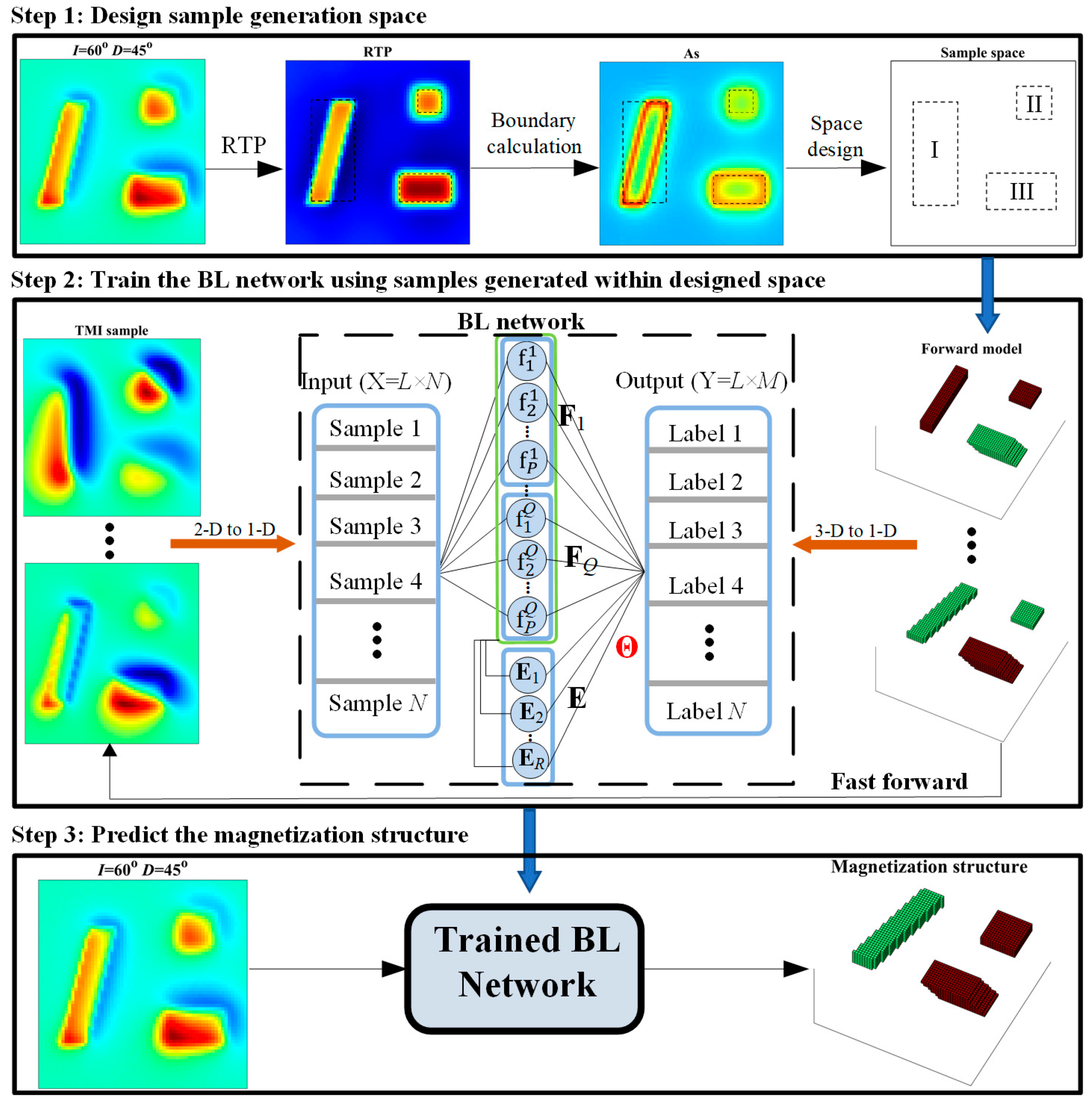
2. Methods
- Step 1: Design the generation space of samples according to the distribution characteristics of TMI.
- Step 2: Establish training samples in the designed generation space. Train the BL network with the samples to obtain the parameter matrix Θ.
- Step 3: Input the field TMI data into the trained BL network to predict the underground magnetization structure.
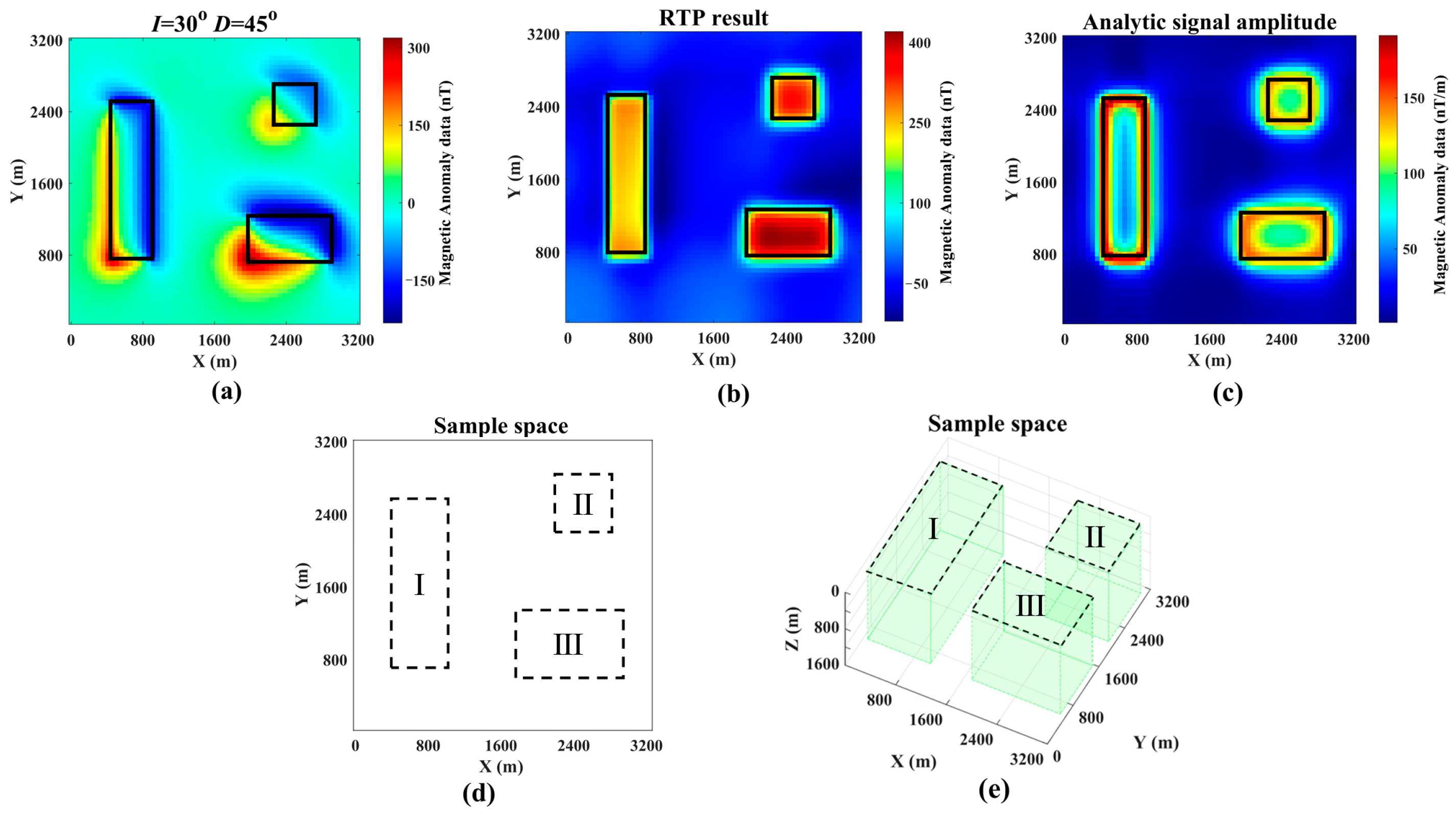
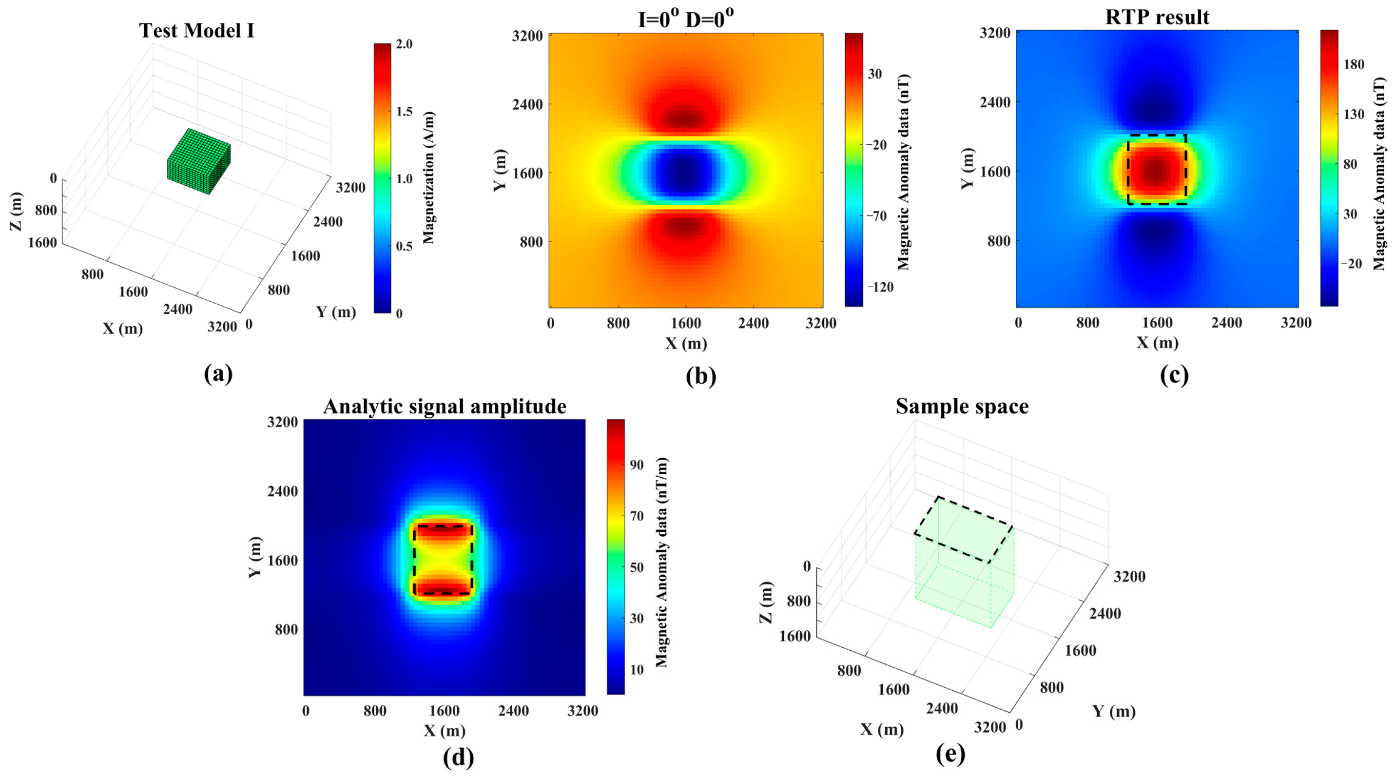
2.1. Sample Generation Space Design
2.2. Sample Generation
2.3. Broad Learning
2.4. Parameter Tuning
3. Results
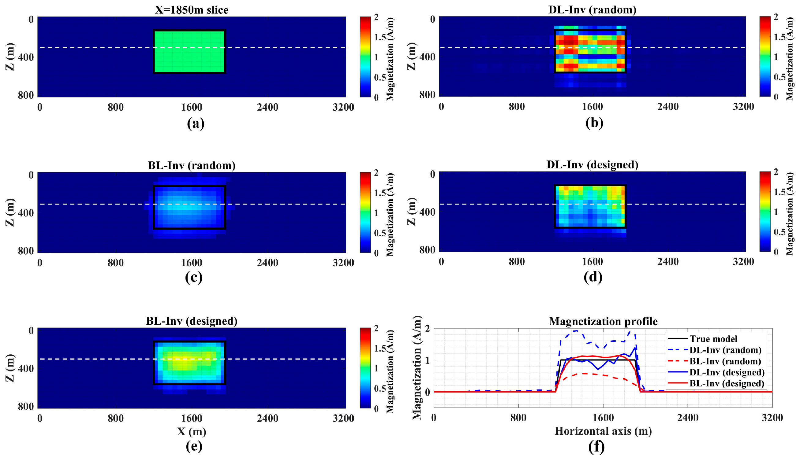
3.1. Synthetic Model I
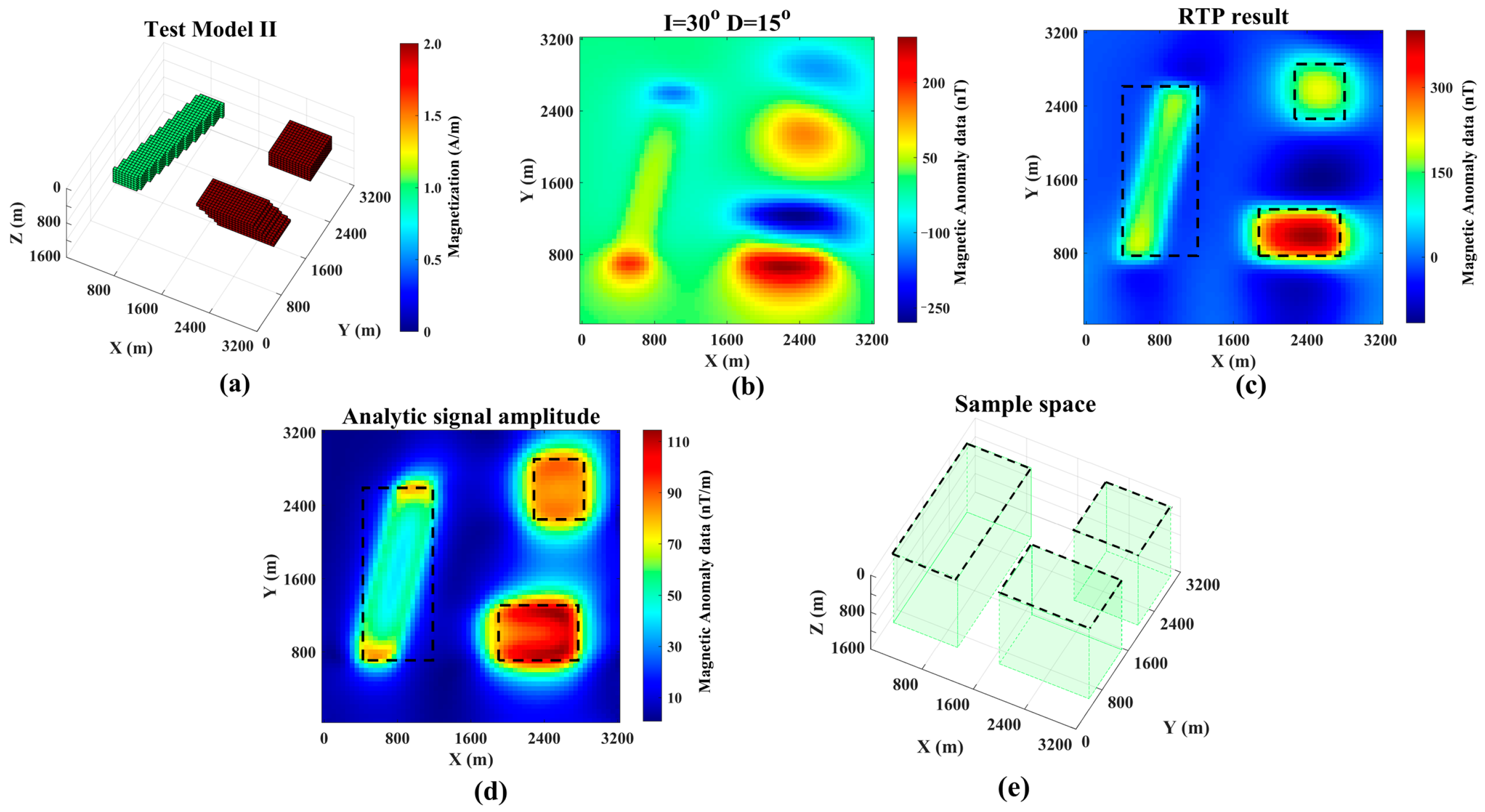
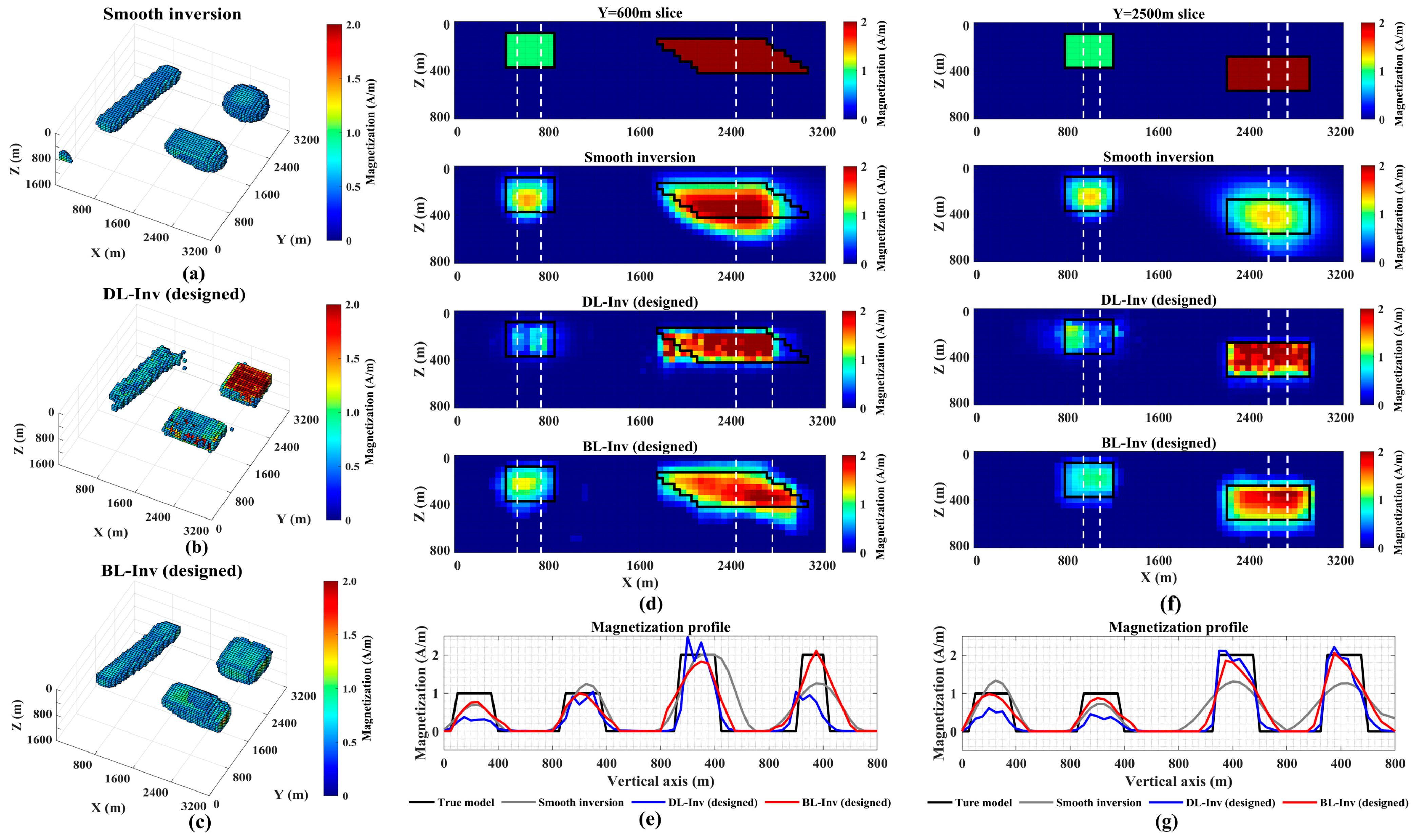
3.2. Synthetic Model II
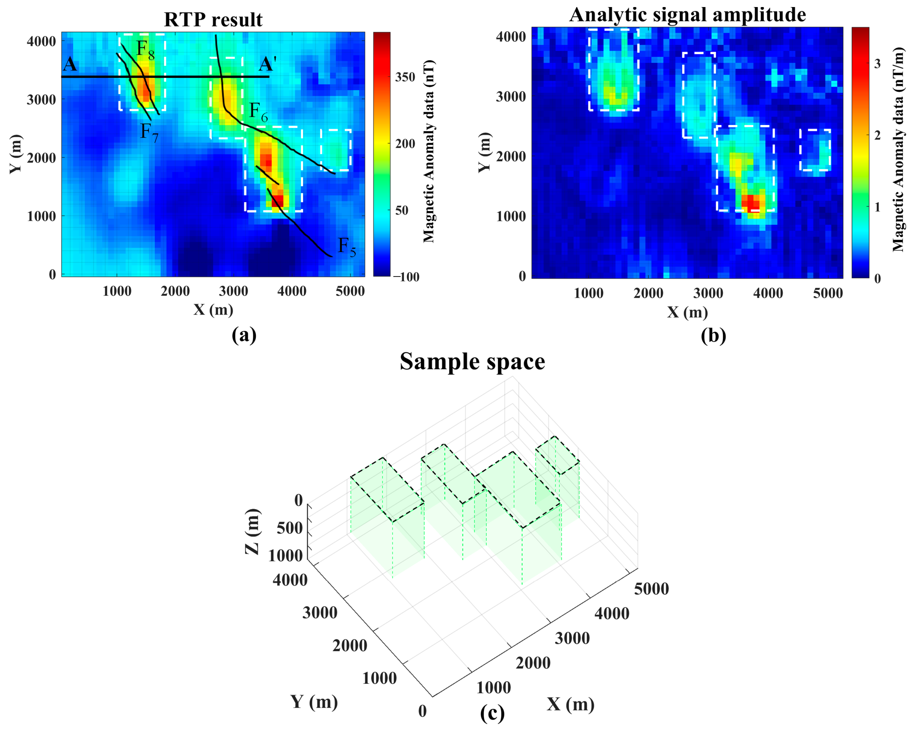
3.3. Field Data Application
4. Discussion
5. Conclusions
Author Contributions
Funding
Data Availability Statement
Acknowledgments
Conflicts of Interest
Abbreviations
| 3-D | Three-dimensional |
| 2-D | Two-dimensional |
| DL | Deep learning |
| BL | Broad learning |
| I | Magnetization inclination |
| D | Magnetization declination |
| TMI | Total magnetic intensity |
| DL-Inv | Deep learning for magnetic 3-D inversion |
| BL-Inv | Broad learning for magnetic 3-D inversion |
| RTP | Reduced-to-the-pole |
| AS | Analytic signal amplitude |
References
- Li, J.; Wang, J.; Meng, X.; Fang, Y.; Li, W.; Yang, S. An Analysis and Interpretation of Magnetic Data of the Qing-Chengzi Deposit in Eastern Liaoning (China) Area: Guide for Structural Identification and Mineral Exploration. Minerals 2024, 14, 1272. [Google Scholar] [CrossRef]
- Walter, C.; Braun, A.; Fotopoulos, G. High-resolution unmanned aerial vehicle aeromagnetic surveys for mineral exploration targets. Geophys. Prospect. 2020, 68, 334–349. [Google Scholar] [CrossRef]
- de Smet, T.S.; Nikulin, A.; Romanzo, N.; Graber, N.; Dietrich, C.; Puliaiev, A. Successful application of drone-based aeromagnetic surveys to locate legacy oil and gas wells in Cattaraugus county, New York. J. Appl. Geophys. 2021, 186, 104250. [Google Scholar] [CrossRef]
- Hojjati-Najafabadi, A.; Mansoorianfar, M.; Liang, T.; Shahin, K.; Karimi-Maleh, H. A review on magnetic sensors for monitoring of hazardous pollutants in water resources. Sci. Total Environ. 2022, 824, 153844. [Google Scholar] [CrossRef]
- Sales, T.J.B.; Martins, S.S. Aeromagnetic geophysical data 3D inversion: Revealing internal and external structures of Morro São João Alkaline Complex, Southeast Brazil. J. S. Am. Earth Sci. 2024, 144, 105008. [Google Scholar] [CrossRef]
- Hrouda, F. Magnetic anisotropy of rocks and its application in geology and geophysics. Surv. Geophys. 1982, 5, 37–82. [Google Scholar] [CrossRef]
- Stocco, S.; Godio, A.; Sambuelli, L. Modelling and compact inversion of magnetic data: A Matlab code. Comput. Geosci. 2009, 35, 2111–2118. [Google Scholar] [CrossRef]
- Liu, S.; Hu, X.; Zhang, H.; Geng, M.; Zuo, B. 3D Magnetization Vector Inversion of Magnetic Data: Improving and Comparing Methods. Pure Appl. Geophys. 2017, 174, 4421–4444. [Google Scholar] [CrossRef]
- Wei, X.; Sun, J. 3D probabilistic geology differentiation based on airborne geophysics, mixed L p norm joint inversion, and physical property measurements. Geophysics 2022, 87, K19–K33. [Google Scholar] [CrossRef]
- Jorgensen, M.; Zhdanov, M.S.; Gribenko, A.; Cox, L.; Sabra, H.E.; Prikhodko, A. 3D Inversion and Interpretation of Airborne Multiphysics Data for Targeting Porphyry System, Flammefjeld, Greenland. Minerals 2024, 14, 1130. [Google Scholar] [CrossRef]
- Hansen, P.C.; O’Leary, D.P. The use of the L-curve in the regularization of discrete ill-posed problems. Siam J. Sci. Comput. 1993, 14, 1487–1503. [Google Scholar] [CrossRef]
- Li, Y.; Oldenburg, D.W. 3-D inversion of magnetic data. Geophysics 1996, 61, 394–408. [Google Scholar] [CrossRef]
- Portniaguine, O.; Zhdanov, M.S. Focusing geophysical inversion images. Geophysics 1999, 64, 874–887. [Google Scholar] [CrossRef]
- Li, Y.; Sun, J. 3D magnetization inversion using fuzzy c-means clustering with application to geology differentiation. Geophysics 2016, 81, J61–J78. [Google Scholar] [CrossRef]
- Fournier, D.; Heagy, L.J.; Oldenburg, D.W. Sparse magnetic vector inversion in spherical coordinates. Geophysics 2020, 85, J33–J49. [Google Scholar] [CrossRef]
- Pilkington, M. 3-D magnetic imaging using conjugate gradients. Geophysics 1997, 62, 1132–1142. [Google Scholar] [CrossRef]
- Li, Y.; Oldenburg, D.W. Fast inversion of large-scale magnetic data using wavelet transforms and a logarithmic barrier method. Geophys. J. Int. 2003, 152, 251–265. [Google Scholar] [CrossRef]
- Liu, S.; Hu, X.; Liu, T. A stochastic inversion method for potential field data; ant colony optimization. Pure Appl. Geophys. 2014, 171, 1531–1555. [Google Scholar] [CrossRef]
- Liu, S.; Liang, M.; Hu, X. Particle swarm optimization inversion of magnetic data: Field examples from iron ore deposits in China. Geophysics 2018, 83, J43–J59. [Google Scholar] [CrossRef]
- Li, Y.; He, Z.; Liu, Y. Application of magnetic amplitude inversion in exploration for volcanic units in a basin environment. Geophysics 2012, 77, B219–B225. [Google Scholar] [CrossRef]
- Li, Z.; Yao, C.; Zheng, Y.; Wang, J.; Zhang, Y. 3D magnetic sparse inversion using an interior-point method. Geophysics 2018, 83, J15–J32. [Google Scholar] [CrossRef]
- Qiang, J.; Zhang, W.; Lu, K.; Chen, L.; Zhu, Y.; Hu, S.; Mao, X. A fast forward algorithm for three-dimensional magnetic anomaly on undulating terrain. J. Appl. Geophys. 2019, 166, 33–41. [Google Scholar] [CrossRef]
- Renaut, R.A.; Hogue, J.D.; Vatankhah, S.; Liu, S. A fast methodology for large-scale focusing inversion of gravity and magnetic data using the structured model matrix and the 2-D fast Fourier transform. Geophys. J. Int. 2020, 223, 1378–1397. [Google Scholar] [CrossRef]
- Vatankhah, S.; Renaut, R.A.; Mickus, K.; Liu, S.; Matende, K. A comparison of the joint and independent inversions for magnetic and gravity data over kimberlites in Botswana. Geophys. Prospect. 2022, 70, 1602–1616. [Google Scholar] [CrossRef]
- Zhou, X.; Chen, Z.; Lv, Y.; Wang, S. 3-D gravity intelligent inversion by U-Net network with data augmentation. IEEE Trans. Geosci. Remote Sens. 2023, 61, 1–13. [Google Scholar] [CrossRef]
- Xue, J.; Huang, Q.; Wu, S.; Nagao, T. LSTM-Autoencoder Network for the Detection of Seismic Electric Signals. IEEE Trans. Geosci. Remote Sens. 2022, 60, 1–12. [Google Scholar] [CrossRef]
- Schuster, G.T.; Chen, Y.; Feng, S. Review of physics-informed machine-learning inversion of geophysical data. Geophysics 2024, 89, T337–T356. [Google Scholar] [CrossRef]
- Ling, W.; Pan, K.; Zhang, J.; He, D.; Zhong, X.; Ren, Z.; Tang, J. A 3-D Magnetotelluric Inversion Method Based on the Joint Data-Driven and Physics-Driven Deep Learning Technology. IEEE Trans. Geosci. Remote Sens. 2024, 62, 1–13. [Google Scholar] [CrossRef]
- Liu, B.; Pang, Y.; Jiang, P.; Liu, Z.; Liu, B.; Zhang, Y.; Cai, Y.; Liu, J. Physics-Driven Deep Learning Inversion for Direct Current Resistivity Survey Data. IEEE Trans. Geosci. Remote Sens. 2023, 61, 1–11. [Google Scholar] [CrossRef]
- Doyoro, Y.G.; Gelena, S.K.; Lin, C. Improving subsurface structural interpretation in complex geological settings through geophysical imaging and machine learning. Eng. Geol. 2025, 344, 107839. [Google Scholar] [CrossRef]
- Geng, Z.; Wu, X.; Shi, Y.; Fomel, S. Deep learning for relative geologic time and seismic horizons. Geophysics 2020, 85, WA87–WA100. [Google Scholar] [CrossRef]
- Yang, Q.; Hu, X.; Liu, S.; Jie, Q.; Wang, H.; Chen, Q. 3-D gravity inversion based on deep convolution neural networks. IEEE Trans. Geosci. Remote Sens. 2021, 19, 1–5. [Google Scholar] [CrossRef]
- Zhang, L.; Zhang, G.; Liu, Y.; Fan, Z. Deep Learning for 3-D Inversion of Gravity Data. IEEE Trans. Geosci. Remote Sens. 2022, 60, 1–18. [Google Scholar] [CrossRef]
- Shi, X.; Jia, Z.; Geng, H.; Liu, S.; Li, Y. Deep Learning Inversion for Multivariate Magnetic Data. IEEE Trans. Geosci. Remote Sens. 2024, 62, 1–10. [Google Scholar] [CrossRef]
- Shi, X.; Wang, Z.; Lu, X.; Cheng, P.; Zhang, L.; Zhao, L. Physics-guided deep learning 3D inversion based on magnetic data. IEEE Trans. Geosci. Remote Sens. 2025, 1, 7500505. [Google Scholar] [CrossRef]
- Hu, Z.; Liu, S.; Hu, X.; Fu, L.; Qu, J.; Wang, H.; Chen, Q. Inversion of magnetic data using deep neural networks. Phys. Earth Planet. Inter. 2021, 311, 106653. [Google Scholar] [CrossRef]
- Jia, Z.; Li, Y.; Wang, Y.; Li, Y.; Jin, S.; Li, Y.; Lu, W. Deep learning for 3-D magnetic inversion. IEEE Trans. Geosci. Remote Sens. 2023, 61, 1–10. [Google Scholar] [CrossRef]
- Li, R.; Yu, N.; Wang, X.; Liu, Y.; Cai, Z.; Wang, E. Model-based synthetic geoelectric sampling for magnetotelluric inversion with deep neural networks. IEEE Trans. Geosci. Remote Sens. 2020, 60, 1–14. [Google Scholar] [CrossRef]
- Chen, C.P.; Liu, Z. Broad learning system: An effective and efficient incremental learning system without the need for deep architecture. IEEE Trans. Neural Netw. Learn. Syst. 2017, 29, 10–24. [Google Scholar] [CrossRef]
- Gao, Z.; Dang, W.; Liu, M.; Guo, W.; Ma, K.; Chen, G. Classification of EEG signals on VEP-based BCI systems with broad learning. IEEE Trans. Syst. Man Cybern. Syst. 2020, 51, 7143–7151. [Google Scholar] [CrossRef]
- Li, W.; Han, M.; Feng, S. Multivariate chaotic time series prediction: Broad learning system based on sparse PCA. In Proceedings of the Neural Information Processing: 25th International Conference, ICONIP 2018, Siem Reap, Cambodia, 13–16 December 2018; Springer: Cham, Switzerland Part VI. ; pp. 56–66. [Google Scholar]
- Yang, X.; Zhou, Y.; Han, P.; Feng, X.; Chen, X. Near-Surface Rayleigh Wave Dispersion Curve Inversion Algorithms: A Comprehensive Comparison. Surv. Geophys. 2024, 45, 773–818. [Google Scholar] [CrossRef]
- Yang, X.; Zu, Q.; Zhou, Y.; Han, P.; Chen, X. A Sample Selection Method for Neural-network-based Rayleigh Wave Inversion. IEEE Trans. Geosci. Remote Sens. 2024, 62, 1–17. [Google Scholar] [CrossRef]
- Yang, X.; Han, P.; Yang, Z.; Miao, M.; Sun, Y.; Chen, X. Broad Learning Framework for Search Space Design in Rayleigh Wave Inversion. IEEE Trans. Geosci. Remote Sens. 2022, 60, 1–17. [Google Scholar] [CrossRef]
- Hu, K.; Ren, H.; Huang, Q.; Zeng, L.; Butler, K.E.; Jougnot, D.; Linde, N.; Holliger, K. Water Table and Permeability Estimation from Multi-Channel Seismoelectric Spectral Ratios. J. Geophys. Res. Solid Earth 2023, 128, e2022JB025505. [Google Scholar] [CrossRef]
- Tao, T.; Han, P.; Yang, X.; Zu, Q.; Hu, K.; Mo, S.; Li, S.; Luo, Q.; He, Z. Fast Initial Model Design for Electrical Resistivity Inversion by Using Broad Learning Framework. Minerals 2024, 14, 184. [Google Scholar] [CrossRef]
- Xu, G.; Zu, Q.; Yang, X.; Tao, T.; Han, P.; Luo, Q.; Han, S.; He, Z. Three-Dimensional Broad Learning Gravity Data Inversion Using Single-Anomaly Training Samples. Appl. Sci. 2024, 14, 11409. [Google Scholar] [CrossRef]
- Li, X. Magnetic reduction-to-the-pole at low latitudes: Observations and considerations. Lead. Edge 2008, 27, 990–1002. [Google Scholar] [CrossRef]
- Ibraheem, I.M.; Tezkan, B.; Bergers, R. Integrated Interpretation of Magnetic and ERT Data to Characterize a Landfill. Pure Appl. Geophys. 2021, 178, 2127–2148. [Google Scholar] [CrossRef]
- Rochette, P.; Jackson, M.; Aubourg, C. Rock magnetism and the interpretation of anisotropy of magnetic susceptibility. Rev. Geophys. 1992, 30, 209–226. [Google Scholar] [CrossRef]
- Clark, D.A. Magnetic effects of hydrothermal alteration in porphyry copper and iron-oxide copper–gold systems: A review. Tectonophysics 2014, 624, 46–65. [Google Scholar] [CrossRef]
- Melo, A.T.; Sun, J.; Li, Y. Geophysical inversions applied to 3D geology characterization of an iron oxide copper-gold deposit in Brazil. Geophysics 2017, 82, K1–K13. [Google Scholar] [CrossRef]
- Rodriguez, J.D.; Perez, A.; Lozano, J.A. Sensitivity Analysis of k-Fold Cross Validation in Prediction Error Estimation. IEEE Trans. Pattern Anal. Mach. Intell. 2010, 32, 569–575. [Google Scholar] [CrossRef]
- Dong, S.; Jiao, J.; Zhou, S.; Lu, P.; Zeng, Z. 3-D Gravity data inversion based on Enhanced Dual U-Net Framework. IEEE Trans. Geosci. Remote Sens. 2023, 61, 1–11. [Google Scholar] [CrossRef]
- MacLeod, I.N.; Jones, K.; Dai, T.F. 3-D analytic signal in the interpretation of total magnetic field data at low magnetic latitudes. Explor. Geophys. 1993, 24, 679–688. [Google Scholar] [CrossRef]
- Xu, Z.; Wang, R.; Zhdanov, M.S.; Wang, X.; Li, J.; Zhang, B.; Liang, S.; Wang, Y. Inversion of the Gravity Gradiometry Data by ResUet Network: An Application in Nordkapp Basin, Barents Sea. IEEE Trans. Geosci. Remote Sens. 2023, 61, 1–10. [Google Scholar] [CrossRef]
- Qiu, H.; Xie, P.; Li, P.; Li, J.; Zhang, X. Application of the integrated ore- prospecting method in the Danzhukeng Pb-Zn-Ag deposit, eastern Guangdong. Geology Explor. 2019, 55, 1394–1403. [Google Scholar] [CrossRef]
- Liu, S.; Hu, X.; Xi, Y.; Liu, T.; Xu, S. 2D sequential inversion of total magnitude and total magnetic anomaly data affected by remanent magnetization. Geophysics 2015, 80, K1–K12. [Google Scholar] [CrossRef]
- Zhang, X.; Li, M. The application of comprehensive geophysical prospecting method to the exploration of polymetallic mine in danzhukeng area. Chin. Eng. Geophys. 2018, 15, 98–103. [Google Scholar] [CrossRef]
- Liu, B.; Guo, Q.; Li, S.; Liu, B.; Ren, Y.; Pang, Y.; Guo, X.; Liu, L.; Jiang, P. Deep learning inversion of electrical resistivity data. IEEE Trans. Geosci. Remote Sens. 2020, 58, 5715–5728. [Google Scholar] [CrossRef]
- Li, Y.; Jia, Z.; Lu, W. Self-Supervised Deep Learning for 3D Gravity Inversion. IEEE Trans. Geosci. Remote Sens. 2022, 60, 1–11. [Google Scholar] [CrossRef]
- Liu, Y.; Wang, J.; Li, W.; Li, F.; Fang, Y.; Meng, X. A Stable Method for Estimating the Derivatives of Potential Field Data Based on Deep Learning. IEEE Trans. Geosci. Remote Sens. 2025, 22, 1–5. [Google Scholar] [CrossRef]
- Zhang, Z.H.; Yao, Y.; Shi, Z.Y.; Wang, H.; Qiao, Z.K.; Wang, S.R.; Qian, L.M.; Du, S.H.; Luo, F.; Liu, W.X. Deep learning for potential field edge detection. Chin. J. Geophys. 2022, 65, 1785–1801. [Google Scholar] [CrossRef]
- Hu, Z.; Liu, S.; Hu, X. 3D inversion of potential field data based on fully convolutional networks. In Proceedings of the SEG International Exposition and Annual Meeting 2021, Denver, CO, USA, 26 September 2021; p. D011S042R004. [Google Scholar]


| Method | B | R2 | Time (h) |
|---|---|---|---|
| DL-Inv (random) | 0.6045 | 0.7757 | 2.33 |
| BL-Inv (random) | 0.5766 | 0.7006 | 0.18 |
| DL-Inv (designed) | 0.3966 | 0.8393 | 2.33 |
| BL-Inv (designed) | 0.4146 | 0.8380 | 0.18 |
| Method | B | R2 | Time (h) |
|---|---|---|---|
| Smooth inversion | 0.6157 | 0.6063 | 1.43 |
| DL-Inv (designed) | 0.5002 | 0.7357 | 2.33 |
| BL-Inv (designed) | 0.4988 | 0.7306 | 0.18 |
| Type | Sample Number | Susceptibility κ (4π × 10−6 SI) | ||
|---|---|---|---|---|
| Max | Min | Mean | ||
| Quartz sandstone | 11 | 11.80 | 1.67 | 3.80 |
| Siltstone | 11 | 12.30 | 1.55 | 3.77 |
| Pb-Zn-Ag ores | 9 | 58.15 | 6.63 | 20.21 |
| Silty slate | 69 | 4414 | 431 | 1547 |
| Pyrrhotite Pb-Zn | 6 | 8374 | 1036 | 3112 |
Disclaimer/Publisher’s Note: The statements, opinions and data contained in all publications are solely those of the individual author(s) and contributor(s) and not of MDPI and/or the editor(s). MDPI and/or the editor(s) disclaim responsibility for any injury to people or property resulting from any ideas, methods, instructions or products referred to in the content. |
© 2025 by the authors. Licensee MDPI, Basel, Switzerland. This article is an open access article distributed under the terms and conditions of the Creative Commons Attribution (CC BY) license (https://creativecommons.org/licenses/by/4.0/).
Share and Cite
Zu, Q.; Han, P.; Wang, P.; Yang, X.-H.; Tao, T.; Zeng, Z.; Bai, G.; Li, R.; Wan, B.; Luo, Q.; et al. Three-Dimensional Magnetic Inversion Based on Broad Learning: An Application to the Danzhukeng Pb-Zn-Ag Deposit in South China. Minerals 2025, 15, 295. https://doi.org/10.3390/min15030295
Zu Q, Han P, Wang P, Yang X-H, Tao T, Zeng Z, Bai G, Li R, Wan B, Luo Q, et al. Three-Dimensional Magnetic Inversion Based on Broad Learning: An Application to the Danzhukeng Pb-Zn-Ag Deposit in South China. Minerals. 2025; 15(3):295. https://doi.org/10.3390/min15030295
Chicago/Turabian StyleZu, Qiang, Peng Han, Peijie Wang, Xiao-Hui Yang, Tao Tao, Zhiyi Zeng, Gexue Bai, Ruidong Li, Baofeng Wan, Qiang Luo, and et al. 2025. "Three-Dimensional Magnetic Inversion Based on Broad Learning: An Application to the Danzhukeng Pb-Zn-Ag Deposit in South China" Minerals 15, no. 3: 295. https://doi.org/10.3390/min15030295
APA StyleZu, Q., Han, P., Wang, P., Yang, X.-H., Tao, T., Zeng, Z., Bai, G., Li, R., Wan, B., Luo, Q., Han, S., & He, Z. (2025). Three-Dimensional Magnetic Inversion Based on Broad Learning: An Application to the Danzhukeng Pb-Zn-Ag Deposit in South China. Minerals, 15(3), 295. https://doi.org/10.3390/min15030295