Automated 3D Multivariate Domaining of a Mine Tailings Deposit Using a Continuity-Aware Geostatistical–AI Workflow

Abstract

Geochemical data from mine tailings are layered, compositional, and noisy, complicating automated domaining. This study introduces a continuity-aware workflow the Geostatistical k-means Recurrent Neural Network (GkRNN) that links compositional preprocessing and geostatistical continuity to sequence learning, allowing depth order and lateral context to influence final domain labels. The workflow begins with a centered log-ratio (CLR) transform, followed by construction of a spectral embedding derived from kernelized direct and cross variograms. Clustering is carried out in this embedded space, and depth sequences are regularized with a hidden Markov model (HMM) model and a long short-term memory (LSTM) network. When applied to a multivariate set of tailing drillholes, stratigraphically coherent zones were obtained, depthwise proportions were stabilized, and vertical as well as lateral semivariograms remained consistent with laminated material. Compared with k-means and Gaussian Mixture baselines, over-segmentation was reduced and the intended layered architecture was recovered in most drillholes. The result is a reproducible domaining workflow that enables clearer grade estimation and more transparent risk evaluation.

1. Introduction

Machine learning (ML) is transforming how geologists interpret the subsurface, enabling fully automated, data-driven workflows that can convert complex assay tables into robust three-dimensional resource models. A particularly compelling application is in mine tailings, where the depositional record mirrors operational history and forms vertical clusters of material as processing and discharge conditions change over time. Unlike deeper ore bodies, tailings are located at or near the surface, making them more accessible and enabling potential reprocessing. These deposits often contain residual concentrations of valuable elements such as copper, cobalt, gold, and rare earth elements (REEs), presenting a significant opportunity for secondary resource recovery. However, they remain chemically reactive and, if mismanaged, can pose serious risks to surrounding water and soil quality [1,2,3,4,5].

As the mining industry places more emphasis on responsible tailing management, robust geochemical data analysis has become central to modern geoscience practice. Comprehensive tailing assays provide critical insights into mineral composition, elemental distributions, and potential contaminants, and they support both re-mining strategies and environmental monitoring, as documented by Gitari et al. [1,2]. At the same time, these datasets are typically large, high-dimensional, and noisy, which stretches the capacities of conventional analytical techniques. In mine planning and tailing re-mining, drillhole data derived from such assays form the basic input for delineating mineralization domains and evaluating secondary material recovery, while spatial clustering of drillhole data based on geochemical or geotechnical attributes supports resource evaluation and operational planning [3,4].

Tailings pose particular difficulties for spatial clustering because they are usually low-grade, exhibit limited spatial continuity, and display marked compositional variability [5]. Their vertical layering reflects changes in processing and discharge through time and generates nonstationary downhole sequences with thin, rapidly alternating beds and sharp campaign contacts, which make it easy for conventional clustering to over-segment zones or overlook true depositional packages [6]. Traditional, semi-manual clustering depends heavily on expert judgment, which introduces subjectivity and inconsistency [7], so there is a growing need for automated, reproducible methods that can handle data intensive tasks with minimal human bias. Recent advances in data analysis provide such tools: automated spatial clustering grounded in ML, deep learning (DL), and geostatistical modeling can reduce subjective choices, improve reproducibility, and align with real-time mining workflows, where continuous data collection and near-term analysis support timely operational adjustments [8,9,10]. For tailing re-mining, integrating geochemical data with automated clustering yields more stable zone definitions, clearer estimates of grade distribution, and a more transparent basis for assessing environmental risk.

In recent years, numerous studies have demonstrated the effectiveness of combining ML, DL, and geostatistics for drilling-based geological interpretations, lithological classification, and resource characterization [11,12,13,14]. Horrocks et al. [15], for instance, showcased automated lithological classification in coal exploration using support vector machines, Naïve Bayes, and artificial neural networks; their methods proved scalable and efficient in Queensland, Australia. In a different geological setting, Wang et al. [16] applied DL models to stream sediment geochemical data for leucogranite exploration in the Himalayan orogen, showing strong spatial clustering performance for rare metal deposits. Moreover, Silversides and Melkumyan [4] leveraged Gaussian processes on measurement-while-drilling data to identify geological boundaries in Australian banded iron formations.

Multi scale structure in drillhole data has been captured using wavelet-based methods, where wavelet transforms were used by Hill et al. [17] to classify lithochemical units and continuous wavelet transforms combined with k-means were applied by to refine boundary detection and reduce misclassification. Building on this time series perspective, recurrence analysis was introduced as a multivariate technique for efficient detection of geological boundaries in mineral exploration boreholes and offshore gas wells [18], and a hybrid scheme combining recurrence analysis with k-means was developed to detect rock boundaries and classify rock types in an iron ore mine [3]. Complementary improvements in boundary correlation and unit mapping were obtained when principal component analysis was applied to multiple well logs in carbonate reservoirs [19], while random forest classifiers integrated with explainable artificial intelligence (AI) achieved over 90% accuracy in lithological mapping of arid crystalline terrains in the Middle [20].

Complementing these time series approaches, Markov models have been used to encode sequential structure and uncertainty in facies sequences and three-dimensional geological models. Deng et al. [21] used a hidden Markov model (HMM) to infer magma flow paths and injection points from a mineralization block model, while Ouyang et al. [22] represented vertical stratigraphic transitions with Markov chains and propagated them via Monte Carlo simulation to quantify uncertainty in three-dimensional surfaces. At the logs and seismic scale, Talarico et al. [23] showed that higher-order Markov chains remain a transparent way to impose realistic facies transition probabilities in seismic-to-facies inversion, even when compared with more flexible Recurrent Neural Networks.

In geostatistical clustering, Fouedjio [24] proposed a hierarchical clustering method for identifying spatially contiguous clusters. This work was later extended by Fouedjio et al. [25] who introduced a spectral clustering approach method tailored to geostatistical data, integrating kernel-based measures of spatial dependence to form contiguous and geologically meaningful clusters, validated on both synthetic and real-world datasets. Related work has also linked AI with geostatistical modeling, where Jalloh et al. [26] combined a feedforward neural network with variogram-based kriging in a mineral sands deposit and van der Grijp et al. [27] applied multiple point statistics with direct sampling in a structurally complex gold deposit, together showing that AI-assisted geostatistics can better capture nonlinear grade patterns, respect spatial continuity, and represent geological uncertainty for mine planning.

Despite these advances, both AI and geostatistics face challenges in spatial clustering. Large datasets can overwhelm geostatistical methods, causing computational bottlenecks and difficulty handling nonstationary or non-normal data. Conversely, AI models often lack inherent physical constraints, risking results that overlook key geological structures and spatial continuity [26,28,29].

To address these issues, this paper introduces the Geostatistical k-means Recurrent Neural Network (GkRNN), which combines k-means clustering, spatial continuity from geostatistical analysis, and sequence modeling to produce an automated, spatially informed interpretation of mine tailing data. The following sections present the study site and dataset, outline the workflow, assess geological consistency and operational relevance against k-means and Gaussian Mixture baselines, and conclude with key limitations, practical implications, and directions for future work.

2. Materials and Methods

2.1. Dataset

In this study, a synthetic mining dataset was used to emulate a multivariate geochemical survey from 82 tailing drillholes. This controlled case allows the underlying geological structure, grade variability, and noise characteristics to be specified explicitly, which is useful for isolating the behavior of the GkRNN workflow and benchmarking its internal components without confidentiality constraints.

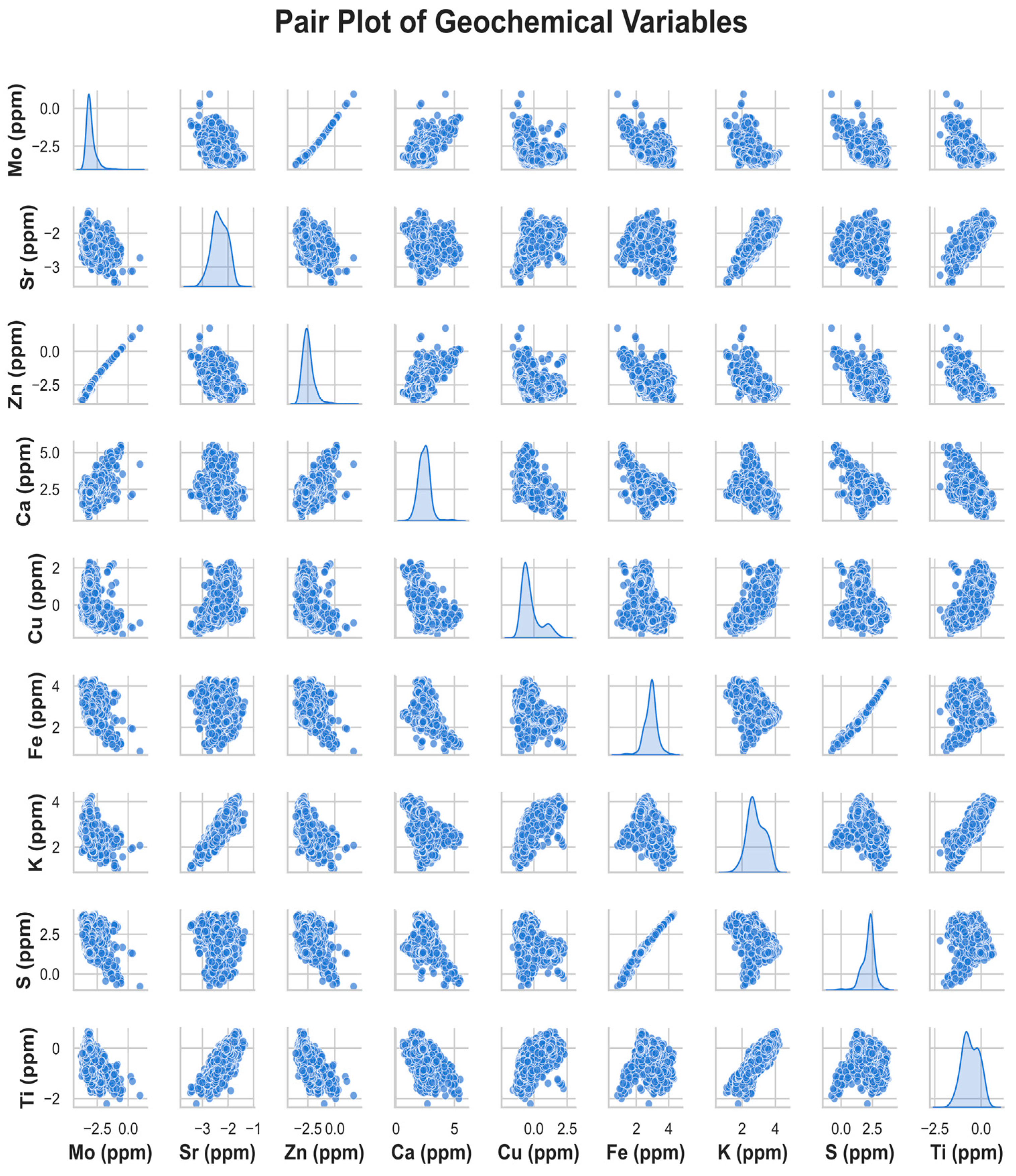
Nine elements were analyzed: molybdenum (Mo), strontium (Sr), zinc (Zn), calcium (Ca), copper (Cu), iron (Fe), potassium (K), sulfur (S), and titanium (Ti). All concentrations were measured in parts per million (ppm). Figure 1 presents a pair plot illustrating the distribution (diagonal histograms) and bivariate relationships (off-diagonal scatter plots) among these elements. The diagonal histograms indicate that Sr, Zn, and S have more pronounced tails, which suggests skewed or possibly multimodal distributions, whereas Ca and K appear closer to approximately normal behavior. The off-diagonal scatter plots show that Ti and Fe form relatively strong linear trends, which is consistent with shared mineralogical sources. In contrast, Cu and K display weaker correlations, which suggests more variable geochemical controls or the influence of multiple phases on their concentrations.

Mo is observed to form distinct clusters, which may reflect the ore processing history or different oxidation states within the tailings [30]. Sr is moderately correlated with Ca, which points to common carbonate- or sulfate-bearing phases [31,32], while the positive relationship between S and Fe is consistent with sulfide mineralization or secondary iron–sulfate compounds [33,34]. Zn tends to overlap with other base metals such as Cu, indicating potential co-occurrence in sulfide or oxide assemblages [35]. Taken together, these patterns highlight the compositional heterogeneity of the tailings and provide a useful basis for designing resource recovery strategies and for assessing environmental risks.

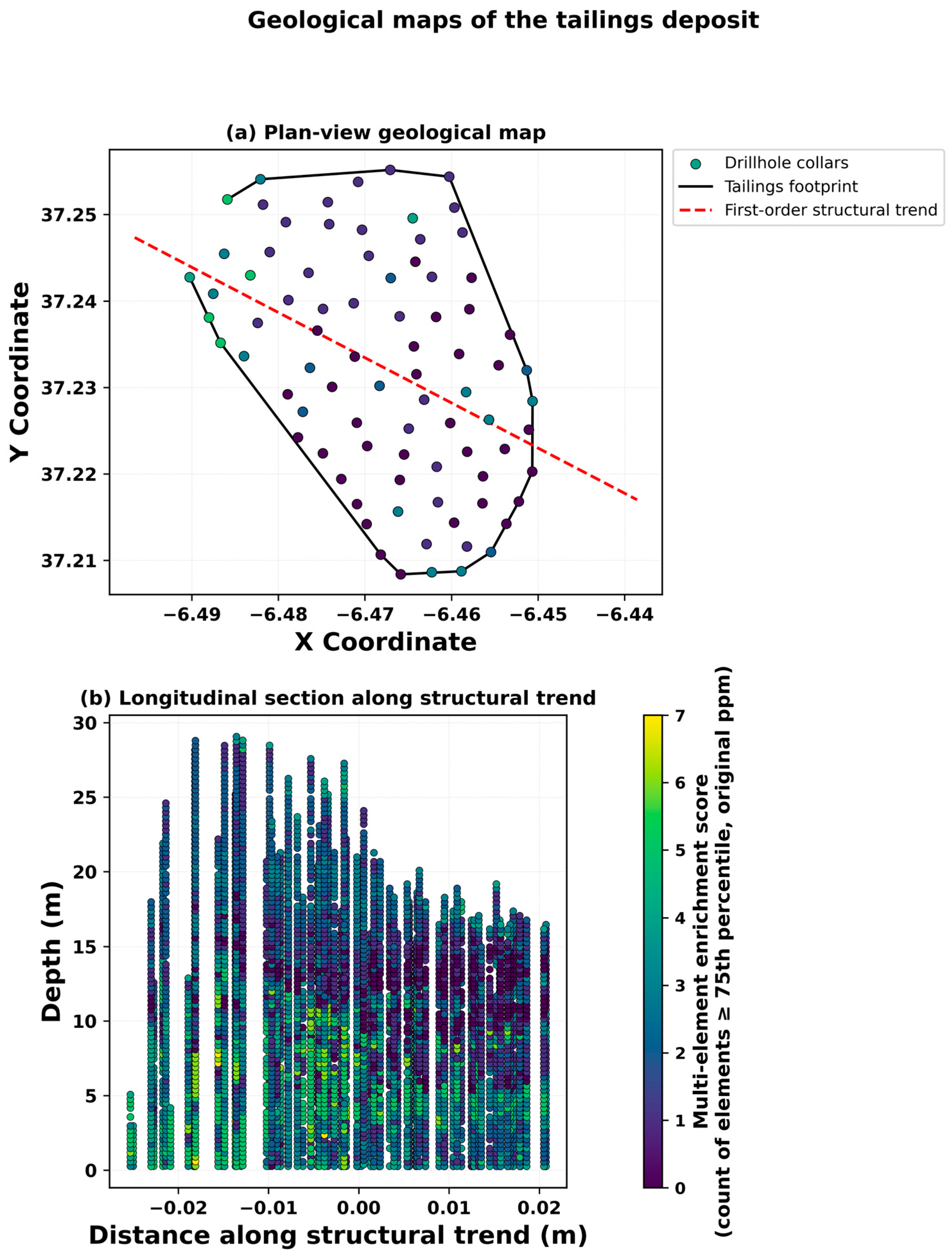
To place the drillhole dataset in its deposit scale context, Figure 2 shows geological maps of the tailing body in plan view and as a longitudinal section along the main structural trend. In the plan view, the tailing footprint is outlined and a first-order structural trend is inferred from the collar geometry. Each collar is colored by a multielement enrichment score that is computed from the original Mo to Ti assays and used as a qualitative indicator of local resource potential. The longitudinal section displays the same enrichment score as a function of distance along the trend and depth, which emphasizes the stacked and stratified character that is expected for operational tailing deposition. Together, these two views summarize the overall geometry, structural framework, and spatial distribution of potentially recoverable material in the study deposit.

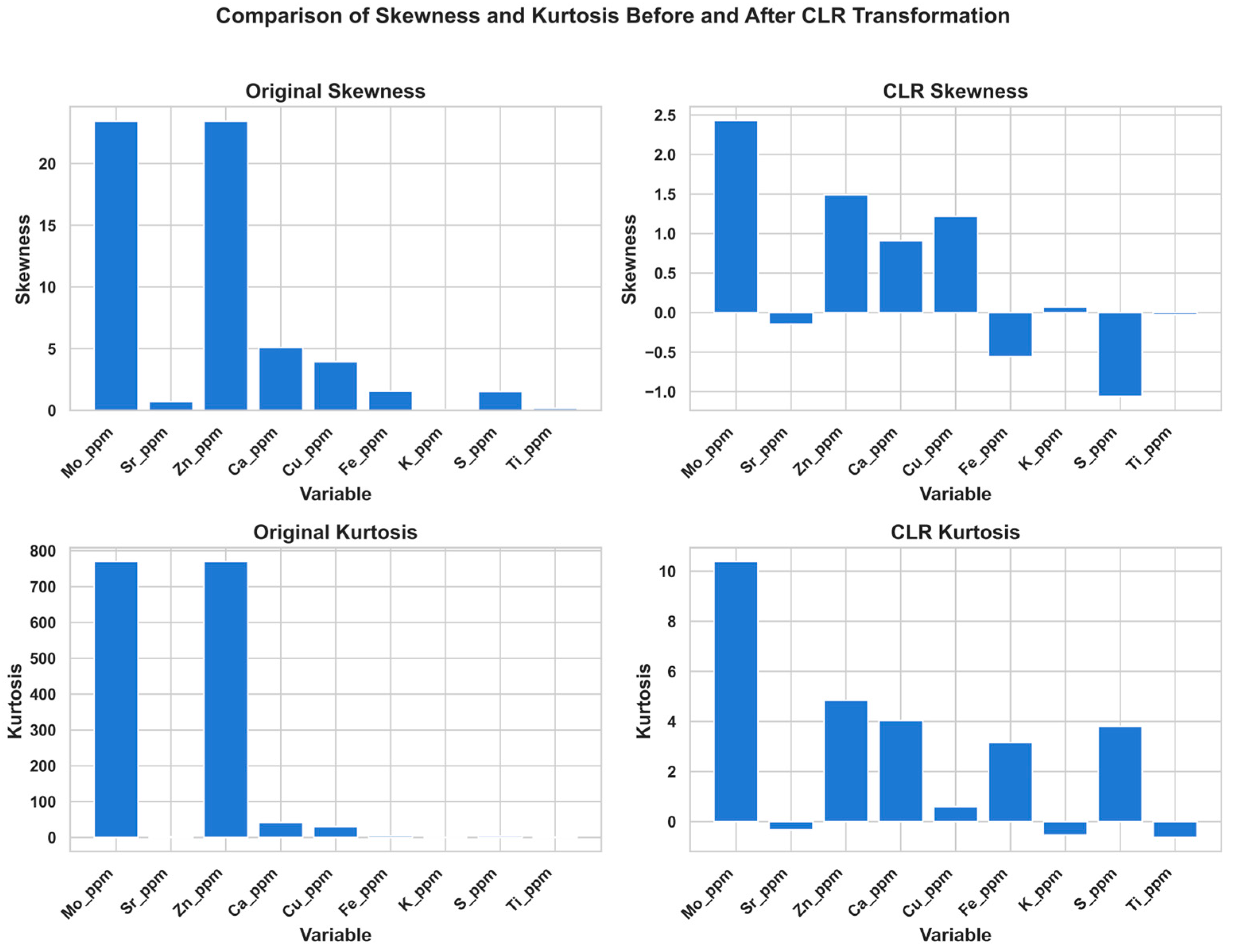
To clarify the statistical effect of compositional preprocessing, skewness and kurtosis were calculated for the nine geochemical variables before and after application of the centered log-ratio (CLR) transformation (Figure 3). In the original data, Mo, Zn, and Ca are strongly right-skewed and display extreme kurtosis, with Mo and Zn showing skewness values above 20 and kurtosis values greater than 750. Such heavy tails can distort standard multivariate analyses and clustering results. This behavior is characteristic of compositional datasets, in which an increase in one component implies a relative decrease in others and can introduce spurious correlations and misleading patterns in the untransformed space.

After the CLR transformation, all variables appear more nearly symmetric. Skewness is markedly reduced and is centered closer to zero, and kurtosis is compressed into a more interpretable range, generally between about 0 and 10. The most extreme tails are therefore dampened, and the multivariate structure of the dataset becomes more suitable for clustering and for a range of machine learning algorithms [30]. Features that previously dominated the variance, such as Mo and Zn, now have magnitudes that are more comparable to those of elements such as Fe, K, and Ti. This rebalancing allows each geochemical component to contribute more evenly to dimensionality reduction and clustering, which in turn enhances interpretability and confidence in subsequent spatial and statistical modeling.

2.2. Methodology

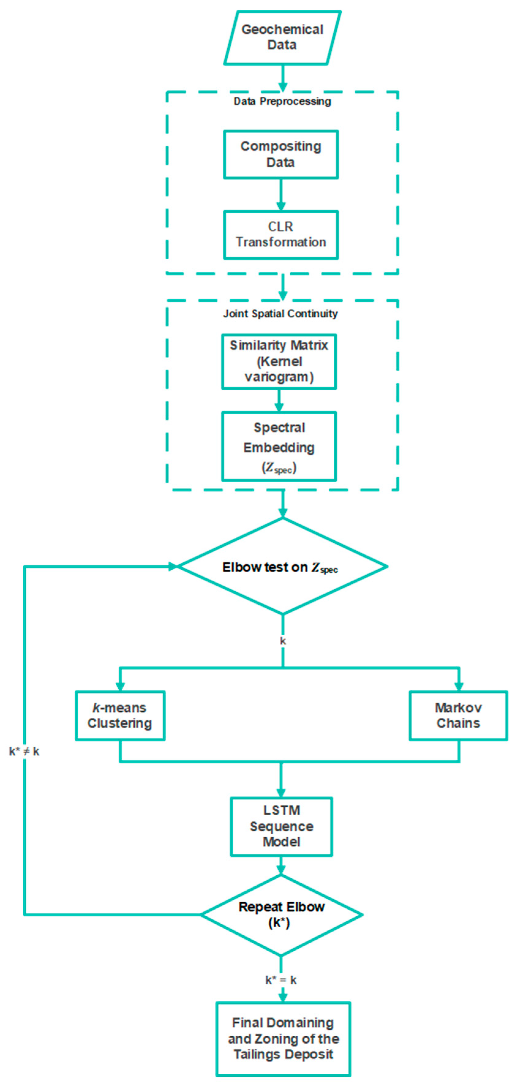
The GkRNN workflow (Figure 4) begins with preparation of the geochemical logs so that downhole profiles can be compared consistently across boreholes. Irregular assays are first composited to constant depth intervals. The composited data are then transformed with the CLR transformation so that each element is treated as a part of a whole, which allows mult ielement relationships to be analyzed in a proportional and comparable way.

In the next stage, joint spatial continuity is characterized. Direct and cross variograms of the CLR variables are used to construct a lag-dependent variogram matrix, which is converted into a similarity measure. A simple spatial proximity term is added so that samples that are close together in space retain a strong relationship. A spectral embedding of the resulting affinity matrix provides a compact set of coordinates that summarize joint continuity. An elbow analysis on these coordinates is then used to select a parsimonious number of clusters k, and k-means clustering in the embedded space yields provisional labels that already reflect both geochemical affinity and lateral context.

Depthwise structure is then imposed through two sequence models so that the final domains respect the way tailings are stacked through time. First, the cluster labels are ordered from shallow to deep and a left-to-right Markov chain is fitted to adjacent downhole transitions. An HMM that uses either the leading spectral coordinates or the CLR features as emissions is then applied to smooth each borehole sequence and to reduce rapid back jumps that would break the expected stratigraphic order. Second, a Recurrent Neural Network with long short-term memory (LSTM) units is trained on sliding depth windows. Each time step is represented by an augmented feature vector that combines normalized coordinates, spectral descriptors, distances to spectral centroids, and a local continuity score. During training, a consistency term encourages the LSTM transitions to remain compatible with the learned Markov structure, and overlapping windows vote at each depth position to stabilize the boundaries.

In the final step, the smoothed sequences are converted into practical domains. A minimum thickness criterion is applied so that extremely thin intervals are merged according to the learned transition preferences. Each borehole is then restricted to at most four contiguous units in order to preserve operational simplicity and stratigraphic plausibility. If the elbow diagnostic suggests a different value of k, the loop is repeated. The final output is a set of depth-ordered, laterally coherent zones assigned to every sample and borehole, which provides a compact and geologically sensible domaining of the tailing deposit.

2.2.1. Data Preprocessing

Compositing Downhole Assays into Uniform Intervals

Downhole assays were first composited into uniform intervals. For each borehole, samples were sorted by depth and partitioned into contiguous left-closed intervals of 0.3 m that covered the sampled range. Elemental concentrations within each interval were then aggregated as depth-weighted means, using the recorded sample thicknesses, so that mass balance was preserved under irregular sampling. Across all boreholes, this procedure produced a single table of uniformly spaced 0.3 m slices that was used for consistent downstream analysis. Intervals with no observations were omitted in order to avoid the introduction of artificial values. Each composite retained its start, end, and midpoint depths so that the downhole chronology and spatial positioning remained clearly defined in subsequent stages of the workflow.

CLR Transformation of Compositional Data

The resulting geochemical data are compositional, because the components convey relative information and sum to a constant total, such as 100 percent or a fixed mass. This situation is typical in geochemical applications, where concentrations reported in parts per million need to be interpreted in a proportional rather than absolute sense. The constant sum constraint creates dependence among components and can lead to spurious correlations, since an increase in one component must be offset by relative decreases in others. As a consequence, conventional Euclidean distances may not provide a reliable measure of dissimilarity, and standard multivariate methods can produce misleading patterns when they are applied directly to raw compositions [36,37].

To overcome these obstacles, log ratio transformations have been introduced as a means to open the data and render it amenable to standard statistical techniques. Among these, the CLR transformation is particularly popular. For a compositional vector $x$ = ($x$₁, $x$₂, …, $x$_D) in ${\mathbb{R}}^D$, where $D$ denotes the number of geochemical components and each $x_{i }$is strictly positive, the CLR transformation is defined on a component-wise basis by Equation (1):

$$z_i=\ln \left({\displaystyle \frac{x_i}{g\left(x\right)}}\right), i=1,2,\cdots ,D$$

(1)

where $g\left(x\right)$ represents the geometric mean of the components:

$$g\left(x\right)={\left(\prod _{j=1}^D{x}_j\right)}^{{\displaystyle \frac{1}{D}}}=\exp \left({\displaystyle \frac{1}{D}}\sum _{j=1}^D\mathrm{l}\mathrm{n}\left(x_j\right)\right)$$

(2)

The original composition can be recovered, up to a constant factor, by applying the element-wise exponential to a CLR vector and normalizing across components, which is equivalent to the softmax mapping that is widely used in ML.

By normalizing each component with the geometric mean and then applying the natural logarithm, the CLR transformation centers the data so that the transformed components satisfy the constraint $\sum _{i=1}^D{z}_i=0$. In this way, the constant sum constraint is removed and closure effects, together with the false correlations they induce, are reduced. The compositions are mapped into an ordinary Euclidean space, where relationships between elements can be compared in a more neutral way, and the resulting variables can be used directly in standard geostatistical models and many machine learning algorithms that assume real valued, unconstrained inputs. A nonlinear pre autoencoding step could in principle also be used to learn a low-dimensional representation of the compositions with similar aims, but in this study the CLR is preferred because its statistical behavior is well-understood and it has already been widely used in compositional geoscience applications.

2.2.2. Joint Spatial Continuity

In geostatistics, spatial dependence among observations is often described through measures of joint spatial continuity, which characterize how multiple variables co-vary as a function of distance [24,25,38,39]. Direct and cross variograms are traditionally used as the main tools for describing second-moment dependence [40]. However, when the data are high-dimensional or exhibit complex distributional behavior, classical variogram modeling may not capture all relevant structures. To address this limitation, a non-parametric measure of joint continuity is adopted in this study, based on pairwise comparisons of empirical increments. This approach preserves second-moment information, such as variances and covariances, while remaining flexible with respect to non-Gaussian and multivariate complexity.

Let Z(x) ∈${\mathbb{R}}^p$ denote the vector of $p$ CLR-transformed geochemical variables at a spatial location x∈$\mathbb{R}$³, observed at sites $\{x_i{\}}_{i=1}^n$. Building on previous work in geostatistical clustering, a lag-dependent variogram matrix is estimated in order to encode both direct and cross continuity in a single positive semi-definite (PSD) object, which is then converted into a data-adaptive similarity.

A kernel variogram matrix is first constructed. For a set of lag centers $\{{\mathit{r}}_{\mathit{g}}{\}}_{\mathit{g}=1}^{\mathit{L}}$ that span the empirical range of inter-sample spacings, the separation between two samples at locations ${\mathit{x}}_{\mathit{i}}$ and ${\mathit{x}}_{\mathit{j}}$ is defined as ${\mathit{r}}_{\mathit{i}\mathit{j}}=|{\mathit{x}}_{\mathit{i}}-{\mathit{x}}_{\mathit{j}}|.$ For each lag center ${\mathit{r}}_{\mathit{g}}$, a Gaussian kernel weight is assigned,

$$w_{ij}\left(r_g\right)=\exp \left\{-{\displaystyle \frac{1}{2}}{\left({\displaystyle \frac{r_{ij}-r_g}{b}}\right)}^2\right\}$$

(3)

where $b > 0$ is a bandwidth parameter that is chosen in relation to the median neighbor spacing. These weights give more influence to pairs whose separation is close to the target lag.

Writing $\Delta Z_{ij}=Z\left(x_i\right)-Z\left(x_j\right)$, the kernelized direct and cross semivariograms at lag $r_g$ are estimated as

$$\left\{\begin{array}{c}{\widehat{\mathsf{\gamma }}}_{\mathrm{u}\mathrm{v}}\left(r_g\right)={\displaystyle \frac{{\sum }_{i<j}{w}_{ij}\left(r_g\right)\hspace{0.17em}\Delta Z_{ij}^{\left(u\right)}\hspace{0.17em}\Delta Z_{ij}^{\left(v\right)}}{2{\sum }_{i<j}{w}_{ij}\left(r_g\right)}},\hspace{1em}u,v=1,\dots ,p\\ \widehat{\mathrm{\Gamma }}\left(r_g\right)=diag\left(\widehat{{\gamma }_{11}},\dots ,\widehat{{\gamma }_{pp}}\right)-{\left[{\widehat{\mathsf{\gamma }}}_{\mathrm{u}\mathrm{v}}\left(r_g\right)\right]}_{u\ne v}\end{array}\right.$$

(4)

where $\Delta Z_{ij,u}$ and $\Delta Z_{ij,v}$ denote the $u$-th and $v$-th components of the increment $\Delta Z_{ij}$.

Because sampling noise can lead to small negative eigenvalues, a PSD correction is applied. Let $V\mathsf{\Lambda }{V}^{\mathrm{\top }}$ be the eigendecomposition of Γ$\left(r_g\right)$. A PSD-regularized matrix is then obtained as follows:

$${\widehat{\mathrm{\Gamma }}}_{\mathrm{p}\mathrm{s}\mathrm{d}}\left(r_g\right)=\mathrm{V}\hspace{0.17em}\max \left(\mathsf{\Lambda },0\right)\hspace{0.17em}{V}^{\mathrm{\top }}+\mathrm{\epsilon }{I}_p, \mathrm{\epsilon }\simeq {10}^{-6}$$

(5)

where the operator $\max \left(\mathsf{\Lambda },0\right)$ replaces any negative eigenvalues by zero and $\mathrm{\epsilon }{I}_p$ provides a small ridge term for numerical stability. This step ensures that each ${\widehat{\mathrm{\Gamma }}}_{\mathrm{p}\mathrm{s}\mathrm{d}}\left(r_g\right)$ is positive semi-definite.

A distance-aware dissimilarity is then derived from the joint continuity structure. For a pair of samples ($i,j$) with separation $r_{ij}$, the matrix ${\widehat{\mathrm{\Gamma }}}_{\mathrm{p}\mathrm{s}\mathrm{d}}\left(r_{ij}\right)$ is obtained by linearly interpolating the PSD-corrected matrices between the neighboring lag centers that bracket $r_{ij}$. A squared dissimilarity is defined as weight increments by the inverse of the continuity matrix,

$$d_{ij}^2=\Delta Z_{ij}^{\mathrm{\top }}\hspace{0.17em}{\widehat{\Gamma }}_{\mathrm{psd}}^{-1}\left(r_{ij}\right)\hspace{0.17em}\Delta Z_{ij}$$

(6)

Small values of $d_{ij}^2$ indicate behavior that is consistent with local joint continuity at that separation, whereas large values flag atypical increments at that distance.

These dissimilarities are then converted to similarities on a sparse local proximity graph formed by short-range pairs. For edges ($i,j$) in this graph, the similarity is defined as follows:

$$\left\{\begin{array}{c}{s}_{ij}=\exp \left(-{\displaystyle \frac{d_{ij}^2}{\tau }}\right)\\ \tau =median\{d_{ij}^2\hspace{0.25em}\mathrm{o}\mathrm{v}\mathrm{e}\mathrm{r} \mathrm{g}\mathrm{r}\mathrm{a}\mathrm{p}\mathrm{h} \mathrm{e}\mathrm{d}\mathrm{g}\mathrm{e}\mathrm{s}\}\end{array}\right.$$

(7)

where the scale parameter τ is chosen as the median of the squared dissimilarities over all graph edges. This choice allows the similarity values to be well-conditioned and robust to heterogeneous variance across different datasets.

The joint continuity affinity matrix $S_{\mathrm{vario}}=\left[s_{ij}\right]$ The joint continuity affinity matrix $A_{\mathrm{spat}}$ is obtained by applying a Gaussian kernel of Euclidean distance to the same short-range pairs. The final affinity matrix is given by

$$A=w_{\mathrm{vario}}\hspace{0.17em}{S}_{\mathrm{vario}}+w_{\mathrm{spat}}\hspace{0.17em}{A}_{\mathrm{spat}}$$

(8)

where $w_{\mathrm{vario}}$ and $w_{\mathrm{spat}}$ are non-negative weights that control the relative influence of the variogram-based and purely spatial terms. In this construction, $A\in {\mathbb{R}}^{n\times n}$ is a symmetric, sparse affinity matrix whose rows and columns index the samples. Each entry $A_{ij}\ge 0$combines information about joint geochemical continuity and geometric proximity, so that larger values indicate a stronger local similarity between samples $i$ and $j$, whereas zero entries correspond to pairs that are not treated as neighbors. The weights $w_{\mathrm{v}\mathrm{a}\mathrm{r}\mathrm{i}\mathrm{o}}$ and $w_{\mathrm{s}\mathrm{p}\mathrm{a}\mathrm{t}}$ control the relative influence of the variogram-based and purely spatial terms. This matrix serves as the adjacency of the graph used in the subsequent spectral embedding step and is the main input from which continuity-aware clustering features are derived.

Although the case study uses nine elements, the GkRNN architecture are not tied to this dimensionality and can accommodate larger multivariate assays. Numerical stability is maintained by operating on standardized CLR variables, regularizing the variogram matrices (kernel smoothing and PSD correction), and projecting them into a fixed low-dimensional spectral space for clustering and sequence learning. The main practical requirement is that the number of samples remains sufficiently larger than the number of variables for reliable variogram and emission estimation, and very high-dimensional assays may be screened or reduced without changing the model structure.

2.2.3. Elbow Method for Determining Optimal Clusters

In spatial cluster analysis, particularly when k-means clustering is used, the choice of the number of clusters k is crucial for obtaining a segmentation that is both interpretable and geologically meaningful. A common heuristic for this purpose is the elbow method, which relies on the idea of within-cluster dispersion to identify the point at which increasing k no longer produces a substantial gain in compactness [3].

The key quantity in the elbow method is the inertia, denoted by $I\left(k\right)$. Inertia measures how tightly the data points in each cluster are grouped around their respective centroids. For a dataset with $N$ points, the inertia for a given value of k is defined as follows [41,42]:

$$I\left(k\right)=\sum _{i=1}^N{‖x_i-{\mu }_{c_i}‖}^2$$

(9)

where $x_i$ is the feature vector of the i-th sample in the clustering space, ${\mu }_{c_i}$ is the centroid of the cluster $c_i$ to which $x_i$ is assigned, and ‖⋅‖ denotes the Euclidean norm. Thus, each term ${‖x_i-{\mu }_{c_i}‖}^2$ represents the squared distance from a sample to the center of its cluster, and $I\left(k\right)$ aggregates this quantity over all samples. Smaller values of $I\left(k\right)$ indicate more compact clusters in the chosen feature space.

In practice, the number of clusters is varied from 1 up to a preselected maximum, and the corresponding values of $I\left(k\right)$ are computed for each k. These inertia values are then plotted against k to produce an elbow plot. The chosen value of k is taken at the point where the curve begins to flatten, so that further increases in the number of clusters yield only modest reductions in inertia and are therefore less likely to provide additional interpretive value.

2.2.4. K-Means Clustering

k-means clustering is a widely adopted unsupervised learning algorithm designed to partition N observations into k distinct clusters by minimizing the sum of squared distances between each data point and the nearest cluster centroid. This goal is mathematically represented by the objective function as follows [41]:

$$\underset{\left\{{\mathsf{\mu }}_c\right\},\left\{c_i\right\}}{\min }\sum _{i=1}^N{‖x_i-{\mu }_{c_i}‖}^2$$

(10)

where $x_i$ denotes the i-th observation, and ${\mu }_{C_i}$ is the centroid of the cluster to which $x_i$ is assigned. The algorithm operates through an iterative process that alternates between two main steps. In the first, known as the assignment step, each data point is allocated to the cluster corresponding to the closest centroid, effectively grouping similar observations based on Euclidean distance. Following this, the update step recalculates the centroids by computing the mean of the points assigned to each cluster. This cycle of assigning data points and updating centroids continues until the process converges, meaning there are minimal changes in the assignments or the reduction in the overall sum of squared distances becomes negligible. Through this systematic refinement, k-means clustering effectively reveals the underlying structure of the data, thereby providing a robust tool for segmentation and pattern recognition in diverse scientific applications [41,42,43].

2.2.5. Markov Chains

After graph-based clustering and depthwise relabeling, sequence regularization along each borehole was carried out by fitting a first-order Markov model to the provisional zone labels. Within each borehole, samples were ordered by depth and a left-to-right indexing was imposed so that forward progression corresponded to non-decreasing state indices. Transition frequencies were counted from all adjacent depth pairs, and domain transitions were constrained so that geologically implausible back jumps (that is, transitions to lower indices) were discouraged [44]. Smoothing was then performed with an HMM whose emissions were taken from the first D coordinates of the spectral features Z_spec. In this way, the sequence model remained consistent with the joint continuity structure encoded earlier in the kernel variogram affinity.

Let $C_{ij}$ denote the count of observed transitions $i \to j$ along depth across all boreholes after left-to-right relabeling. Let $M_{ij}\in \left\{\mathrm{0,1}\right\}$ indicate whether a transition from state $i$ to state $j$ is permitted under the geological constraints. For example, one can take $M_{ij}=0$ for back jumps with $j<i$. If a strictly absorbing last state k is used, this is implemented by setting${ M}_{k,k}=1 \mathrm{a}\mathrm{n}\mathrm{d} M_{k,j}=0$ for all $j\ne k$. With a small Dirichlet ridge parameter $\mathrm{\alpha }> 0$, t a row-normalized transition matrix $P=\left[P_{ij}\right]$ is obtained as follows:

$$P_{ij}={\displaystyle \frac{C_{ij}+\mathrm{\alpha }{M}_{ij}}{{\sum }_{j^{\prime }}\left(C_{i{j}^{\prime }}+\mathrm{\alpha }{M}_{i{j}^{\prime }}\right)}}$$

(11)

This normalization yields a valid stochastic matrix whose rows represent smoothed transition probabilities that respect the allowed moves encoded in $M_{ij}$.

For each state $j$, the emission likelihood is modeled as a multivariate normal distribution with diagonal covariance, estimated from the samples currently assigned to state $j$. Writing $x_t\in {\mathbb{R}}^{D_e}$for the chosen feature vector at depth index t, and ${\mathrm{\mu }}_j, \mathrm{and} \hspace{0.25em}{\mathrm{\Sigma }}_j=diag\left({\mathrm{\sigma }}_{j1}^2,\dots ,{\mathrm{\sigma }}_{j{D}_e}^2\right)$ for the state specific mean and variances, the likelihood can be written as follows:

$$b_j\left(x_t\right)=\mathcal{N}\left(x_t∣{\mu }_j,{\mathrm{\Sigma }}_j\right)={\displaystyle \frac{exp\left(-\frac{1}{2}{\sum }_{d=1}^{D_e}\frac{{\left(x_{td}-{\mu }_{jd}\right)}^2}{{\sigma }_{jd}^2}\right)}{{\left(2\pi \right)}^{D_e/2{\prod }_{d=1}^{D_e}{\sigma }_{jd}}}}$$

(12)

where $x_{td}$ denotes the d-th component of $x_t$, ${\mu }_{jd}$ is the corresponding mean for state $j$, and ${\sigma }_{jd}^2$ is the associated variance. The numerator measures how far the feature vector lies from the state mean in each dimension, scaled by the variance, while the denominator ensures proper normalization of the density.

Given an empirical initial distribution ${\mathrm{\pi }}_0,$ formed from the first labels in each borehole, maximum a posteriori state sequences are computed independently for each borehole using the Viterbi dynamic program in log space. Let ${\delta }_t\left(j\right)$ denote the best log score of any path ending in state j at depth index t. The recursion is as follows:

$$\left\{\begin{array}{c}{\delta }_t\left(j\right)=\underset{i}{\max }\left\{{\delta }_{t-1}\left(i\right)+\log P_{ij}\right\}+\log b_j\left(x_t\right),\\ {\delta }_1\left(j\right)=\log {\pi }_0\left(j\right)+\log b_j\left(x_1\right)\end{array}\right.$$

(13)

At each depth, the algorithm keeps track of the most likely predecessor state, and backtracking from the final time step yields the most probable smoothed sequence of domains for each borehole.

2.2.6. RNN Architecture and Feature Integration

Depthwise regularities in the clustered geochemical logs were modeled using an LSTM-based Recurrent Neural Network. Fixed-length windows were extracted for each borehole, and each time step t was represented by an augmented feature vector combining normalized spatial coordinates, graph-spectral descriptors, distances to spectral centroids, and a local continuity score. Let $\widetilde{x_t},\hspace{0.25em}\widetilde{y_t},\hspace{0.25em}\widetilde{z_t}$ denote min–max normalized coordinates, $Z_{spec}\left(t\right)\in {\mathbb{R}}^{D_z}$ the spectral embedding, $\{{\mathrm{\mu }}_c{\}}_{c=1}^k$ the spectral space centroids, and $S_{\mathrm{loc}}\left(t\right)$ the mean graph similarity at the sample location; the per-step input was then defined as follows:

$$\left\{\begin{array}{c}{x}_t={\left[\hspace{0.17em}\widetilde{z_t},\hspace{0.25em}\widetilde{x_t},\hspace{0.25em}\widetilde{y_t},\hspace{0.25em}{Z}_{\mathrm{spec}}^{\left(1:3\right)}\left(t\right),\hspace{0.25em}{d}_1\left(t\right),\dots ,d_k\left(t\right),\hspace{0.25em}{S}_{\mathrm{loc}}\left(t\right)\hspace{0.17em}\right]}^{\mathrm{\top }},\\ d_c\left(t\right)=\Vert Z_{\mathrm{spec}}\left(t\right)-{\mu }_c{\Vert }_2\end{array}\right.$$

(14)

where $Z_{\mathrm{spec}}^{\left(1:3\right)}\left(t\right)$ denotes the first three spectral coordinates, which capture the dominant structure of the embedding, and the remaining components summarize proximity to cluster centers and local graph continuity.

Temporal dependencies in these inputs are modeled using standard LSTM dynamics. With σ(⋅) denoting the logistic sigmoid function and ⊙ denoting the element-wise product, the input gate $i_t$, forget gate $f_t$, output gate $o_t$, candidate cell state $\widetilde{c_t}$, cell state $c_t$, and hidden state $h_t$ evolve as follows:

$$\begin{gathered} i_t=\sigma \left(W_i{x}_t+U_i{h}_{t-1}+b_i\right) \\ {f}_t=\sigma \left(W_f{x}_t+U_f{h}_{t-1}+b_f\right) \\ {o}_t=\sigma \left(W_o{x}_t+U_o{h}_{t-1}+b_o\right) \\ \widetilde{c_t}=f_t\odot c_{t-1}+i_t\odot \widetilde{c_t} \\ { h}_t=o_t\odot \tanh \left(c_t\right) \end{gathered}$$

(15)

In these expressions, the matrices $W_i,W_f,W_o,W_c$ and $U_i,U_f,U_o,U_c$ and the vectors $b_i,b_f,b_o,b_c$ are trainable parameters. The input gate controls how much new information from $x_t$ enters the cell, the forget gate determines how much of the previous cell state $c_{t-1}$ is retained, and the output gate regulates how much of the updated cell state is exposed through $h_t$.

At each time step, the hidden state is mapped to class probabilities through a time-distributed softmax layer as follows:

$$y_t=\mathrm{softmax}\left(W_h{h}_t+b_h\right)\in {\mathrm{\Delta }}^{k-1}$$

(16)

where $W_h$and $b_h$ are trainable parameters and ${\mathrm{\Delta }}^{k-1}$ denotes the probability simplex over the k domain classes. The vector $y_t$ therefore defines a probability distribution over the domain labels at depth t, converting the hidden state into a probabilistic prediction of the target classes [45]. Alignment with stratigraphic progression is described qualitatively in this subsection. The network’s inferred transitions are compared with an HMM structure, and consistency with that structure is encouraged elsewhere in the pipeline, without the need for additional formal equations here.

2.2.7. Combined GkRNN Framework

Assays are first composited to fixed depth intervals and then transformed using the CLR so that the geochemical variables are placed on a common compositional scale. A sparse affinity matrix A is then constructed by combining a joint continuity term, derived from kernelized lag-dependent direct and cross variograms of the CLR variables, with a geometric proximity term based on short-range spatial pairs. A spectral embedding of A provides the features used for clustering. The elbow method is applied to select the number of clusters k, k-means clustering yields provisional labels, and these classes are reordered from shallow to deep in order to follow the inferred stratigraphy. A left-to-right HMM is subsequently used to regularize depthwise transitions with diagonal Gaussian emissions, and an LSTM trained on short depth windows with a Markov consistency term learns the remaining sequence patterns along the boreholes. The overall GkRNN procedure is summarized as pseudo-code in Algorithm 1.

Algorithm 1: Pseudo-code of GkRNN

Input. Data table; list of geochemical columns geochem_cols; hole identifier id_col; coordinates xyz_cols; configuration parameters cfg. Composite irregular assays to a fixed depth step Δz and keep the within-hole order. Apply the CLR transform to the composited geochemistry and assemble a working table T = [id, X, Y, Z, CLR]. From (X, Y, Z), form short-range spatial pairs and compute their separation distances r(i, j). On a lag grid {r_g}, estimate kernelized direct and cross-variogram matrices Γ(r_g). Stabilize and invert them to obtain Γ_psd−1(r_g) as described in Equations (4) and (5). For each short-range pair (i, j), compute the squared Mahalanobis distance d2(i, j) using Equation (6), and set S_vario(i, j) = exp(−d2(i, j)/τ), with τ defined in Equation (7). Build the geometric adjacency matrix A_spat by applying a Gaussian kernel of Euclidean distance to the same set of short-range pairs. Form the joint affinity matrix A = w_vario · S_vario + w_spat · A_spat, then symmetrize A and set its diagonal entries. Compute the spectral embedding Z_spec from the normalized graph Laplacian of A, with embedding dimension given by cfg.spectral_dim. Select the number of clusters k by applying the elbow method to Z_spec. Run k-means in the embedded space to obtain initial labels labels_0 and cluster centroids. Reorder the labels by class median depth so that state indices increase with depth, yielding left-to-right labels, labels_lr. Count depth-adjacent transitions per hole from labels_lr. Apply the forward constraint and Dirichlet smoothing to obtain the transition matrix P. Choose the emission features (either the first D components of Z_spec or the CLR variables). Fit diagonal Gaussian parameters for each state and run the Viterbi algorithm per hole to obtain HMM-smoothed labels, labels_hmm. Build sliding depth windows. For each time step, construct feature vectors from normalized coordinates, the first three spectral components, distances to the spectral centroids, and a local continuity statistic. Use labels_hmm as training targets. Define an LSTM network with two stacked layers (128 and 64 units, return_sequences = True) followed by a time-distributed dense layer with k outputs. Use a loss that combines cross-entropy with a Markov consistency term based on P. Train the network with early stopping. Apply the trained model with overlapping windows and majority voting to obtain RNN-smoothed labels, labels_lstm. Enforce a minimum thickness rule by merging intervals that are thinner than a chosen threshold, guided by the transition matrix P. Enforce a per-hole cap on the number of contiguous zones (at most four) to obtain the final labels, labels_final. Output. Final zone labels labels_final, transition matrix P, and selected number of clusters k.

3. Results

The GkRNN workflow was applied to a multivariate, CLR-transformed geochemical dataset from 82 tailing drillholes. Clustering was carried out in a spectral space that encodes joint spatial continuity, and the resulting depthwise labels were subsequently regularized through an HMM layer and an LSTM network that was trained to remain consistent with the learned transition structure. In combination, these steps produced a small number of stratigraphically coherent zones in each drillhole that follow the depositional layering and suppress thin, noise-driven oscillations.

3.1. Determination of the Global Cluster Number by a Continuity-Aware Spectral Elbow Criterion

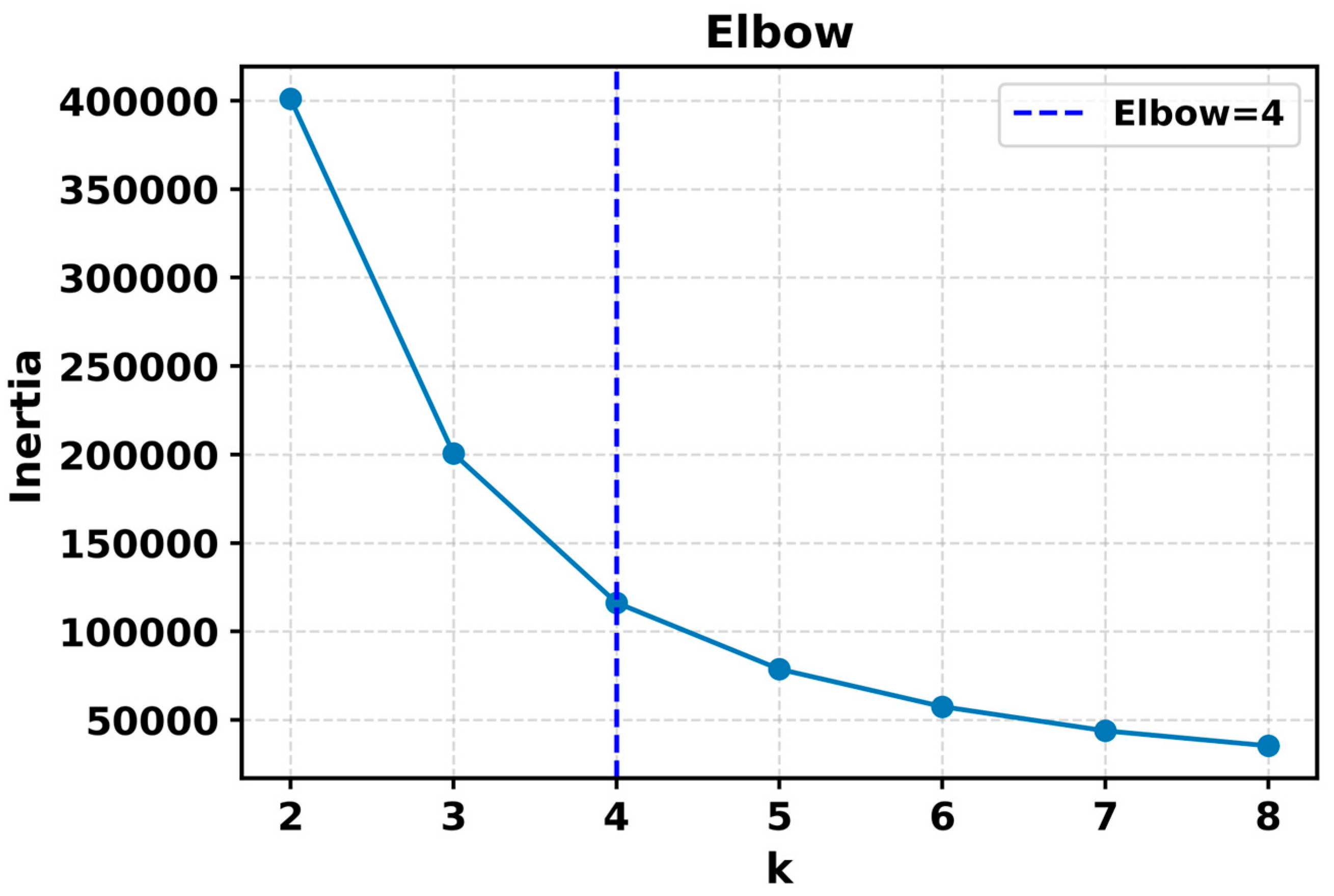
A model selection analysis was undertaken to identify a number of clusters k that is both parsimonious and expressive for the tailings deposit. The procedure operated in a continuity-aware spectral space $Z_{\mathrm{spec}}$that was derived from a joint similarity graph blending a multivariate, kernel variogram-based geochemical affinity with a spatial nearest neighbor term. The normalized graph Laplacian was eigendecomposed to obtain $Z_{\mathrm{spec}}$ (ten leading coordinates), and k-means clustering was performed for candidate values k ∈ [2,8]. For each value of k, the within-cluster inertia was recorded. This quantity decreases as clusters become more internally homogeneous, but typically exhibits diminishing improvements as k increases.

The elbow location was identified using the maximum distance to chord rule, which selects the value of k that has the largest perpendicular distance from the straight line connecting the endpoints of the inertia curve. As shown in Figure 5, a pronounced change in slope occurs at k = 4. Beyond this point, inertia decreases only slowly, which indicates that additional clusters would mainly subdivide existing regimes rather than reveal new, geologically meaningful structure. Accordingly, k = 4 was adopted as the global cluster count for subsequent depthwise regularization and sequence modeling. This choice balances compositional coherence with model simplicity and is consistent with the expected convex decay behavior of inertia in continuity-aware embeddings of tailing data.

3.2. Delineation of Multivariate Compositional Domains Using Continuity-Aware Spectral Clustering

A continuity-aware spectral representation was constructed from a joint similarity graph that combined a kernel variogram-based geochemical affinity with a spatial nearest neighbor term. K-means clustering was applied to the leading spectral coordinates, and the resulting labels were interpreted as depth sequences. These sequences were regularized with a left-to-right HMM and with an LSTM trained on sliding windows that contained normalized coordinates, leading spectral coordinates, distances to class centroids, and a local similarity score. After sequence learning, a minimum thickness rule was applied to remove very thin, non-persistent runs. Unless stated otherwise, a discrete viridis palette is used throughout, and the figures show the final sequence consistent zones.

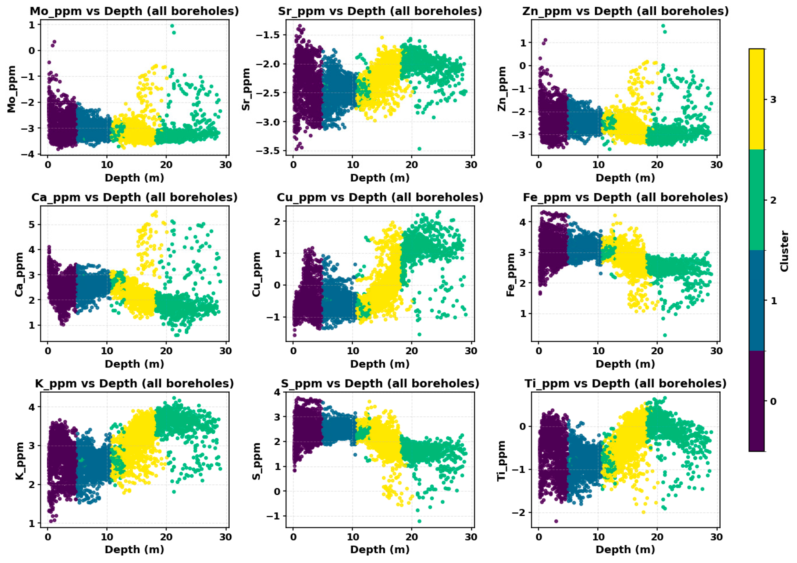
The overall multivariate structure can be examined in the variables-versus-depth mosaic for the tailing deposit, where nine elements (Mo, Sr, Zn, Ca, Cu, Fe, K, S, Ti) are plotted against depth and colored by zone (Figure 6). Bands of similar color appear at comparable depths from hole to hole, which indicates that the zones represent coherent stratification rather than isolated classifications. Element-specific banding is most pronounced for Sr, Zn, Fe, and K, so these tracers contribute most strongly to boundary definition, whereas the remaining variables exhibit more gradual contrasts that describe transitional behavior.

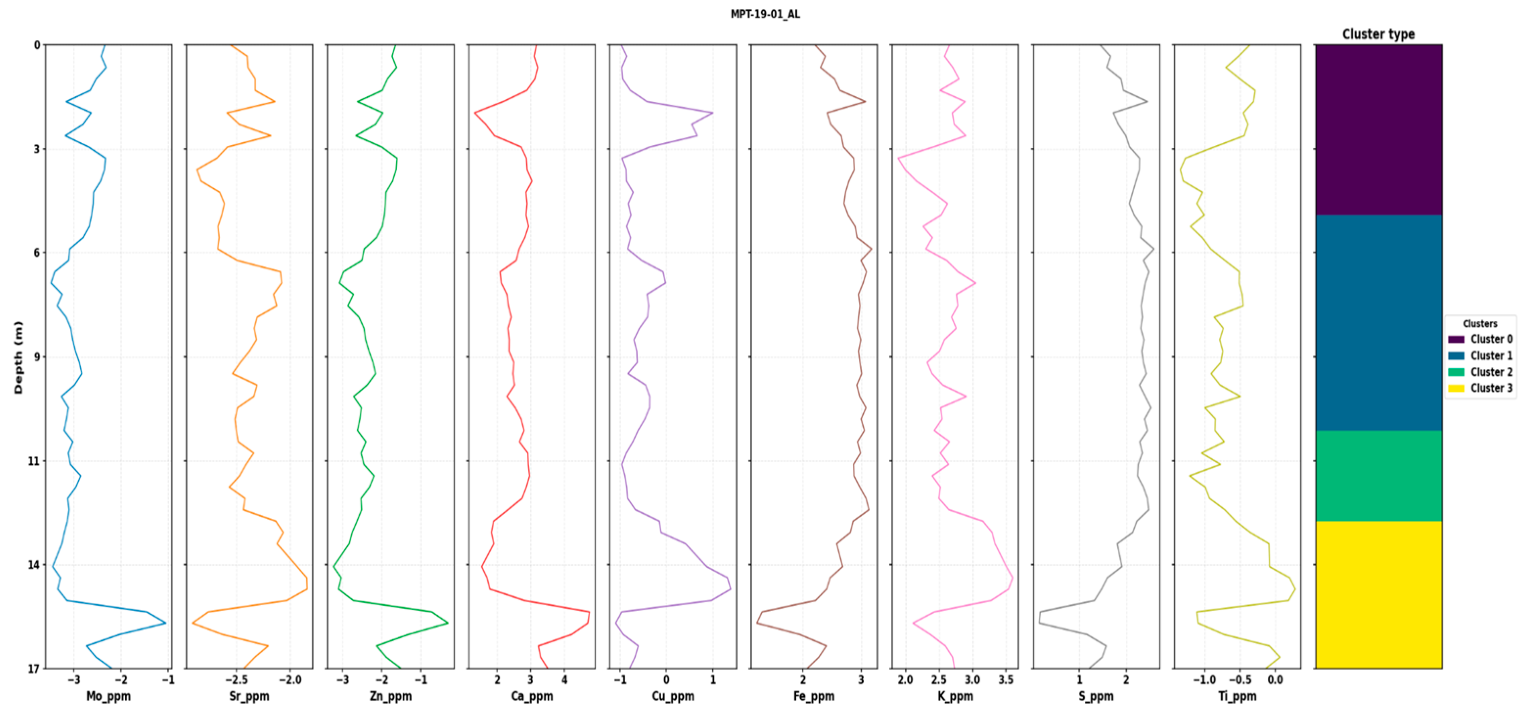
Consistency at the single-hole scale was investigated using borehole MPT 19 01_AL, where nine elemental logs are plotted against depth with a zone strip at the right margin (Figure 7). Depth increases downward, and each trace retains a fixed color by variable. Changes in composition align closely with label transitions, and boundaries appear stable rather than alternating rapidly. One zone displays intermediate values across several elements and acts as a transitional layer between enriched and depleted intervals. The visual agreement between compositional breaks and the contiguous color blocks in the zone strip suggests that the sequence-aware labeling captured persistent units rather than pointwise noise.

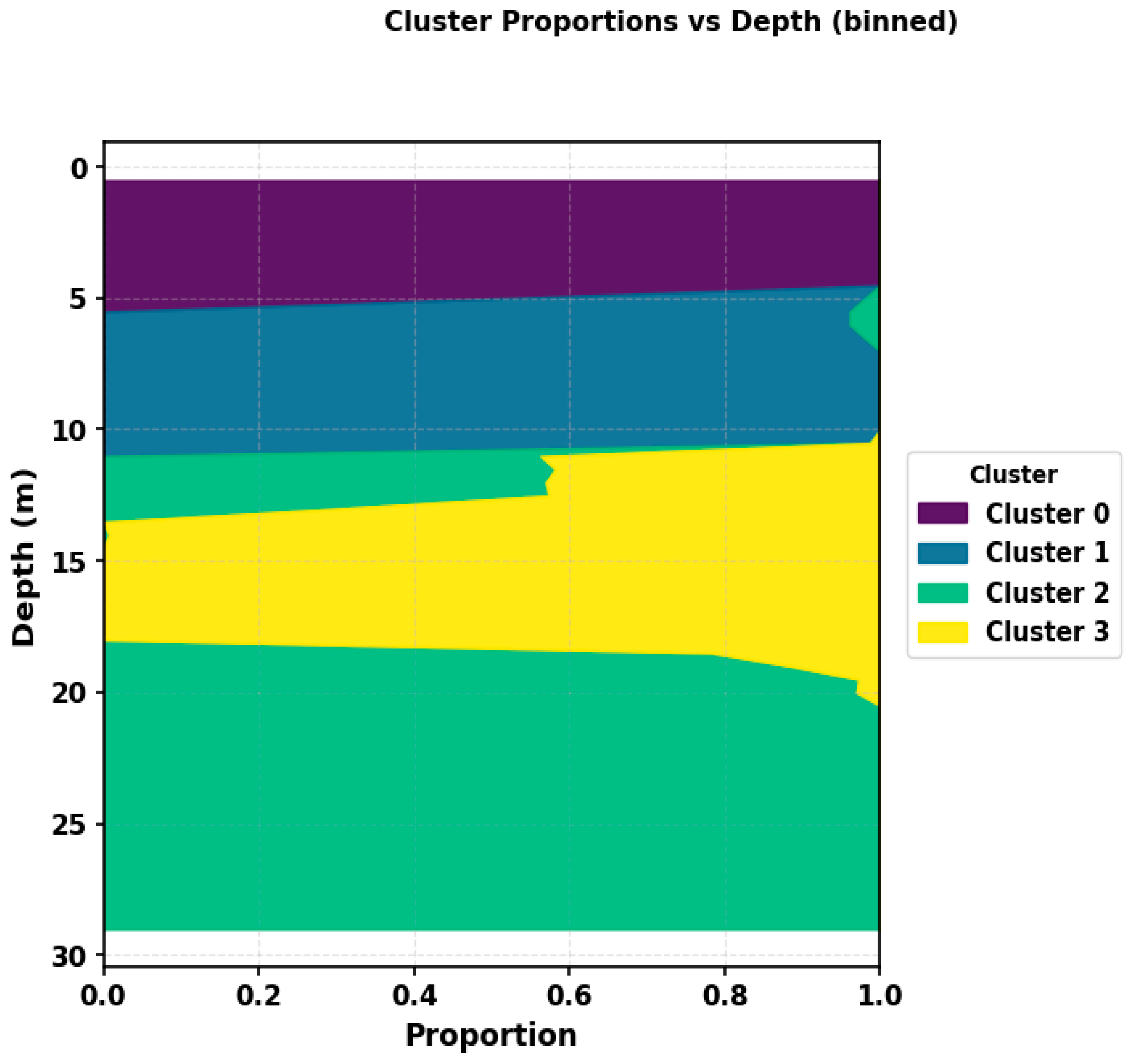
Deposit scale stacking was then summarized using depth binned zone proportions computed at 0.5 m resolution for the tailings deposit (Figure 8). At each depth the stacked ribbons sum to one, and the vertical axis increases downward. A gradual shift can be seen: shallow intervals contain larger proportions of zones 0 and 1, the proportion of the intermediate zone rises through the middle part of the profile, and the deepest section is dominated by zone 2. The smooth trajectories of the ribbons and the absence of abrupt reversals indicate that the labels evolve as a depth-ordered time series rather than as scattered classifications. In this sense, the GkRNN workflow respects the time series character of the tailing deposit, because the Markov and LSTM components learn persistence and transition patterns that govern how zones appear and change with depth.

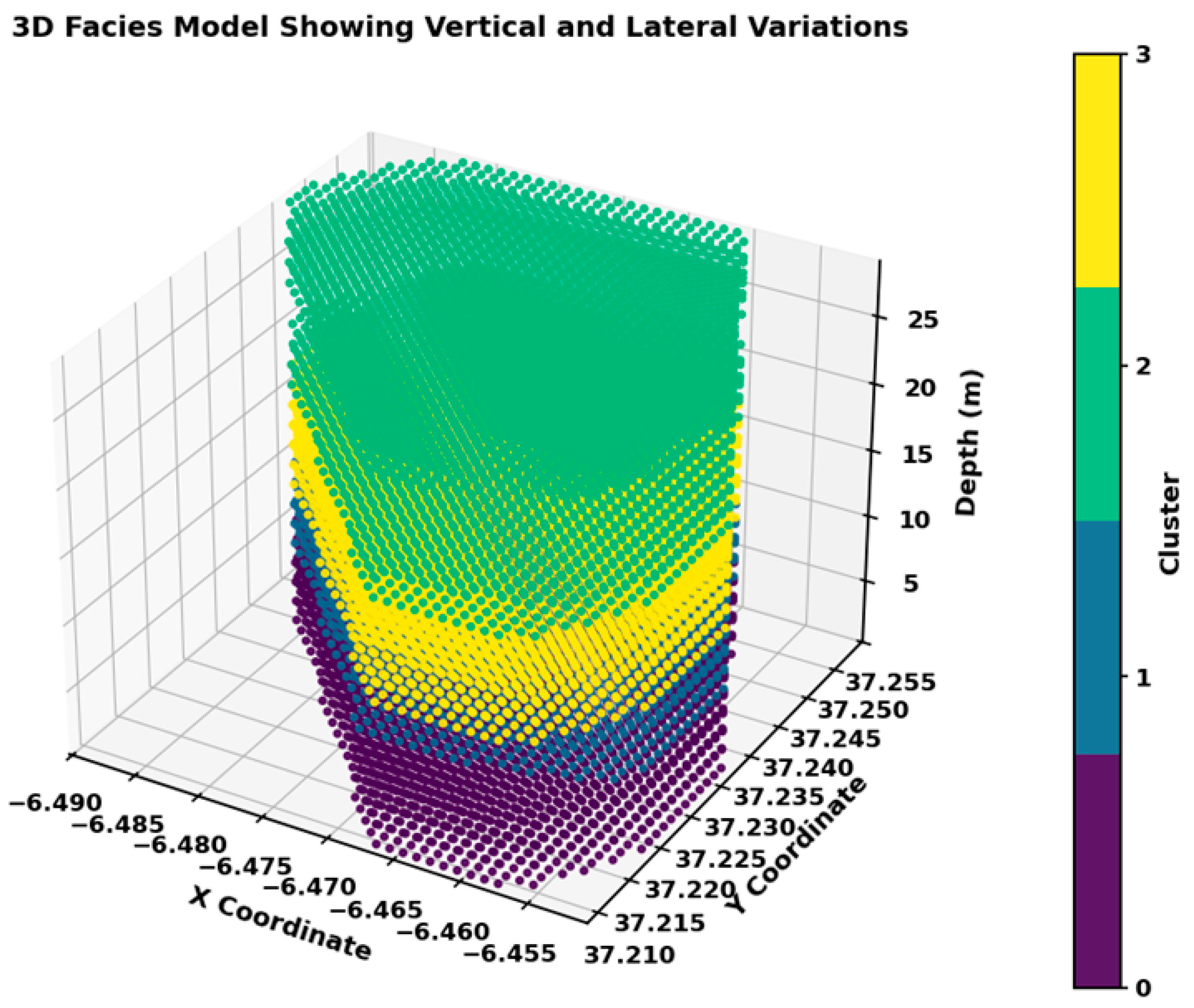
To complement this depth binned view, a 3D facies model was interpolated on a regular grid restricted to the convex hull of the boreholes (Figure 9). Within this footprint, the final GkRNN zones form laterally continuous layers between drillholes and display vertical transitions that are consistent with the depth binned proportions in Figure 8. This 3D representation shows both vertical and lateral facies variations in a single image and confirms that the workflow produces a coherent volumetric domaining of the tailing deposit.

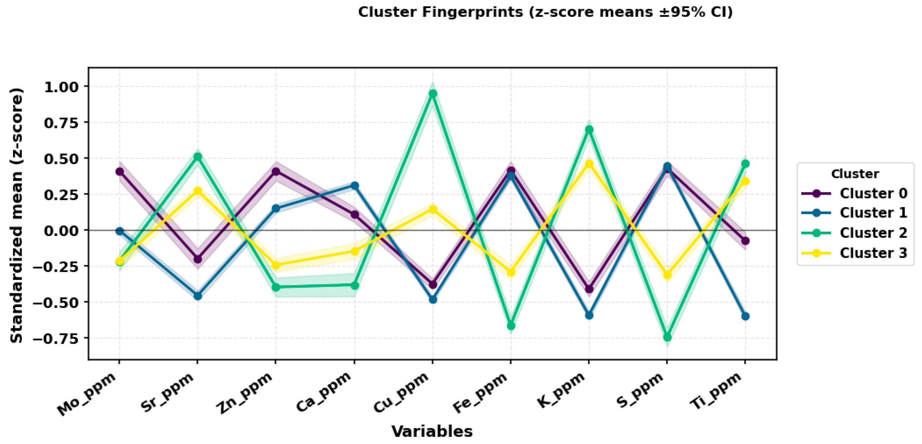
Cluster level geochemical signatures were summarized using fingerprints that plot standardized means and 95 percent confidence intervals across the nine variables (Figure 10). Clear separation is observed for Sr, Zn, Fe, and K, which indicates that these tracers have the strongest discriminating power for the tailings deposit. More moderate offsets on Mo, Ca, S, and Ti reflect gradational behavior that is typical of transitional materials. One zone occupies intermediate values for several elements and therefore acts as a bridge between enriched and depleted regimes. Because values were standardized as deposit wide z scores, the contrasts represent relative enrichment rather than absolute concentrations.

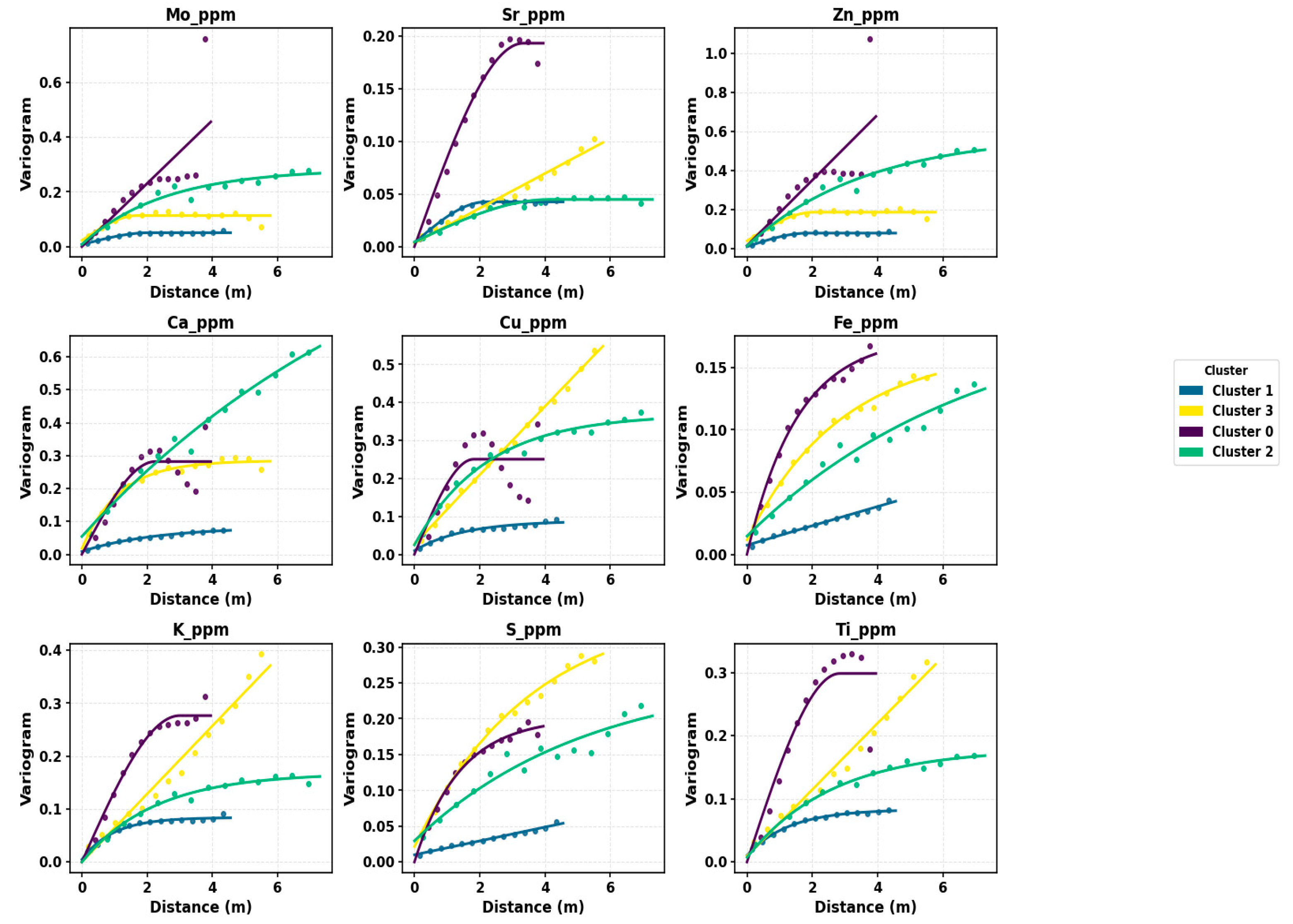
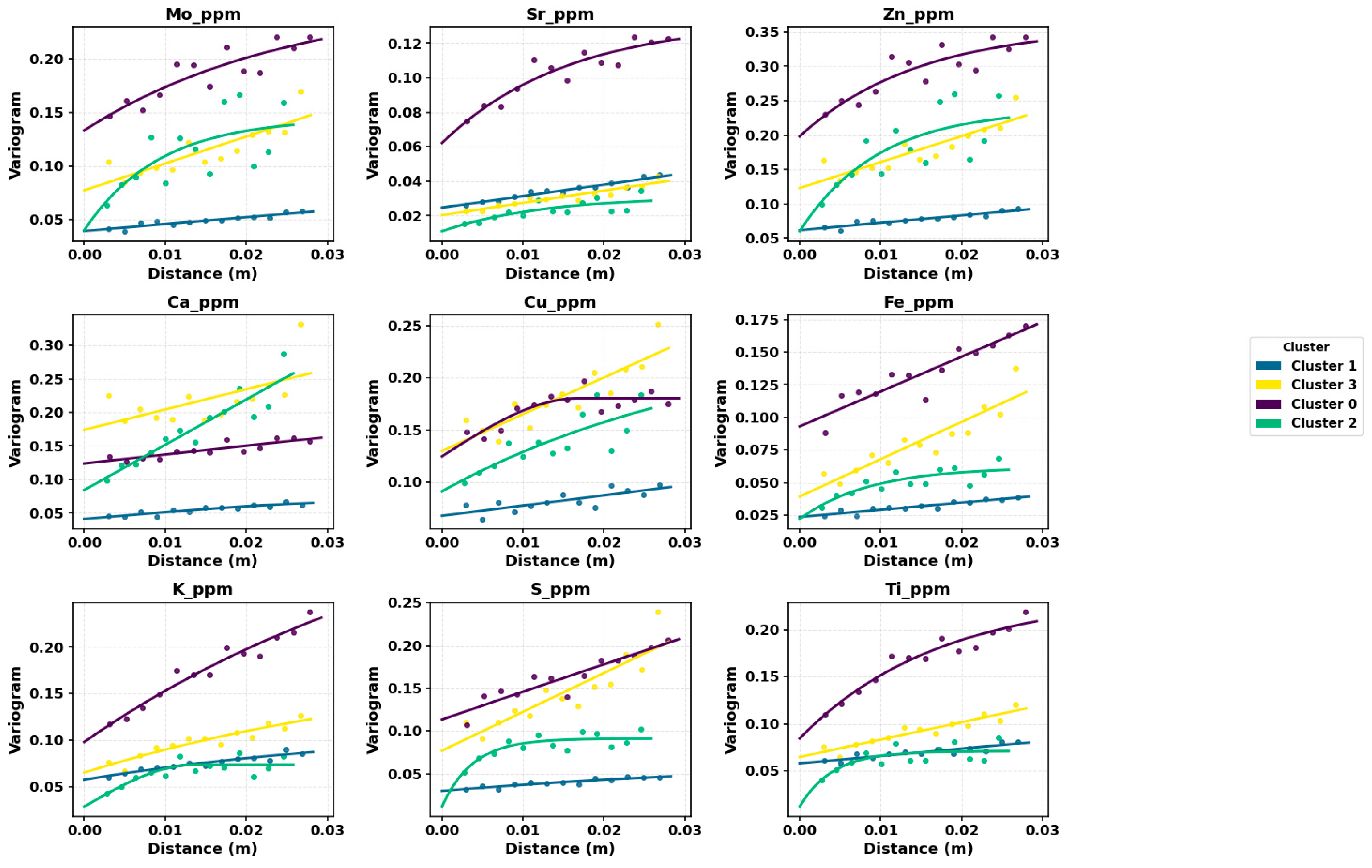
Directional continuity in the GkRNN zones was evaluated with experimental semivariograms computed vertically and horizontally for all nine elements, and spherical models were fitted by least squares (Figure 11 and Figure 12). For the vertical direction, within-hole pairs were formed after ordering samples by depth; for the horizontal direction, plan view pairs were restricted to similar depths using a small vertical tolerance and a search radius set to a fraction of the deposit footprint. Populous zones showed well-defined ranges and modest nuggets in both directions, which indicates strong internal coherence of the GkRNN partitions. In many variables the lateral range exceeded the vertical range, a pattern that matches the bedded architecture expected in a tailings deposit. The clearest structure was observed for Sr, Zn, Fe and K, agreeing with the zone contrasts seen in the variables-versus-depth mosaics and in the cluster fingerprints.

Interpretation in the context of the tailings deposit is therefore straightforward. The large zones appear to represent stratified packages that persist laterally across the footprint, consistent with relatively uniform discharge conditions and settling processes. A rare zone with limited spatial support exhibited short ranges and low sills, which is consistent with patchy or lens-like material produced by local reworking. While uncertainty increases for that zone because pair counts are small, the directional behavior remains compatible with the mapped GkRNN zones.

Taken together, the mosaic level stratification, the alignment of compositional breaks at the scale of individual drillholes, the smooth depthwise proportions, the discriminative fingerprints, and the directionally consistent semivariograms indicate that the workflow captured both composition and structure in a way that is faithful to tailing deposition.

4. Discussion

4.1. Spatial Comparison Between GkRNN, K-Means, and Gaussian Mixture

Spatial coherence and geological plausibility were evaluated by comparing the continuity-aware GkRNN workflow with a conventional k-means baseline and a Gaussian Mixture model. Figure 13 shows the 3D clustering results for the tailings deposit. The GkRNN model produces vertically consistent, sheet-like domains that follow the expected lamination of the tailings body. In contrast, k-means generate highly fragmented patches that oscillate along depth, while the Gaussian Mixture result lies between these two extremes, with somewhat smoother packages than k-means but still more breaks and isolated lenses than GkRNN. These visual differences reflect how each method handles spatial context. GkRNN operates in a spectral space that encodes joint continuity and then regularizes labels along depth with Markov and LSTM sequence models, which encourages persistence where composition and context agree. Both k-means and Gaussian Mixture assign labels point-by-point in feature space and have no built in notion of neighborhood or stratigraphic order, so small geochemical perturbations can flip labels along a borehole.

The limitations of k-means are most evident in drillholes that contain gradual geochemical transitions. Because k-means imposes spherical clusters of similar size in Euclidean space, it tends to break softly varying logs into many small segments and often mistakes local noise for lithological change [46,47]. In drillhole MPT-19-13_AL, for example, the k-means solution splits the log into more than twenty cluster units, which is implausible for laminated tailings with known depositional continuity. The Gaussian Mixture model replaces hard Voronoi partitions with overlapping Gaussian components in the CLR space, which softens some of the abrupt k-means boundaries. Nevertheless, the mixture still treats each depth independently and cannot enforce vertical ordering, so it continues to introduce extra small scale units that do not correspond to distinct depositional campaigns. In contrast, the GkRNN segmentation of the same log remains within a small number of thicker, contiguous packages and places boundaries only where there is clear multielement support. In this sense, the time series character of the downhole data is respected only by GkRNN, which explicitly learns transition patterns along depth, while the other two methods remain purely point-based.

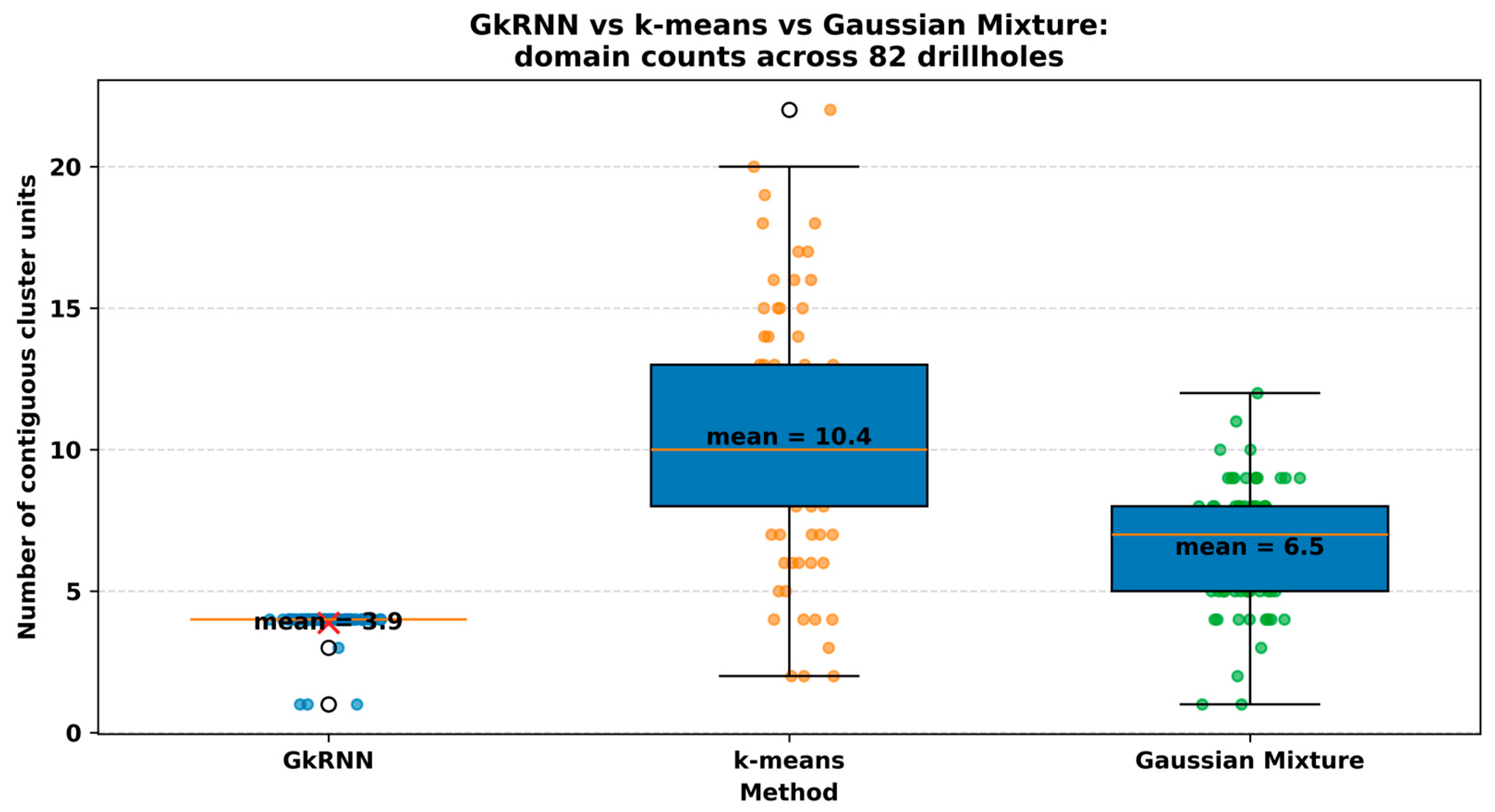
These behavioral differences have direct practical implications. Every additional contiguous unit increases the work required for variogram modeling, grade estimation, and domaining, and propagates noise into block models and short-term planning. Under the contiguous-unit definition used in this study, k-means yields a mean of 10.4 units per drillhole, with a median of 10, a range of 2 to 22, and a standard deviation of 4.2. GkRNN maintains stratigraphic coherence with a mean of 3.85 units per drillhole, a median of 4, a narrow range of 1 to 4, and a standard deviation of 0.59, which reduces the unit count by roughly two-thirds relative to k-means. The Gaussian Mixture model lies between these two, with a mean of 6.5 units per drillhole, a median of 7, a range of 1 to 12, and a standard deviation of about 2.0. Fewer, thicker, and more stable domains from GkRNN translate into simpler and more defensible models, clearer grade-control decisions, and less ambiguity when drawing dig lines, whereas Gaussian Mixture offers only a partial reduction in complexity relative to k-means.

Stability achieved by GkRNN also matches the intended four-layer architecture of the synthetic tailings deposit. Across 82 drillholes, exactly four contiguous units are recovered in 76 holes, corresponding to 93% of the dataset. K-means recovers four units in only four holes (5%), and the Gaussian Mixture model reaches four units in eight holes (10%). The distributions in Figure 14 make this contrast clear. The GkRNN counts form a tight peak centered at four units per hole. Gaussian Mixture shows a broader distribution that is shifted upward but still much closer to the GkRNN peak than to k-means. K-means displays the widest spread and many high-count outliers, which is a classic signature of depthwise label chattering.

Table 1. Global comparison of cluster-unit statistics across 82 drillholes.

Metric	GkRNN	k-means	Gaussian Mixture
Mean units per drillhole	3.85	10.4	6.5
Median	4	10	7
Range	1–4	2–22	1–12
Standard deviation	0.59	4.2	2
Drillholes with exactly 4 units	76/82 (93%)	4/82 (5%)	8/82 (10%)

summarizes these statistics and confirms that GkRNN provides the strongest control on contiguity and realistic thickness, Gaussian Mixture improves over the purely point-based k-means but still allows unnecessary subdivision, and k-means is the least suitable of the three for stratigraphically plausible, planning-ready domaining.

Table 1 summarizes the number of geochemically distinct contiguous units identified per drillhole in the new run. Across 82 drillholes, GkRNN concentrates tightly around four units per hole, with a mean of 3.85, median 4, range 1–4, standard deviation 0.59, and exactly four units in 76 of 82 drillholes (93%). K-means fragments the downhole logs, yielding a mean of 10.4 units per drillhole, median 10, range 2–22, standard deviation 4.2, and only 4 drillholes (5%) with exactly four units. The Gaussian Mixture model provides an intermediate outcome, with a mean of 6.5 units per drillhole, median 7, range 1–12, standard deviation about 2.0, and 8 drillholes (10%) with exactly four units. Together with Figure 13 and Figure 14, these values show that the sequence-regularized GkRNN labeling best preserves stratigraphic coherence and realistic thickness, Gaussian Mixture offers a modest improvement over k-means, and k-means tends to over-segment the logs under the contiguous-unit definition.

4.2. Methodological Contributions of the Continuity-Aware GkRNN Workflow

The continuity-aware GkRNN workflow combines compositional preprocessing, continuity-based similarity, and sequence modeling in a single pipeline. Compositional assays are first mapped with a CLR transformation and a kernel variogram so that the similarity graph reflects both multivariate grade structure and spatial continuity. A spectral embedding of this graph provides a low-dimensional space where clusters are already shaped by spatial dependence, and an elbow analysis in this space selects a small set of clusters that represent the main compositional regimes without chasing local noise. Downhole labels are then treated as depth-ordered sequences: a left-to-right HMM and an LSTM trained on sliding windows promote persistence when composition and context agree and allow changes only when there is multielement support, while a minimum thickness filter removes short, isolated runs. The resulting zones reproduce the depth-ordered mosaics, smooth zone proportions, and compact contiguous unit counts, so compositional breaks and stratigraphic continuity are enforced in a consistent way.

The workflow is built to operate on a regular depth scale. All drillhole assays are composited to a fixed interval before variograms, spectral embedding, and sequence models are fitted, so GkRNN works on equally spaced depth steps and is not tied to any specific physical sampling interval, provided that the chosen support is regular and fine enough relative to vertical correlation ranges and typical facies thicknesses; logs sampled at different intervals or at a new target resolution can be recomposited and the continuity statistics recomputed without changing the architecture. Behavior in the presence of skewed or sparse variables is governed mainly by preprocessing and continuity modeling: after the CLR transform, variables are standardized, joint kernel variogram matrices are regularized by eigenvalue clipping and a small ridge term, and the resulting dissimilarities are rescaled with a median-based parameter τ so that clustering takes place in a fixed low-dimensional spectral embedding that summarizes joint continuity, meaning k-means acts on smoothed, continuity-aware features rather than on raw sparse or heavy-tailed variables. The components of this framework are formulated in a general way and do not rely on features unique to mine wastes, so the same pipeline can, in principle, be applied to fluvial sediments, deep ore bodies, or other geological environments wherever multivariate assays and basic spatial continuity allow joint variograms and sequence statistics to be estimated; tailings are a particularly suitable first test case because dense drilling and stratified, laterally extensive packages from repeated deposition match the continuity-aware facies concept that GkRNN is designed to capture, while other settings would mainly require practical tuning of the variogram lag structure and neighborhood graph to account for channel anisotropy or sparser, deeper drilling.

5. Conclusions

A continuity-aware, sequence-regularized workflow was developed to transform noisy compositional drillhole assays into stratigraphically coherent domains for tailings deposits. The Geostatistical k-means Recurrent Neural Network (GkRNN) integrates centered log-ratio (CLR) preprocessing, a kernel-variogram-based spectral representation, k-means clustering, and depth regularization via a hidden Markov model (HMM) and a long short-term memory (LSTM) network. Applied to 82 drillholes containing nine elements, the method produced a small number of stable zones per hole, smooth depthwise trends, and semivariograms consistent with laminated material. Compared with a conventional k-means baseline and a Gaussian Mixture model, the mean number of contiguous units per hole decreased from 10.4 (k-means) and 6.5 (Gaussian Mixture) to 3.85 with GkRNN, with exactly four units recovered in 93% of holes versus 5% and 10%, greatly simplifying subsequent modeling and planning.

Viewed through the variogram constraints and the HMM, GkRNN can be considered a general clustering approach that promotes spatial continuity and vertical stratigraphic coherence in layered datasets. Because the preprocessing stage is modular, it can be adapted to case-specific applications, which makes the workflow readily extendable to three-dimensional stratigraphic modeling of borehole data beyond tailings. Potential uses include improved constraint of reservoir properties such as porosity and permeability in petroleum settings, as well as characterization of stratiform mineral systems such as Kupferschiefer and of groundwater aquifers.

Future extensions should integrate multi-sensor inputs such as hyperspectral, wireline, and measurement-while-drilling logs, and include uncertainty envelopes around boundaries. Probabilistic recurrent networks and adaptive thickness priors could further refine transitions and capture site-specific depositional patterns. With these enhancements, GkRNN could advance toward near-real-time domaining with explicit quality controls, supporting safer and more efficient tailing re-mining.

References

1. Gitari, M.; Akinyemi, S.; Ramugondo, L.; Matidza, M.; Mhlongo, S. Geochemical fractionation of metals and metalloids in tailings and appraisal of environmental pollution in the abandoned Musina Copper Mine, South Africa. Environ. Geochem. Health 2018, 40, 2421–2439. [Google Scholar] [CrossRef] [PubMed]
2. Zhang, L.; Zheng, L.; Xia, Y.; Qiu, Z. ERT-assisted assessment of geochemical characteristics of tailings profile and environmental risks of heavy metals: A study on a typical sulfide tailings pond. Environ. Earth Sci. 2023, 82, 152. [Google Scholar] [CrossRef]
3. Anvari, K.; Mousavi, A.; Sayadi, A.R.; Sellers, E.; Salmi, E.F. Automatic detection of rock boundaries using a hybrid recurrence quantification analysis and machine learning techniques. Bull. Eng. Geol. Environ. 2022, 81, 398. [Google Scholar] [CrossRef]
4. Silversides, K.L.; Melkumyan, A. Boundary identification and surface updates using MWD. Math. Geosci. 2021, 53, 1047–1071. [Google Scholar] [CrossRef]
5. Soto, F.; Navarro, F.; Díaz, G.; Emery, X.; Parviainen, A.; Egaña, Á. Transitive kriging for modeling tailings deposits: A case study in southwest Finland. J. Clean. Prod. 2022, 374, 133857. [Google Scholar] [CrossRef]
6. Redwan, M.; Rammlmair, D. Understanding Micro-Environment Development in Mine Tailings Using MLA and Image Analysis. In Proceedings of the 10th International Congress for Applied Mineralogy (ICAM); Springer: Berlin/Heidelberg, Germany, 2012; pp. 589–596. [Google Scholar] [CrossRef]
7. Hill, E.J.; Pearce, M.A.; Stromberg, J.M. Improving automated geological logging of drill holes by incorporating multiscale spatial methods. Math. Geosci. 2021, 53, 21–53. [Google Scholar] [CrossRef]
8. Anvari, K.; Benndorf, J. Real Time Mining—A Review of Developments Within the Last Decade. Mining 2025, 5, 38. [Google Scholar] [CrossRef]
9. Benndorf, J. Making use of online production data: Sequential updating of mineral resource models. Math. Geosci. 2015, 47, 547–563. [Google Scholar] [CrossRef]
10. Benndorf, J. Closed Loop Management in Mineral Resource Extraction: Turning Online Geo-Data into Mining Intelligence; Springer Nature: Cham, Switzerland, 2020. [Google Scholar] [CrossRef]
11. Aghahadi, M.H.; Jozanikohan, G.; Asghari, O.; Anvari, K.; Hosseini, S.T. Spatial Clustering of Primary Geochemical Halos Using Unsupervised Machine Learning in Sari Gunay Gold Deposit, Iran. Min. Metall. Explor. 2024, 41, 2741–2760. [Google Scholar] [CrossRef]
12. Caté, A.; Schetselaar, E.; Mercier-Langevin, P.; Ross, P.-S. Classification of lithostratigraphic and alteration units from drillhole lithogeochemical data using machine learning: A case study from the Lalor volcanogenic massive sulphide deposit, Snow Lake, Manitoba, Canada. J. Geochem. Explor. 2018, 188, 216–228. [Google Scholar] [CrossRef]
13. Fouedjio, F.; Arya, E. Locally varying geostatistical machine learning for spatial prediction. Artif. Intell. Geosci. 2024, 5, 100081. [Google Scholar] [CrossRef]
14. Mahmoodi, O.; Smith, R.S.; Tinkham, D.K. Supervised classification of down-hole physical properties measurements using neural network to predict the lithology. J. Appl. Geophys. 2016, 124, 17–26. [Google Scholar] [CrossRef]
15. Horrocks, T.; Holden, E.-J.; Wedge, D. Evaluation of automated lithology classification architectures using highly-sampled wireline logs for coal exploration. Comput. Geosci. 2015, 83, 209–218. [Google Scholar] [CrossRef]
16. Wang, Z.; Li, T.; Zuo, R. Leucogranite mapping via convolutional recurrent neural networks and geochemical survey data in the Himalayan orogen. Geosci. Front. 2024, 15, 101715. [Google Scholar] [CrossRef]
17. Hill, E.J.; Robertson, J.; Uvarova, Y. Multiscale hierarchical domaining and compression of drill hole data. Comput. Geosci. 2015, 79, 47–57. [Google Scholar] [CrossRef]
18. Zaitouny, A.; Small, M.; Hill, J.; Emelyanova, I.; Clennell, M.B. Fast automatic detection of geological boundaries from multivariate log data using recurrence. Comput. Geosci. 2020, 135, 104362. [Google Scholar] [CrossRef]
19. Karimi, A.M.; Sadeghnejad, S.; Rezghi, M. Well-to-well correlation and identifying lithological boundaries by principal component analysis of well-logs. Comput. Geosci. 2021, 157, 104942. [Google Scholar] [CrossRef]
20. Morgan, H.; Elgendy, A.; Said, A.; Hashem, M.; Li, W.; Maharjan, S.; El-Askary, H. Enhanced lithological mapping in arid crystalline regions using explainable AI and multi-spectral remote sensing data. Comput. Geosci. 2024, 193, 105738. [Google Scholar] [CrossRef]
21. Deng, H.; Huang, J.; Liu, Z.; Li, L.; Liu, X.; Wang, X.; Chen, J.; Wu, Z.; Mao, X. Hidden Markov model for spatial analysis of three-dimensional mineralization distribution: Insights into magma flow and mineral exploration targets in the Jinchuan Ni-Cu-(PGE) sulfide deposit, China. Appl. Geochem. 2024, 162, 105911. [Google Scholar] [CrossRef]
22. Ouyang, J.; Zhou, C.; Liu, Z.; Zhang, G. Triangulated irregular network-based probabilistic 3D geological modelling using Markov Chain and Monte Carlo simulation. Eng. Geol. 2023, 320, 107131. [Google Scholar] [CrossRef]
23. Talarico, E.; Leão, W.; Grana, D. Comparison of recursive neural network and Markov chain models in facies inversion. Math. Geosci. 2021, 53, 395–413. [Google Scholar] [CrossRef]
24. Fouedjio, F. A Clustering Approach for Discovering Intrinsic Clusters in Multivariate Geostatistical Data. In Proceedings of the International Conference on Machine Learning and Data Mining in Pattern Recognition; Springer: Cham, Switzerland, 2016; pp. 491–500. [Google Scholar]
25. Fouedjio, F.; Hill, E.J.; Laukamp, C. Geostatistical clustering as an aid for ore body domaining: Case study at the Rocklea Dome channel iron ore deposit, Western Australia. Appl. Earth Sci. 2018, 127, 15–29. [Google Scholar] [CrossRef]
26. Jalloh, A.B.; Kyuro, S.; Jalloh, Y.; Barrie, A.K. Integrating artificial neural networks and geostatistics for optimum 3D geological block modeling in mineral reserve estimation: A case study. Int. J. Min. Sci. Technol. 2016, 26, 581–585. [Google Scholar] [CrossRef]
27. van der Grijp, Y.; Minnitt, R.; Rose, D. Modelling a complex gold deposit with multiple-point statistics. Ore Geol. Rev. 2021, 139, 104427. [Google Scholar] [CrossRef]
28. Anvari, K.; Benndorf, J.; Gerber, G.; Alisch, U. Hybrid geostatistical and deep learning framework for geochemical characterization in historical mine tailings. Sci. Rep. 2025, 15, 35004. [Google Scholar] [CrossRef]
29. Bai, T.; Tahmasebi, P. Accelerating geostatistical modeling using geostatistics-informed machine Learning. Comput. Geosci. 2021, 146, 104663. [Google Scholar] [CrossRef]
30. Frascoli, F.; Hudson-Edwards, K.A. Geochemistry, mineralogy and microbiology of molybdenum in mining-affected environments. Minerals 2018, 8, 42. [Google Scholar] [CrossRef]
31. Alicja, K.; Grzegorz, C. Strontium leaching from municipal waste subjected to incineration. Environ. Geochem. Health 2024, 46, 220. [Google Scholar] [CrossRef]
32. Dart, R.C.; Wittwer, P.D.; Barovich, K.M.; Chittleborough, D.; Hill, S. Strontium isotopes as an indicator of the source of calcium for regolith carbonates. In Proceedings of the Regolith; CRC LEME: Bentley, WA, Australia, 2004; pp. 67–70. [Google Scholar]
33. Hayes, S.M.; Root, R.A.; Perdrial, N.; Maier, R.M.; Chorover, J. Surficial weathering of iron sulfide mine tailings under semi-arid climate. Geochim. Cosmochim. Acta 2014, 141, 240–257. [Google Scholar] [CrossRef] [PubMed]
34. Murray, J.; Kirschbaum, A.; Dold, B.; Mendes Guimaraes, E.; Pannunzio Miner, E. Jarosite versus soluble iron-sulfate formation and their role in acid mine drainage formation at the Pan de Azúcar mine tailings (Zn-Pb-Ag), NW Argentina. Minerals 2014, 4, 477–502. [Google Scholar] [CrossRef]
35. Lindsay, M.B.; Moncur, M.C.; Bain, J.G.; Jambor, J.L.; Ptacek, C.J.; Blowes, D.W. Geochemical and mineralogical aspects of sulfide mine tailings. Appl. Geochem. 2015, 57, 157–177. [Google Scholar] [CrossRef]
36. Aitchison, J. The statistical analysis of compositional data. J. R. Stat. Soc. Ser. B (Methodol.) 1982, 44, 139–160. [Google Scholar] [CrossRef]
37. Pawlowsky-Glahn, V.; Buccianti, A. Compositional Data Analysis: Theory and Applications; John Wiley & Sons: Chichester, UK, 2011. [Google Scholar]
38. Fouedjio, F. A spectral clustering method for large-scale geostatistical datasets. In Proceedings of the Machine Learning and Data Mining in Pattern Recognition: 13th International Conference, MLDM 2017, New York, NY, USA, 15–20 July 2017; pp. 248–261. [Google Scholar]
39. Wackernagel, H. Multivariate Geostatistics: An Introduction with Applications; Springer Science & Business Media: Berlin/Heidelberg, Germany, 2003. [Google Scholar]
40. Rossi, R.E.; Mulla, D.J.; Journel, A.G.; Franz, E.H. Geostatistical tools for modeling and interpreting ecological spatial dependence. Ecol. Monogr. 1992, 62, 277–314. [Google Scholar] [CrossRef]
41. Jain, A.K. Data clustering: 50 years beyond K-means. Pattern Recognit. Lett. 2010, 31, 651–666. [Google Scholar] [CrossRef]
42. MacQueen, J. Some Methods for Classification and Analysis of Multivariate Observations. In Proceedings of 5-th Berkeley Symposium on Mathematical Statistics and Probability; University of California Press: Berkeley, CA, USA, 1967. [Google Scholar]
43. Bishop, C.M.; Nasrabadi, N.M. Pattern Recognition and Machine Learning; Springer: Berlin/Heidelberg, Germany, 2006; Volume 4. [Google Scholar]
44. Davis, J.C.; Sampson, R.J. Statistics and Data Analysis in Geology; Wiley: New York, NY, USA, 1986; Volume 646. [Google Scholar]
45. Elman, J.L. Finding structure in time. Cogn. Sci. 1990, 14, 179–211. [Google Scholar] [CrossRef]
46. Anvari, K.; Mousavi, A.; Sayadi, A.R.; Afzal, P.; Sellers, E.; Salmi, E.F. A Hybrid Recurrence Analysis and Wavelet Transformation for Rock Boundary Identification. Preprint 2024. Available online: https://doi.org/10.2139/ssrn.5049654 (accessed on 20 March 2024).
47. Zaitouny, A.; Ramanaidou, E.; Hill, J.; Walker, D.M.; Small, M. Objective domain boundaries detection in new Caledonian nickel laterite from spectra using quadrant scan. Minerals 2021, 12, 49. [Google Scholar] [CrossRef]
Figure 1. Pair plot of multivariate geochemical variables.
Minerals 15 01249 g001
Figure 2. Geological maps of the tailings deposit. (a) Plan view geological map; (b) longitudinal section along structural trend.
Minerals 15 01249 g002
Figure 3. Comparison of skewness and kurtosis for the original and CLR-transformed geochemical data.
Minerals 15 01249 g003
Figure 4. Overview of the GkRNN Workflow.
Minerals 15 01249 g004
Figure 5. Elbow plot of within-cluster inertia computed in the spectral space Z spec for k = 2–8. The dashed vertical line marks the selected elbow at k = 4.
Minerals 15 01249 g005
Figure 6. Variables versus depth across all boreholes, colored by GkRNN zones.
Minerals 15 01249 g006
Figure 7. Elemental depth profiles with cluster assignments (MPT-19-01_AL).
Minerals 15 01249 g007
Figure 8. Zone proportions versus depth for the tailing deposit. Stacked ribbons were computed in 0.5 m bins; colors correspond to the final GkRNN zones; depth increases downward.
Minerals 15 01249 g008
Figure 9. Three-dimensional facies model illustrating vertical and lateral variations within the borehole footprint. Colors indicate the final GkRNN zones.
Minerals 15 01249 g009
Figure 10. Cluster fingerprints across nine variables showing mean z scores with ±1.96 SEM.
Minerals 15 01249 g010
Figure 11. Vertical variograms by zone (experimental points; fitted models).
Minerals 15 01249 g011
Figure 12. Horizontal variograms by zone (experimental points; fitted models).
Minerals 15 01249 g012
Figure 13. Three-dimensional geological visualization of clustered facies generated using (top) the continuity-aware GkRNN workflow, (middle) k-means clustering, and (bottom) Gaussian Mixture models. Each plot shows drillhole trajectories colored by the assigned cluster labels, with depth plotted along the vertical axis.
Minerals 15 01249 g013
Figure 14. Boxplot comparing the number of contiguous cluster units per drillhole for GkRNN, k-means, and Gaussian Mixture.
Minerals 15 01249 g014